Acoustic angiography: a new imaging platform for high resolution mapping of microvasculature and tumor assessment
Ryan C. Gessner
A dissertation submitted to the faculty of the University of North Carolina at Chapel Hill in partial fulfillment of the requirements for the degree of Doctor of Philosophy in the Department of Biomedical Engineering.
Chapel Hill 2013
Approved by:
Paul A. Dayton, Ph.D. Stephen R. Aylward, Ph.D. Caterina M. Gallippi, Ph.D. David Lalush, Ph.D.
c
ABSTRACT
RYAN C. GESSNER: Acoustic angiography: a new imaging platform for high resolution mapping of microvasculature and tumor assessment.
(Under the direction of Paul A. Dayton, Ph.D.)
Statistically, one in four Americans will die from cancer. Many new tumor detection and therapeutic approaches have improved patient outcomes, but cancer continues to run rampant in our country; it claimed the lives of 1.6 million Americans in 2012. To put this number of annual deaths in perspective, it is over 500 times the number of people who died in the horrific attacks on September 11, 2001. This dissertation does not offer either an antidote to the disease, nor a detection mechanism appropriate for all tumor types. It does, however, present the description and characterization of a novel dual-frequency ultrasound imaging transducer, capable of operating in a new imaging mode we call ‘acoustic angiography.’ These images offer high resolution and high contrast 3D depictions of the microvasculature; herein we demonstrate its cancer assessment utility by way of multiple imaging studies.
the imaging approach, acoustic angiography, enabled by our new dual-frequency ultra-sound transducer, could eventually be used to detect and monitor tumors in a clinical imaging context.
This dissertation supports the following three hypotheses:
1. A prototype dual-frequency ultrasound transducer can be used to de-pict in vivo microvasculature,
2. These microvascular images can be quantitatively assessed as a means to characterize the presence of a tumor, and evaluate tumor response to therapy, and
To my teachers and mentors, who for my entire life have entertained a daily barrage of but-what-if-THIS-happened?! questions. By doing so they have each nurtured my
curiosity about the underlying mechanics of that mysterious beast: nature. Without them, the questions driving the research within this dissertation might never
ACKNOWLEDGMENTS
I would like to acknowledge my family for their unyielding support throughout the last 27 years of my life. I also could not have asked for a better graduate school advisor than Paul Dayton. Liz Bullitt’s work in the quantitative analysis of vessel morphologies, combined with her willingness to mentor me (essentially only moments
TABLE OF CONTENTS
Table of Contents . . . vii
List of Figures . . . xi
List of Tables . . . xiv
1 Introduction . . . 1
1.1 Cancer imaging with ultrasound . . . 1
1.2 Contrast ultrasound . . . 3
1.3 Dissertation scope and objectives . . . 6
2 Detecting cancer’s vascular footprint . . . 8
2.1 Detecting cancer’s footprint . . . 8
2.1.1 Pathologic tissue’s aberrant vessel morphologies . . . 9
2.1.2 How are vessels extracted from images? . . . 12
2.1.3 How are vessel structures quantified? . . . 15
2.2 Detecting molecular signatures of disease . . . 17
2.2.1 Ultrasonic molecular imaging . . . 19
2.2.2 Challenges in molecular imaging with ultrasound . . . 22
3 Acoustic angiography - a new contrast imaging approach . . . 25
3.1.1 Materials and methods . . . 27
3.1.2 Results . . . 35
3.1.3 Discussion . . . 44
3.1.4 Conclusion . . . 49
3.2 High resolution assessment of vessel architecture - ex vivo tissue samples 49 3.2.1 Materials and methods: . . . 53
3.2.2 Results . . . 59
3.2.3 Discussion and concluding remarks . . . 66
3.3 Acoustic angiography for assessing microvasculature structure: pilot in vivo studies . . . 72
3.3.1 Animal imaging . . . 72
3.3.2 Results . . . 74
3.3.3 Discussion and summary . . . 81
4 Toward the detection of aberrant vessel morphologies with acoustic angiography . . . 83
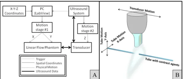
4.1 3D microvessel-mimicking ultrasound phantoms produced with a scan-ning motion system . . . 83
4.1.1 Materials and methods . . . 85
4.1.2 Results . . . 88
4.1.3 Discussion and conclusions . . . 91
4.2 Quantifying vessel structure in controlled in vitro context . . . 94
4.2.1 Methods . . . 94
4.2.2 Results . . . 98
4.2.3 Conclusions and proposed future work . . . 100
5.1 Detecting aberrant vessel morphologies with acoustic angiography . . . 102
5.1.1 Materials and methods . . . 103
5.1.2 Results . . . 108
5.1.3 Discussion . . . 117
5.2 Assessing tumor therapeutic response with acoustic angiography . . . . 119
5.2.1 Methods . . . 121
5.2.2 Tumor model . . . 121
5.2.3 Results and discussion . . . 127
5.2.4 Concluding remarks . . . 138
6 Radiation force enhanced molecular imaging . . . 141
6.1 Molecular imaging with the dual-frequency prototype . . . 143
6.1.1 Methods . . . 143
6.1.2 Results . . . 145
6.1.3 Discussion . . . 148
6.1.4 Concluding remarks . . . 149
6.2 Volumetric molecular imaging with a clinical system . . . 150
6.2.1 Materials and methods . . . 150
6.2.2 Results . . . 158
6.2.3 Discussion . . . 164
6.2.4 Conclusion . . . 169
7 Closing remarks . . . 170
7.1 The future acoustic angiography . . . 171
7.2 The future molecular imaging with ultrasound . . . 172
A Microbubble contrast agent formulation . . . 174
A.2 In vitro targeted agents . . . 174
A.3 In vivo targeted agents . . . 174
B IEEE December 2010 Cover Image . . . 176
C Ex vivo liver scaffold preparation . . . 178
LIST OF FIGURES
1.1 Dayton lab ultrasound equipment . . . 2
1.2 Overview of microbubbles . . . 3
1.3 Overview of contrast imaging approaches . . . 5
2.1 Intravital microscopy image of vasculature . . . 11
2.2 Quantifying vessel morphologies . . . 16
2.3 Qualitative illustration of the effect of resolution on vessel imaging . . . 18
2.4 Cartoon illustration of molecular imaging with ultrasound . . . 20
2.5 Schematic of targeted contrast accumulation over time . . . 21
2.6 Cartoon illustration of radiation force enhanced targeting . . . 23
3.1 Dual-frequency probe schematic . . . 28
3.2 Dual-frequency probe beam maps . . . 36
3.3 Dual-frequency probe axial pressure maps . . . 37
3.4 Time domain responses from contrast and tissue . . . 37
3.5 Frequency domain responses from contrast and tissue . . . 38
3.6 Contrast to tissue ratios computed with dual-frequency probe . . . 39
3.7 Example acoustic angiography images of contrast in rat kidney . . . 40
3.8 Comparision of all imaging modes tested . . . 42
3.9 Comparision of imaging proficiency with respiratory gating . . . 43
3.11 Overview of bioeffect-inducing acoustic parameters . . . 45
3.12 Liver scaffold imaging chamber . . . 54
3.13 Schematic of image pipeline . . . 62
3.14 Biomatrix perfusion stability data . . . 63
3.15 All image data acquired of biomatrix samples . . . 64
3.16 Quantitative comparision between samples of biomatrix vascularity . . 65
3.17 3D renderings of the three liver scaffolds . . . 67
3.18 Overlay of contrast and b-mode . . . 75
3.19 Comparison of tumor-bearing and healthy tissue . . . 77
3.20 Comparison of Acoustic Angiography with photoacoustics . . . 79
3.21 Overlay of contrast and b-mode . . . 80
4.1 3D vessel phantom schematic . . . 86
4.2 3D vessel phantom generation cartoon . . . 87
4.3 Generating phantoms with increasing tortuosity . . . 89
4.4 Creating a bifurcating vessel network . . . 90
4.5 Measuring contrast sensitivity vs. depth . . . 91
4.6 Vessel phantoms used for segmentation . . . 95
4.7 Example segmentations . . . 96
4.8 Quantifying error in vessel phantom segmentations . . . 99
5.1 Microvasculature comparison between Control and Tumor-bearing tissue volumes . . . 110
5.2 Example vessel centerlines . . . 111
5.3 Quantitative comparisons between tumor and control vessels . . . 115
5.4 Retrospective subsampling p values . . . 116
5.6 Treatment room for irradiations . . . 123
5.7 Treatment timeline . . . 124
5.8 Elliptical ROI Computation . . . 126
5.9 Pretreatment tumor volumes . . . 127
5.10 Post-treatment survival curves . . . 128
5.11 Post-treatment animal weights . . . 129
5.12 Radiation beam simulation . . . 131
5.13 Tumor growth: All groups . . . 132
5.14 Tumor growth: 20 Gy group . . . 133
5.15 Perfusion of tumors post therapy . . . 134
5.16 Perfusion volume ratios post therapy . . . 135
5.17 Power analysis . . . 137
6.1 Cartoon schematic of RF application . . . 144
6.2 Acoustic and optical detection of successful RF . . . 146
6.3 3D targeting results . . . 147
6.4 Visualizing targeting signal . . . 148
6.5 Radiation force in vitro schematic . . . 153
6.6 Radiation force in vitro push optimization results . . . 159
6.7 Results from the cummulative error function analysis . . . 160
6.8 Effects of radiation force on microbubble targeting in vivo . . . 161
6.9 3D rendering of microbubble targeting in vivo . . . 163
C.1 Decellularization process . . . 179
LIST OF TABLES
3.1 Imaging pressures tested . . . 32
3.2 Blood flow rates tested . . . 34
4.1 Summary of segmentation consistency results . . . 98
5.1 Summary of tortuosity metrics . . . 112
5.2 Summary of statistical tests - tortuosity . . . 113
5.3 Summary of recent preclinical ultrasound imaging studies . . . 121
CHAPTER 1 INTRODUCTION
1.1 Cancer imaging with ultrasound
This dissertation is devoted to presenting and discussing work surrounding the devel-opment of ultrasound imaging tools to improve cancer research and diagnostics. It is well established that a tumor’s growth is highly dependent on its blood supply, which is under constant and chaotic remodeling as a neoplasm evolves. [1] Thus, there exists a widespread demand within the clinical and preclinical cancer research communities for methods to noninvasively and quantitatively assess tumor vascularization and blood supply. These research communities constantly seek to improve their imaging meth-ods to thereby increase their understanding of tumor progression, and the quality of their diagnostic and therapeutic decision making. Ultrasound offers several advantages over other imaging modalities for the preclinical and clincial assessment of tumors and tumor blood flow.
Widespread accessability
inexpensive, costing only a fraction of what other modalities’ systems cost (magnetic resonance (MR) and x-ray computed tomography(CT)). This makes ultrasound much more accessible to rural or less affluent communities, and much more financially viable for longitudinal studies with many timepoints, or drug efficacy studies with many sub-jects. Using other imaging approaches, these large-cohort or multiple-timepoint studies could be prohibitively expensive.
Noninvasive and real time
Ultrasound images do not require ionizing radiation to create images, as is the case with x-ray CT. Whereas longitudinal studies with CT imaging necessitate careful dose con-siderations, longitudinal ultrasound acquisitions are not problematic, enabling physi-cians or preclinical researchers to assess changes in tumor size and blood perfusion at many timepoints before, and throughout treatment. Images are also real-time, enabling rapid feedback for imaging transducer position to optimize image quality.
1.2 Contrast ultrasound
Because the cost of drug development is so high - many estimates put drug develop-ment, from initial compound screening through clinical trials at over 1 billion USD [2] - preclinical drug researchers continually seek to drive down costs of their studies. Some of these preclinical drug researchers have started using high resolution ultrasound to evaluate their candidate therapeutics.[3; 4; 5; 6]. Lipid-encapsulated microbubbles are often implemented as contrast agents during these ultrasound studies to improve detection of blood flow [7]. Microbubbles typically consist of a high molecular weight gas core stabilized with a lipid. High molecular weight gasses are preferred due to their low solubility in blood and poor diffusivity through their encapsulating shell. This extends microbubble circulation timein vivo. The acoustic impedance mismatch between the gas cores of microbubbles and the surrounding blood and tissue is ap-proximately four orders of magnitude [8], causing them to scatter significantly more ultrasound energy than blood components, and thus enabling improved sensitivity of ultrasound to blood flow (Figure 1.2). Their use requires an intravascular injection of a solution of microbubbles immediately before an imaging exam. After their injection, the microbubble contrast agents traverse the circulatory system with similar rheology to erythrocytes [9].
The most basic method of contrast enhanced ultrasound relies on receiving the acoustic signal scattered from microbubbles at the fundamental imaging frequency. One limitation to this detection method is that echoes from both tissue and microbub-bles are in the same frequency band. This necessitates a large quantity of injected microbubbles to compete with the inherent and unwanted tissue backscatter. However, owing to the broadband and nonlinear acoustic responses of these gas-filled spheres it is possible to overcome this limitation with other detection strategies. The most powerful microbubble imaging methods are derived from the nonlinear responses of mi-crobubbles to ultrasound, providing distinct differences in microbubble echo signatures when compared with the linear responses of tissue and blood. Imaging modes such as harmonic imaging [10], subharmonic imaging [11; 12], phase inversion [13; 14], contrast pulse sequence (CPS) imaging [15; 16], and harmonic contrast imaging [17] exploit mi-crobubbles’ nonlinear response; all of these methods provide improved contrast-to-tissue ratios compared with the previously described fundamental mode imaging. Figure 1.3 provides a cartoon overview behind the pulsing schemes used to create images from the nonlinear oscillations of contrast agents in response to ultrasound pulses. Although these nonlinear imaging methods are now widely utilized in commercial ultrasound sys-tems operating in the 1 to 15 MHz range, they are more challenging to implement in high-frequency ultrasound systems. One reason for this is that optimal microbubble response requires excitation near the resonant frequency [18], which is approximately 14 to 1.5 MHz for lipid-encapsulated bubbles that are 0.8 to 4µm in diameter, respec-tively. Most commonly available commercially produced microbubbles fall within this diameter range.
Figure 1.3: A cartoon illustration of how CPS and acoustic angiography are distinct from fundamental mode imaging. The ‘Resulting echoes’ column illustrates the non-linear responses of microbubbles to different polarities and frequencies of pulses. HPF: ‘high pass filter.’
model (mouse or rat) requires higher resolution than most clinical systems will al-low. This mismatch between microbubble resonance frequency and preclinical system imaging frequency provided the motivation behind the creation of a novel ultrasound imaging transducer capable of circumventing this tradeoff. This transducer is addressed in Chapter 3.1.
vessel network structure as a means to understand disease progression [32; 33; 29; 34]. Of particular interest is vessel tortuosity, or bendiness which is a morphological abnormality exhibited by cancerous vasculature in both humans and rodents [35; 36], and has been used as a marker for disease state and therapeutic response in clinical studies based on image-derived data [37; 38]. This effect will be described in more detail in Chapter 2.
Because the US Food and Drug Administration (FDA) has practiced excessive cau-tion with respect to microbubble contrast agents, there is currently only one approved clinical application which implements a contrast ultrasound imaging protocol. Their use in other applications such as liver, kidney, thyroid, prostate, and breast tumor as-sessment, is becoming increasingly widespread, however, in several European and Asian countries. Additionally, as described above, there are a host of exciting new applica-tions being developed in the preclinical realm with potential for clinical translation. Over the next decade, it is likely that the US clinical community will begin catching up with their European and Asian colleagues with respect to the frequency with which they implement these powerful contrast ultrasound imaging approaches. This thesis is primarily devoted to the research and results surrounding one of these new contrast imaging approaches, acoustic angiography. This imaging technique, while maybe years away from actual clinical use, is an exciting advance in the field.
1.3 Dissertation scope and objectives
CHAPTER 2
DETECTING CANCER’S VASCULAR FOOTPRINT
The first section of this chapter introduces the effect of cancer-associated vasculature having abnormal morphologies, and how these distinct features are detectable by a quantitative algorithm (Chapter 2.1). The second section describes another method of detecting cancer with ultrasound contrast agents, called ‘molecular imaging.’ (Chapter 2.2)
2.1 Detecting cancer’s footprint
Tumor growth beyond 2 mm3 has been shown to depend on angiogenesis, which is defined as the formation and recruitment of new microvessels from existing vessels. [39; 40; 41]. There are many differences between vessels associated with angiogenic tumors and healthy vessels which can be used as diagnostic indicators of tumor pres-ence and malignacy. For this dissertation, the scope of tumor assessment by way of aniogenisis detection is confined to two facets of vascular composition: (1) vascular
Note: This chapter has two sections, both of which draw from previous published material. Pre-viously published material was reprinted with permission from the publishers.
Chapter 2.1: Ryan C. Gessner, Stephen Aylward, Paul A. Dayton, Imaging tortuosity: the po-tential utility of acoustic angiography in cancer detection and tumor assessment. Imaging in Medicine, 4(6):581-583, 2012. editorial
architecture (both at the individual vessel level, and at the network level) and (2) an-giogenic molecular markers expressed on the vascular endothelium. The following two sections describe these vascular features in greater detail, and provide some background information on detection strategies.
2.1.1 Pathologic tissue’s aberrant vessel morphologies
The morphology and structure of the vasculature associated with malignant tumors has long been observed to be chaotic and unusual compared with that of healthy tissues. In tumors, vessel diameters and branching patterns appear random, and the actual trajectories charted through the 3D tumor volume are often tortuous [36; 42]. These morphological abnormalities are hypothesized to be a result of a number of compli-cated physiological effects occurring in parallel, such as tumor cells’ high metabolic demand and their unusual microenvironment (hypoxic, acidic and so on). These fac-tors contribute to a heightened level of angiogenic activity in and around the tumor, which becomes a self-amplifying cycle when the newly formed vessels fail to supply the tumor cells’ insatiable appetite for nutrients [43]. The heightened angiogenic activ-ity also causes the basement membrane and support structure of the vessels to break down. Additionally, the poor organization of the vessel network results in an increase in pressure within the vessels, which is further exacerbated by the absence of lymphatic drainage from the tumor stroma.
tissue. Second, a segmentation approach must be able to extract vessels from the image volumes in a repeatable and reliable way. This stage usually requires some user input and feedback, although automated approaches allow for higher throughput and thus would be more amenable to clinical implementation. Finally, a classification algorithm based on the segmented vessel data that indicates the presence or degree of pathology is needed. Morphological features can be examined at either the vessel level (e.g., the tortuosity of a single vessel) or at the network level (e.g., the fractal dimension of the vessel tree). Indirect observations of cancer-associated vascular abnormalities are far more prevalent in the clinic today. Examples include measures of overall tissue per-fusion and vessel permeability. These types of measurements are powerful indications of tumor presence and malignancy, but they are limited to more global estimations of vessel morphology within a tissue volume, and thus are insensitive to subtle changes oc-curring therein. These two types of observations (direct and indirect) have been shown to provide independently useful diagnostic information [44]. It is, therefore, unlikely that direct assessments of vascular structure will ever replace existing cancer imaging approaches; however, rather they will compliment them with additional diagnostically powerful information. This could result in a hybrid cancer-assessment approach that is more sensitive than either component alone.
Diagnostic information gleaned from vascular architecture
Figure 2.1: Comparison of cancerous vasculature viewed at different scales by differ-ent imaging modalities. Top: Intravital microscopy images from the Dewhirst lab at Duke University of tumor cells growing within a window chamber model in a rat (scale bar = 200 µm). The images illustrate vascular morphological abnormalities occurring within days of implantation of cancer cells. (Figure portions, from [35], reprinted with permission). Bottom: a maximum intensity projection through an acoustic angiogra-phy dataset illustrating the same type of morphological abnormalities both within and surrounding the tumor margins (dashed yellow line).
study of patients with intracranial neoplasms,[44] and the two methods were shown to provide independently useful diagnostic information. The renormalization of tumor vasculature is also of great interest to researchers and clinicians alike, as anticancer therapies, when effectively quelling a tumor’s progression, have been shown to have a rapid effect on the local vascular morphology. This normalization of vessels has served as an indication of eventual tumor volume reduction and the lack of normalization has correspondingly been associated with poor therapeutic response [48].
Thus the motivation for applying a quantitative vessel-morphological analysis to preclinical models of cancer is apparent, as most anti-cancer drug studies are performed in small rodents. To date, most recent progress in ultrasound assessment of therapeutic response has been in molecular and perfusion imaging, and there are some groups who have used 3D high frequency Doppler techniques to image vascular networks. Analyses of vessel network and vessel morphologies based on segmentations from ultrasound data, however, are scarce, though they have been achieved at lower imaging frequencies (and thus lower spatial resolution) in human thyroid and breast tumors imaging studies. [32; 33; 29; 34; 49] Analyzing the morphology of a vascular network within a diseased tissue volume provides a very sensitive method to assess the effects of therapy, which is particularly necessary when clinicians are seeking to tune their personalized therapeutic approaches [50].
2.1.2 How are vessels extracted from images?
The following is an overview of how the segmentation algorithm used throughout this project functions. The mechanics of the algorithm are discussed at length in [51].
Finding the vessel’s centerline:
vessel selected. The gradient of the image is followed at the location the user specified until a local intensity maximum is reached (assumed to be the true center of the vessel).
Following the vessel’s centerline:
Once an intensity ridge has been found, the extractor looks for what direction the vessel is traveling. This information is gleaned from the Hessian matrix, which allows the extractor to find the direction of least curvature, important in this case as this direction will be the one along an intensity ridge (i.e. normal to the plane bisecting the vessel, and in the direction of the vessel’s trajectory). The next point along the vessel’s centerline is then determined by stepping the normal plane at the intensity ridge a very small distance in the previously described direction of least curvature. The assumption here is that if the centerline is representing an anatomically relevant tube (vessel), its smooth trajectory will necessitate it passing through that shifted plane. The next intensity ridge is then found at the location of the shifted normal plane, and a new vessel trajectory and normal plane determined at this new intensity ridge. This process is repeated iteratively in both positive and negative directions from its initial starting point.
Determining vessel radius
direction, the r that will result in the most stable configuration is when r = R. The ex-tractor tests scales for vessel radius which are within 10% of the previous measurement of vessel radius, which assumes that the radius of anatomically relevant tubes will not rapidly fluctuate (an often accurate assumption, especially since the step size between centerline points is less than one voxel, so if the radius is increasing by more than 10% within that small distance, it’s probable that the tube being extracted is not actually a vessel).
When does the extractor know to stop?
There are several criteria which result in the termination of a vessel extraction. These are tested at each point along the extraction. If a ridge does not exist in the shifted normal plane, the extraction will terminate (this could occur if the intensity drops below the noise level, as would be the case when large vessels feed sub-resolution capillary beds). Additionally, if a junction is encountered, the extraction will terminate. A T-junction would result in the vessel trajectory at the next test point along the centerline not falling within a specified “cone of acceptability.”
Finally, there are several conditions that must be satisfied for a test location to be deemed a ‘ridge point,’ or valid location for a vessel centerline coordinate. These are listed as follows:
1. It must be on a convex intensity ridge. Mathematically this can be verified by ensuring the eigenvalues of the Hessian matrix at this location are negative.
2. It must be a local intensity maximum. Mathematically this can be demonstrated if the projections of the gradient at this location are equal to zero.
more elliptical in cross-section.
2.1.3 How are vessel structures quantified?
After an ensemble of microvessel centerlines had been extracted, their morphologies were quantified via previously established metrics for tortuosity [52]. These metrics, which provide a means to assess two distinct types of centerline tortuosity, were the distance metric (DM) and sum of angles metric (SOAM). The DM is a measure of how far a curve meanders between its end points and is computed as the ratio of the length of the extracted vessel path and the length of the secant line between the vessel’s start and end. The SOAM is an index of vessel tortuosity that is computed by integrating the angular changes occurring between successive pairs of points along the vessel’s centerline, normalized by the total vessel path length. (Figure 2.2)
Relationship between imaging system resolution and tortuosity metrics Assuming the same vessel is imaged by two distinct imaging systems, its digitized rep-resentation also will be different and thus the reported tortuosity values for that vessel’s two image-derived segmentations could be reported as different. What follows is a short overview on the relationship between the imaging system’s acquisition characteristics, and the reported tortuosity for a vessel imaged by that system.
Figure 2.2: A cartoon illustration of how the DM and SOAM are computed from the vessel centerlines.
and is imaged by a system with isotropic resolution in the x and y axes of distance R. The data is discretized by pixels of widthp for display. There are multiple scenarios in which the imaging system parameters (R and p) could bias tortuosity measurements computed from the segmentationS(x,y) for continuous curve C(x,y).
inflate the tortuosity values reported for a vessel. In the presence of this type of p>R
quantization error, the SOAM values will be significantly more affected, since part of its computation involves the integral of these angular deviations between successive points. (Figure 2.2) The DM will also be impacted by this type of error, since the ping-ponging centerline of S(x,y) has a longer path length than the smooth centerline
C(x,y), with the same secant cord between the end points, though to less of a degree, since the path length errors away from the true centerline to not contribute appreciably to the overall path length, especially for anatomically relevant curves.
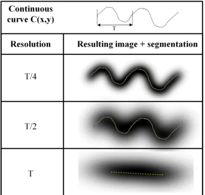
Another way the imaging system can bias the results of the tortuosity computation is if the resolution, R, is too close in size to the spatial period of the vessel being imaged (assume p<R and quantization errors are no longer significant). One should think of this in terms of the Nyquist-Shannon sampling theorem. The Nyquist-Shannon criterion states that for a continuous periodic curve to be accurately defined by a discretized representation, a sampling frequency of at least twice the frequency of the periodic signal must be implemented. Equivalently, in spatial units this means that the resolution of the imaging system must be at most half of the period of the curve
C(x,y). If the condition (R ≤ T
2) does not hold, then the curve will be aliased (Figure
2.3). Practically speaking, this means for an imaging system with R = 150 µm, the smallest periodic deviation which could be reliably imaged has a period of 300 µm. This relationship is more quantitatively established in Chapter 4.
2.2 Detecting molecular signatures of disease
Figure 2.3: A simulation of a continuous vessel curve, C(x,y), being sampled by an imaging system at three different resolutions: T/4, T/2, and T, whereT is the spatial period of the main spatial frequency in C(x,y). Simulated segmentations, S(x,y) are overlaid in yellow.
in vivo in which the radiation force pushing and the imaging are achieved on the same clinical ultrasound system.
2.2.1 Ultrasonic molecular imaging
Molecular imaging with ultrasound is typically performed as follows: an ultrasound transducer is fixed in position over the region of interest with a mechanical arm to avoid motion artifacts from operator movement. A targeted contrast agent is administered into the peripheral vasculature, often through a tail vein during serial imaging studies in rodents. Prior to imaging, a waiting period of approximately 4-30 minutes is required, depending on contrast agent circulation characteristics.[54] During this period, there is a first phase when the targeted contrast agents accumulate in the microvasculature, followed by a second phase when freely circulating agents are cleared from the ani-mal’s system (Figure 2.5). After free agent clearance, imaging is performed to detect molecularly targeted contrast agents retained in regions of pathologic tissue. When possible, a first acquisition of several imaging frames is followed by a destruction pulse, which clears all contrast within the field of view. A second set of imaging frames can then be gathered as a no-contrast baseline to quantify image intensity increase due to molecularly targeted agents.
Figure 2.5: A cartoon graph illustrating how freely circulating and targeted mi-crobubbles contribute to the overall concentration of contrast within an in vivo
2.2.2 Challenges in molecular imaging with ultrasound
Although ultrasonic molecular imaging has made significant progress over the last decade, this technology still faces several challenges before it can rise to its full di-agnostic potential. It is the ideal goal of this technology to determine if a molecular target is present, and if so, to what degree. This requires that the contrast agents specifically adhere to their molecular target, and bind in quantities great enough to overwhelm the signal contributions from non-specific retention. Additionally, the ul-trasound system should have sufficient sensitivity to detect the targeted agents present at the site of pathology, and be able to assess the pathology in its entirety. In this re-view, we hypothesize that several limitations have slowed the progression of ultrasonic molecular imaging - however, recent advances in contrast agent development, ultra-sound technology, and detection strategies demonstrate the potential to substantially improve the capabilities and utility of ultrasonic molecular imaging. Two of these chal-lenges are addressed in this dissertation: (1) low numbers of retained contrast agents and (2) ultrasound’s limited field of view.
Low numbers of retained contrast agents
It has also been proposed that radiation force might play a role in pulse sequences designed to enhance the detection of targeted contrast agents in molecular imaging. A transducer directing energy perpendicular to flow in a vessel can displace moving mi-crobubbles to the wall of the vessel opposite of the sound source, and greatly enhance microbubble-endothelial interactions. It has been hypothesized that the ability to in-crease ligand-receptor proximity and reduce the velocity of flowing microbubbles would greatly increase the amount of targeted microbubble adhesion in molecular imaging studies [61; 62] (Figure 2.6).
Figure 2.6: A cartoon illustration of radiation force enhanced microbubble targeting. A: no radiation force is administered, resulting in some passive targeting, but most microbubbles passing through unbound. B: radiation force is administered, greatly increasing the number of retained contrast agents.
Limited field of view
mea-involve maintaining the transducer fixed in a clamp to observe the same slice of tis-sue. This is usually required because quantifiable measurement of signal from contrast involves a background subtraction after a destructive pulse, which creates artifacts in the presence of tissue or transducer motion. Recent advances in transducer technol-ogy have led to the implementation of matrix array transducers allowing real-time 3D ultrasound imaging (also called 4D, considering the time dimension). 3D ultrasound is still relatively new to the clinic, and is used primarily in obstetrics and cardiology. However, due to the complicated pulse sequences required to differentiate microbubble contrast agents from surrounding tissue, 3D contrast imaging has been challenging to implement on matrix array probes. Although some ultrasound system manufacturers currently have real-time 3D contrast imaging capability, the performance of contrast imaging modes on matrix array transducers still falls short of the resolution and con-trast detection capability available on transducers for 2D imaging. Hence, to date ultrasonic molecular imaging has been largely limited to a single slice of tissue.
CHAPTER 3
ACOUSTIC ANGIOGRAPHY - A NEW CONTRAST IMAGING APPROACH
The first section describes the characterization of the ultrasound transducers used throughout this dissertation (Chapter 3.1). The second section illustrates the imple-mentation of the acoustic angiography imaging approach in ex vivo liver samples as a method to assess vascular architecture within these biomatrix scaffolds (Chapter 3.2). The final section presents several 3D datasets acquired of in vivo tissues and compares them to two other modalities for imaging preclinical vasculature: photoacoustics and CT (Chapter 3.3).
This chapter has three sections, some of which draw from previous published material. All previ-ously published material was reprinted with permission from the publishers.
Chapter 3.1: Ryan Gessner, Marc Lukacs, Mike Lee, Emmanuel Cherin, F Stuart Foster, Paul A Dayton,High-resolution contrast-enhanced imaging of the microvasculature using a dual-frequency transducer, IEEE Trans Ultrason Ferroelectr Freq Control, 57(8):1772-81, 2010.
Chapter 3.2: Ryan C. Gessner, Steven Feingold, Avery Cashion, Ariel Hanson, Bryant Wu, Christopher Mullins, Stephen R. Aylward, Lola Reid, Paul A. Dayton. New Ultrasound Perfu-sion Imaging Techniques Enable Functional Assessment of Biomatrix Organoid Scaffolds. 2013. Submitted for publication.
3.1 Evaluating a prototype dual-frequency transducer
Recently, dual-frequency excitation-detection been demonstrated by using either two confocal transducers, or alternating elements in a linear array [65; 66]. Bouakaz demon-strated that a contrast-to-tissue ratio of 40 dB over conventional b-mode imaging could be attained using a dual-frequency imaging technique with excitation at 0.8 MHz and detection at 2.8 MHz [65]. Kruse demonstrated that when the bubbles were excited with several hundred kilopascals at 2.25 MHz, broadband frequency content could be detected from the contrast agents as high as 45 MHz [66]. These initial studies by Kruse provided the proof-of-concept for implementing the dual-frequency imaging method with higher frequencies suitable for implementation in small animal imaging studies. A dual-frequency approach enables the use of low frequencies to excite microbubble con-trast agents, with simultaneous detection of the broadband backscatter produced by oscillating or fragmenting bubbles, preserving high spatial resolution while suppressing background from tissue. It became clear throughout this study that high resolution high contrast images resulted from this dual-frequency excitation-detection approach, and thus we hereafter refer to our specific pulsing and receiving scheme as ‘acoustic angiography.’
For in vivo acoustic angiography imaging, we have designed a prototype dual-frequency imaging transducer which has been integrated with a Vevo770 small ani-mal imaging system (VisualSonics, Toronto, ON, Canada). In this section, we present
results from initial studies on the performance of the dual-frequency probe from sev-eral studies performed in rats. Our studies assess contrast-to-tissue ratios compared with traditional high-frequency b-mode imaging, and sensitivity to tissue motion com-pared with image subtraction and power Doppler, common methods utilized to detect contrast agents at high frequencies. Our acoustic angiography imaging strategy pro-vides improved contrast over traditional high-frequency b-mode imaging as well as a reduction in sensitivity to animal motion compared with both image subtraction and power Doppler methods. Additionally, we examine the capacity of the probe to produce acoustic radiation force, which is maximized on microbubbles when excited near their resonant frequency [62]. Radiation force has been demonstrated to enhance the delivery of acoustically-active drug delivery vehicles [67; 68], and hypothesized to enhance the retention of targeted contrast agents [69; 70].
3.1.1 Materials and methods The dual-frequency probe
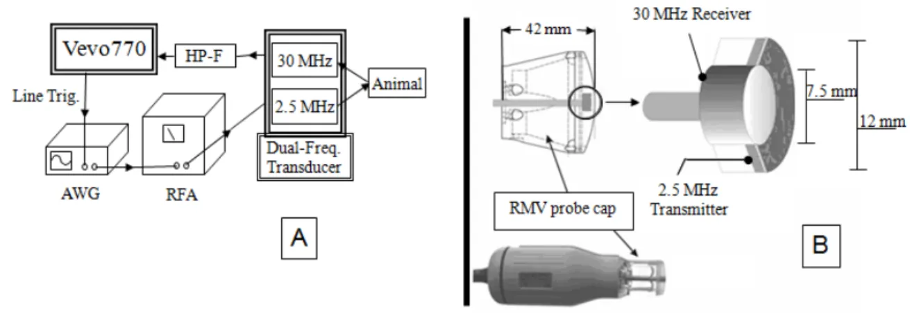
The confocal imaging probe designed by our group is an adaptation of a VisualSonics RMV707 ultrasound probe and is used with a VisualSonics Vevo 770 micro-imaging system, a commonly implemented preclinical ultrasound imaging system. Tradition-ally, the high-frequency piston transducer element within the RMV probe mechanically sweeps to obtain images. An additional 2.5 MHz transducer was added confocally outside the inner 30 MHz element in the adapted setup (Figure 3.1b). This outer low-frequency transducer enabled us to transmit at a low-frequency near microbubble resonance, while receiving the emitted high-frequency signal content with the inner transducer. A schematic displaying how the waveforms were delivered and received by the setup can be seen in Figure 3.1a.
Figure 3.1: (A) Schematic for the operation of the prototype dual-frequency transducer. The arbitrary waveform generator (AWG) (Sony Tektronix) was triggered to send 512 low-frequency pulses through the RF amplifier (RFA) within each frame of image data by the Vevo770 line trigger. (B) A diagram displaying how the two confocal elements were constructed within the RMV probe scanhead.
element receives the reflected ultrasound signal. The unwanted backscatter of tissue is suppressed by sending each line of raw RF data through a seventh-order 10 MHz high-pass filter (HP-F, in the Figure 3.1) (TTE Inc., Los Angeles, CA) before being displayed and saved by the ultrasound imaging system.
Characterizing the probe
spread function of our imaging system and thus determine the practical lateral and axial resolutions achievable in actual ultrasound studies implementing our parameters. Axial and lateral are defined as the parallel and orthogonal directions of wave propagation respectively. Within an image, axial represents the depth axis.
For the first resolution study, a dilute concentration of microbubble contrast agents was pumped through a 27-gauge needle tip coupled to a 380 µm polyethylene tube (Becton Dickinson, Sparks, MD), which was then coupled to a 200 µm capillary tube (Spectrum Labs, Rancho Dominguez, CA) The transducer was set to acquire data with a frame rate of approximately 1 Hz and bubbles were pumped through the capillary tube at 1 mL/h, which corresponded to a linear flow velocity of 9 mm/s. RF data was collected with the 30 MHz element of individual bubble responses for single cycle excitations at 2.5 MHz and at peak negative pressure of 617 kPa. After more than 100 bubble responses were acquired, the time-domain signals were Fourier transformed and averaged together in the frequency domain. Once all pulses had been averaged, the mean frequency-domain signal was then inverse-Fourier transformed to yield a mean time-domain signal. The envelope of this mean signal was determined using Matlab (The MathWorks, Natick, MA), via the absolute value of the Hilbert transform, and the full-width at half-maximum (FWHM) of the envelope used to yield the theoretical limit of the axial resolution for acoustic angiography imaging at our pulsing and receiving parameters.
horizontal cross-sections through this point were extracted from the image data (rep-resenting the axial and lateral components of the point spread function, respectively), interpolated, and the FWHM in each dimension was determined. Thirty samples were collected and averaged. The mean FWHMs in each direction-lateral and axial-were taken as their respective directional resolutions.
Animal and contrast agent preparation
A total of eight Sprague-Dawley rats (Harlan Laboratories, Indianapolis, IN) were im-aged in the course of this study: three during the contrast-to-tissue comparison study and five during the sensitivity to motion study. Before all imaging studies, animals were prepared in the same way. Each animal was first anesthetized in an induction chamber by introducing a 5% aerosolized isoflurane-oxygen mixture. Once sedated, the animal was removed from the induction chamber, the isoflurane concentration reduced from 5% to 2% and maintained via mask delivery. Its abdomen was shaved and a depilating cream was applied to the animal’s skin to dissolve any remaining hair. A 24-gauge catheter was inserted into the animal’s tail vein for the administration of microbub-bles. The animal was then placed in dorsal recumbancy on a heating pad. Finally, ultrasound coupling gel was placed between the imaging transducer and the animal’s skin to ensure the quality of signal transmission. Animals were handled according to National Institutes of Health guidelines and our study protocol was approved by the UNC Institutional Animal Care and Use Committee.
The microbubbles used in this study were the perfusion agent formulation made with a lipid shell and perfluorocarbon core (Appendix A). Contrast agents were diluted in sterile saline to result in a final concentration of 2.2x10⁹ bubbles/mL (unless
Determining contrast-to-tissue ratios
Two studies were performed to examine how imaging pressure affected the probe’s sensitivity to contrast. This sensitivity was quantified with the measure of contrast-to-tissue ratio (CTR). The first study was performed in vitro, and was designed to determine the acoustic responses of both tissue and contrast agents when subjected to the imaging parameters utilized by our probe. The second study was anin vivo study, which compared the CTRs achieved by the probe operating in both high-frequency and acoustic angiography imaging modes within an actual tissue environment.
1) In Vitro CTR Study
For the in vitro CTR study, individual microbubbles in a flow phantom were imaged in acoustic angiography mode at four different mechanical indices (MIs) between 0.33 and 0.57. Bovine muscle tissue was also imaged at the same parameters to simulate the acoustic response of non-perfused tissue. The lines of RF data from these scans were Fourier transformed and divided by the frequency bandwidth of the receiving element. This allowed us to appropriately weight the frequencies in the measured signal which were higher and lower than the probe’s 30 MHz fundamental frequency. By doing this, we were able to compare the spectral power of the true bubble and tissue signals and thus, to compute a theoretical CTR versus frequency plot for multiple imaging pres-sures (regardless of our specific receiving element’s sensitivity).
2) In Vivo CTR Study
AA HF
PNP (kPa) MI PNP (kPa) MI
292 0.18 978 0.18
391 0.25 1318 0.24
492 0.31 1935 0.35
617 0.39 2347 0.43
716 0.45 2792 0.51
814 0.51 3295 0.60
900 0.57 3514 0.64
1030 0.65 3881 0.71
Table 3.1: A Summary of the Imaging Pressures and Mechanical Indices Used in theIn Vivo Contrast-to-Tissue Study for Acoustic Angiography and High-Frequency Imaging Modes.
AA: ‘Acoustic Angiography’ (transmit 2.5 MHz) HF: ‘High Frequency’ (transmit 30 MHz)
of 3 mL/h using a syringe pump (Harvard Apparatus, Holliston, MA). The microbub-ble solution was allowed one minute to reach equilibrium before any image data was collected. Approximately 20 video frames were acquired at 2 Hz in both high-frequency and acoustic angiography modes at each of the six imaging locations. The acoustic an-giography mode was operated with a 2.5-MHz pulsing frequency and a 30-MHz receiver element. The high-frequency imaging mode was operated with pulse-echo only from the 30-MHz element. Both imaging modes used one-cycle sinusoidal driving pulses. Differ-ent image pulsing pressures were evaluated in both imaging modes, as summarized in Table 3.1.
sets collected in each of the kidneys at the different imaging parameters. B-mode im-ages were acquired before and after each administration of contrast agents to ensure consistency of the contrast and tissue ROIs used for each kidney over time (i.e. to ensure they were not corrupted by global shifts in tissue). The mean pixel intensity in the ROIs were calculated at each imaging parameter and compared between animals.
Determining sensitivity to motion
To test the robustness of the acoustic angiography method in the presence of respi-ratory motion, five animals were imaged with power Doppler, image-subtraction, and acoustic angiography imaging modes. The imaging protocol consisted of administer-ing 150 µL bolus injections of microbubble contrast agents, and observing the kidney without respiratory gating as the contrast washed out of the system. The goal was to examine the different imaging modes’ abilities to detect the sharp increase in video intensity following the introduction of microbubbles into the renal volume, as well as their consistency in monitoring the steady decrease in intensity as the contrast agents were cleared from the different animals’ systems. To record the entire contrast washout curve, the left kidney of each animal was imaged for at least 6 min following each injection. All three imaging modes were tested within the same anatomical region of each animal (meaning neither the animal nor the transducer was moved between data acquisitions with different imaging modes). Following the collection of data, videos were exported and examined offline in Matlab for analysis of these curves.
Production of radiation force
The ability of the dual-frequency probe to produce radiation force was tested in vitro
with the corresponding linear flow velocities.
V-FR (mL/h) L-FR (mm/s) Analogous environment
9.05 200 Large artery
1.81 40 Small artery
1.81 40 Large vein
0.90 20 Arteriole
0.45 10 Small vein
0.14 3 Venule
0.01 0.3 Capillary
Table 3.2: A summary of the range of blood velocities in different vasculature types. Modified from [71]. These velocities formed the basis for the tested range of flow velocities of contrast agents undergoing radiation force.
V-FR: ‘Volumetric flow rate’ L-FR: ‘Linear flow velocity’
3.1.2 Results
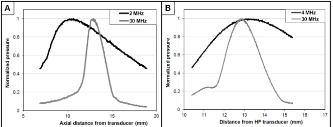
Characterizing the probe
Figure 3.3: Axial dimension pressure maps for both (A) first generation and (B) second generation dual-frequency transducers.
Contrast-to-tissue ratios: in vitro
The acoustic responses of both bubbles and tissue were used to create a measure of CTR versus receive frequency at several different mechanical indices for the imaging pulses. To illustrate the difference between the types of signals received from microbubbles and from tissue, time domain plots are provided (Figure 3.4). These data were acquired using the maximum transmit mechanical index for the study (MI = 0.65).
To illustrate the frequency domain characteristics of these data, the Fourier trans-formed data are provided (Figure 3.5) with the receive transducer’s bandwidth super-imposed for reference.
Figure 3.5: Frequency responses of the single lines of microbubble (blue) and tissue (red) RF data seen in Figure 3.4. The transducer’s receive bandwidth is approximated as a Gaussian with 100 percent bandwidth centered at 30 MHz.
Figure 3.6: (A) Contrast-to-tissue ratios measured in vitro as a function of frequency at several different mechanical indices of incident pulses. Decibel values are relative to the tissue response at each frequency and MI. (B) Contrast-to-tissue ratios measuredin vivo in six different kidneys which were imaged in both high-frequency b-mode (dashed line) and acoustic angiography mode (solid line).
Contrast-to-tissue ratios: in vivo
The video data collected from contrast enhanced ultrasound studies on both kidneys of three different animals in both traditional high-frequency b-mode and acoustic an-giography imaging modes were analyzed to determine CTR in anin vivo environment. Both a 2D slice and a 3D maximum intensity projection of a kidney imaged in acoustic angiography mode can be seen in Figure 3.7, providing a representative view of the extent of tissue suppression provided by this imaging method. In a 2D image slice of each kidney, ROIs were selected around regions of tissue and contrast for both the acoustic angiography and high-frequency imaging studies, and these values were used to determine the CTR at each imaging pressure. These values are plotted in Figure 3.6b.
Figure 3.7: (A) A 2D transverse slice through a rat kidney with contrast agents seen entering the volume through the large renal vasculature. (B) A 3D maximum intensity projection through a rendered volume of sequential image slices as seen in (A). The multiple 2D slices were acquired using a translational motor stage with step sizes of 200 µm. The images analyzed in the CTR portion of this study were identical to the cross-sectional slice seen in (A).
Sensitivity to motion
Within the seven sets of image data collected in five different animals with power Doppler, image subtraction, and acoustic angiography imaging modes without respira-tory gating, acoustic angiography imaging was significantly more robust at monitoring the presence of microbubbles. Because of the artifacts in the video data resulting from respiratory motion, the image-subtraction method was unreliable without respiratory gating. In this mode, the changes in video intensity caused by tissue motion were approximately the same amplitude as the signal from the circulating contrast, and we were only able to observe a decay slope of the contrast washout in the kidney ROI in one of the animals.
Similarly, 5 of 7 imaging studies using power Doppler were corrupted to the point that a washout curve could not be acquired. Examples of how these imaging modes were corrupted by breathing motion can be seen in Figure 3.8. In contrast, the acous-tic angiography imaging experiments (N = 7) produced a defined contrast washout curve in each case despite substantial respiratory motion. Figure 3.9 illustrates the relative success rates for the different imaging strategies, with acoustic angiography mode demonstrating a 3.5- and 7-fold improvement over power Doppler and image-subtraction, respectively.
Production of radiation force
Figure 3.8: Example image data collected from the same animal without respiratory gating enabled. (A) B-mode imaging before the introduction of contrast agents. (B) Acoustic angiography data while contrast is circulating. (C) Image-subtraction frame while contrast is circulating. Note the strong artifacts near the tissue borders (indicated by white arrows). (D) Power Doppler with contrast circulating. Small regions of enhanced contrast can be seen near the bottom of the image, although most of ROI is washed out by motion artifact.
different linear flow velocities between 0.3 and 200 mm/s, as summarized in Table 3.2. The radiation force pulses from the probe were able to divert the flow of contrast agents a distance of 200 µm-the diameter of the tube-at all linear flow velocities less than 50 mm/s. At flow rates faster than this, the direction of the microbubble stream was perturbed, though did not significantly divert within the viewing window of 500 µm. At 200 mm/s, the stream was only estimated to divert approximately 50 µm at
Figure 3.9: A plot comparing the abilities of the three different imaging modes to monitor contrast flow in the presence of respiratory motion. Values are expressed as a percentage of the seven attempted trials. Note: ‘Dual-frequency’ = acoustic angiogra-phy
Potential for bioeffects
The interactions between ultrasound pulses and microbubble contrast agents have been shown in the past to potentiate bioeffects, both in in vitro assays as well as in vivo
Figure 3.10: A time-axis projection image produced from bright-field optical video data, which demonstrates the proficiency of the dual-frequency probe at diverting a moving stream of microbubbles. The linear flow velocity in this image was 40 mm/s, a comparable speed to a human small artery or large vein.
3.1.3 Discussion
Based upon the work of Kruse et al. [66], we hypothesize that the high-frequency energy that we are detecting from the microbubbles is generated during the rapid collapse of the gas core during the low-frequency driving pulse. In the frequency domain, these emitted acoustic transients were confirmed to be very broadband, as seen in Figure 3.6a, allowing them to be detected at frequencies far away from the fundamental.
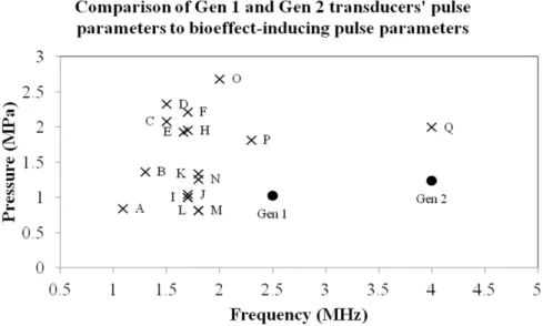
Figure 3.11: An overview of bioeffect-inducing acoustic parameters. These studies are referenced as follows. A:[72], B:[73], C:[74], D:[75], E:[76], F:[77], G:[78], H:[79], I:[80], J:[81], K:[82], L:[83], M:[84], N:[85], O:[86], P:[87], Q:[85].
µm compared with the high-frequency element’s 16 µm. There were several
conse-quences of this misalignment. One issue with this was that the focus of the 30-MHz element overlapped the 2.5-MHz element approximately -6 dB from the focus, and hence the signal intensity from the microbubbles detected during acoustic angiography mode was substantially less than optimal. One other consequence was that the mi-crobubbles were rapidly destroyed outside of the imaging region because of a higher pressure at the focus of the misaligned 2.5-MHz transducer. This resulted in differences in the contrast intensity depending on whether the transducer was scanning with the focus of the 2.5-MHz element preceding or following the imaging element.
For all imaging pressures tested, the CTR versus frequency curve peaked at approx-imately 15 MHz, and decreased from there with increasing frequency (Figure 3.6). This decline in CTR was caused by the decrease in spectral power of the acoustical tran-sients at the higher frequencies, because the spectral power of the tissue signal quickly approached the noise floor above the fundamental imaging frequency of 2.5 MHz. The CTR increased uniformly across all frequencies in the bandwidth of the receiving ele-ment with increasing imaging MI, which can be attributed to more violent collapses of the microbubble gas cores at increasing pressures.
The results obtained during the in vivo CTR portion of the study showed that the acoustic angiography imaging method could be used in animal studies to improve contrast sensitivity over conventional high-frequency imaging methods. High-frequency b-mode imaging showed little improved contrast signal over tissue signal regardless of imaging pulse pressure. The average CTR in high-frequency b-mode was 1.18. Acoustic angiography imaging of the same animals and the same imaging locations showed a linearly increasing trend in average CTR ranging from 1.3 to 4.8, increasing as a function of increasing imaging pressure. After approximately 800 kPa, the rate of increase in the contrast signal was similar to that of the tissue signal and the CTR did not noticeably improve at higher imaging pressures.
There was an approximately 10-fold difference between the in vitro and in vivo
information inherent in any imaging system’s compression and video-data display al-gorithms. Instead, this data served to provide a basic understanding of the acoustic responses of microbubbles and tissue at frequencies higher than previously examined.
In Figures 3.7 and 3.8b, it is clear that the larger vasculature within the kidney is brighter and better delineated from the surrounding tissue than smaller blood vessels. Thus the contrast provided by our acoustic angiography imaging method appears to be, predictably, a function the quantity of contrast agents present within the imaging ROI. If the probe is to be operated within a destructive pressure regime for microbubbles (a range which provided the best contrast within our in vivo CTR study [88]), one potential limitation of our imaging strategy would be the need to delay imaging pulses to allow contrast refresh within the micro-vasculature. This decreased frame rate would be beneficial for imaging tissues with slow perfusion times.
because global tissue migration will invalidate the original pre-contrast baseline images. Acoustic angiography imaging, on the other hand, exploits the nonlinear response of microbubbles to enhance contrast signal intensity and thus proved significantly more robust in the presence of respiration-induced tissue motion than either power Doppler or image-subtraction methods.
Although not shown here, we were able to generate overlays of contrast data over the b-mode tissue by utilizing a relay circuit to toggle excitation of the low-frequency and high-frequency elements with successive imaging frames, and then displaying successive tissue and contrast frames together by color coding the contrast data.
Based on the results of thein vitro radiation force experiments, the dual-frequency probe could be utilized to direct microbubbles to the endothelial wall in targeted imag-ing studies over a range of physiologically relevant flow velocities. Additionally this ability could be implemented in acoustically-mediated drug delivery studies, because the probe is also capable of delivering acoustic energy above the bubble destruction threshold, which would facilitate site-specific release of therapeutic agents.
3.1.4 Conclusion
We have demonstrated that acoustic angiography imaging can be utilized in vivo at higher frequencies than previously demonstrated to produce high-resolution images with high contrast-to-tissue ratios. Because of the substantial tissue suppression, this technique is robust in the presence of tissue motion. Additionally, the probe effectively produced radiation forcein vitro on microbubbles with flow-rate parameters analogous to most types of environments found within a wide range of vasculature types.
3.2 High resolution assessment of vessel architecture - ex vivo tissue sam-ples
immunosuppressant treatments associated with liver transplants. Thus, it is these ex-tracellular matrix scaffolds prepared from decellularized tissues that are the hope for stable organoids. Ongoing efforts are focused on establishing human liver organoids by seeding liver biomatrix scaffolds with stem cells, hHpSCs10 or biliary tree stem cells11, and with their mesenchymal cell partners (angioblasts and precursors to endothelia and hepatic stellate cells)[91].
internal flow. This approach can be useful for identifying insufficient flow within large regions in the sample, such as throughout an entire lobe, but it is insensitive in detect-ing subtle variations in volumetric perfusion over time. Thus a method to image both the anatomy and flow within the sample is highly desirable. Hence, in these studies, we have developed a protocol to enable rapid yet detailed assessment of vascular structural and functional characteristics within liver biomatrix tissue scaffolds.
Imaging methods for assessing tissue engineering scaffolds
There are many methods used to image tissue scaffolds, including scanning and trans-mission electron microscopy (SEM and TEM) and optical microscopy[93], magnetic resonance (MR) imaging and microscopy [94], computed tomography (CT) [95], opti-cal coherence tomography (OCT) [96], and Doppler ultrasound[97]. The selection of any one modality will always yield inherent tradeoffs, such as cost, invasiveness to the sample, field of view, resolution, acquisition time, and type of information gleaned. For an extensive assessment of the tradeoffs, the reader is referred to a review by Mather [98]. The only imaging modalities in the above list which can holistically (i.e. image a sample in its entirety) and non-invasively image a rodent tissue biomatrix scaffold sample in its entirety are MR, CT, and ultrasound. MR and CT are widely available in both clinical and research contexts, though require expensive hardware, are not real time, require long image acquisition times (MR), can cause radiation damage to cells (CT), and suffer from poor soft tissue contrast (CT). Ultrasound, on the other hand is real-time, relatively inexpensive, non-invasive, does not use ionizing radiation, and has excellent soft-tissue contrast. In addition to these, ultrasound is able to assess multiple different facets of a tissue volume (applicable to both in vivo volumes and
speed[31]. One possible challenge hindering ultrasound’s utility for scaffold perfusion assessment has likely been the modality’s limited field of view, allowing for freehand visualization of different 2D slices, or small 3D sub-volumes, but never holistic visual-ization or quantitation. Our objective in this study was to design a tissue preparation, restraint, and imaging protocol to enable the 3D visualization and quantification of perfusion throughout a biomatrix scaffold.
Contrast ultrasound imaging
quantitation, and then mapping perfusion rates with flash replenishment. Note that all three studies could be performed sequentially with appropriate system hardware.
3.2.1 Materials and methods:
The scaffold preparation procedure is provided in Appendix C.
Sample imaging chamber
Figure 3.12: Schematics for the sample imaging chamber. A) Assembled sample imag-ing chamber and B) exploded view of the sample imagimag-ing chamber. C) A top-down cartoon schematic illustrating the two flow circuits in the setup. Flow Circuit 1 pro-vided perfusion and microbubbles to the liver scaffold, while Flow Circuit 2 propro-vided continuous circulation through the microbubble sequestration and destruction chamber (MSDC) to remove contrast excreted from the sample.
prevent this, a bubble clearance fluid circuit was implemented (Flow circuit 2 in Figure 3.12C). This circulated the fluid surrounding the scaffold sample though a microbub-ble sequestration and destruction chamber (MSDC) before reinjection back into the imaging chamber. The MSDC was a 2 L Erlenmeyer flask in which was suspended a 1 MHz unfocused piston transducer (Valpey-Fisher - Hopkinton, MA) designed to facil-itate contrast destruction. The 1 MHz piston transducer was pulsed at 10 Hz with a pressure of 460 kPa via a pulser (Model 801A, Ritec - Warwick RI). Media surrounding the biomatrix scaffold was continually pumped through this chamber at 1 mL/min via a centrifugal pump (model PQ-12, Greylor - Cape Coral, FL) powered by an external DC power supply (model DIGI360, Electro Industries - Westbury, NY). Four nylon luer fittings were attached to the outer cylinder for coupling the sample imaging chamber to the two flow circuits. All fluid circuits used 0.125 inch inner diameter Tygon tubing, except between the catheter entering the scaffold sample and the outer cylinder of the imaging chamber: this was 0.062 inch diameter tubing.
Contrast imaging
Acoustic angiography was performed on the second generation dual-frequency probe described in Chapter 3.1 with imaging parameters previously described [101]. Briefly, the imaging system was a VisualSonics Vevo770 (Toronto, ON, Canada) pulses were emitted at 4 MHz at 1.23 MPa, and echoes were received on a 30 MHz transducer with 100% bandwidth after being passed through a 15 MHz high pass filter to remove non-contrast signal. 3D images were acquired with the VisualSonics 1D motion stage with inter-frame distance of 100 µm to yield nearly isotropic voxels. Images were acquired with a frame rate of 2 Hz, with 5 frames averaged at each location. High resolution b-mode images were also acquired on the Vevo770 system with the same imaging parameters, except the transmit frequency changed to 30 MHz. After imaging, data was exported from the ultrasound system as 8 bit uncompressed AVIs.
The microbubbles used in this study were prepared with the Perfusion Agent formu-lation as described in Appendix A. Microbubbles were introduced to the perfusion fluid circuit through a T-valve injection port located between the pulse dampener and the biomatrix. A 24 gauge needle was used to pierce the septum, and microbubbles could then be injected into the fluid circuit via a computer controlled syringe pump (Harvard Apparatus - Holliston, MA). Microbubbles were administered into the fluid circuit at a rate of 20 µL min−1 and concentration of 1.5x10⁹ mL−1 out of a 1 cc syringe.
axial field of view. Each liver biomatrix scaffold was imaged with two imaging modes: flash replenishment, and acoustic angiography.
Validating imaging consistency
Registration of sub-volumes
Because the lateral field of view of the ultrasound transducers used for these imag-ing studies was insufficient to capture the entirety of the liver lobe of interest, multi-ple “sub-volumes” were acquired on each system and later registered together offline. Throughout this manuscript, sub-volume is used to describe a 3D volumetric image that does not holistically capture a tissue of interest. Registration of these sub-volumes was performed within the open source 3D Slicer environment (ver 4.2.1, National Alliance for Medical Image Computing - www.slicer.org) using the Merge module, part of the TubeTK extension. This module is designed to register together two images that have a small degree of overlap along one of the axes. When the sub-volumes were registered together using the Merge module, they would form a single cohesive volume for the liver lobe of interest for each image type (b-mode, flash replenishment, and acoustic angiography). The transforms module was used to then register the three types of ultrasound image data to each other, creating a single composite 3D image for each of the livers imaged.
Assessing liver biomatrix perfusion
not imaged. In these cases, ROIs were defined to the edge of the available image data, or across regions of tissue if it was obvious to the viewer what path the tissue boundary was taking.
Each voxel within the flash replenishment images represented a spatially localized estimate of perfusion speed. To assess perfusion throughout the volume of tissue, all values were vectorized and histograms were created for each sample. These perfusion histograms were binned by perfusion time, and area normalized by total perfused voxels (i.e. the integral of the histogram was set to unity). To segment the vessels out of the acoustic angiography datasets, a previously described segmentation algorithm was used [51]. These segmentations were used to compute total length and volume of the vessel network, vascularity ratio (volume of vessel network/volume of liver lobe). The volume of each discretized location in the segmented vessel network was computed and summed to yield total vessel network volume and length. The proportion of the vessel network occupied by vessel segments of a range of radii between 50 µm (minimum voxel size) and 500 µm was computed.
3.2.2 Results
Validation of imaging consistency