DOI:10.1051/0004-6361/201526719 c
ESO 2016
Astrophysics
&
Weak-lensing-inferred scaling relations of galaxy clusters
in the RCS2: mass-richness, mass-concentration, mass-bias,
and more
Edo van Uitert
1,2,3, David G. Gilbank
4, Henk Hoekstra
2, Elisabetta Semboloni
2,
Michael D. Gladders
5, and Howard K. C. Yee
61 Argelander-Institut für Astronomie, Auf dem Hügel 71, 53121 Bonn, Germany e-mail:[email protected]
2 Leiden Observatory, Leiden University, Niels Bohrweg 2, 2333 CA Leiden, The Netherlands 3 University College London, Gower Street, London WC1E 6BT, UK
4 South African Astronomical Observatory, PO Box 9, 7935 Observatory, South Africa
5 The Department of Astronomy and Astrophysics, and the Kavli Institute for Cosmological Physics, The University of Chicago, 5640 South Ellis Avenue, Chicago, IL 60637, USA
6 Department of Astronomy and Astrophysics, University of Toronto, 50 St. George Street, Toronto, Ontario, M5S 3H4, Canada
Received 11 June 2015/Accepted 12 October 2015
ABSTRACT
We study a sample of∼104galaxy clusters in the redshift range 0.2< z <0.8 with massesM
200 >5×10¹³h−701 M, discovered in the second Red-sequence Cluster Survey (RCS2). The depth and excellent image quality of the RCS2 enabled us to detect the cluster-mass cross-correlation up toz ∼0.7. To obtain cluster masses, concentrations, and halo biases, we fit a cluster halo model simultaneously to the lensing signal and to the projected density profile of red-sequence cluster members, because the latter provides tight constraints on the cluster miscentring distribution. We parametrised the mass-richness relation asM200 =A×(N200/20)αand findA=(15.0±0.8)×1013h−1
70 Mandα=0.73±0.07 at low redshift (0.2<z<0.35). At intermediate redshift (0.35<z<0.55), we find a higher normalisation, which points towards a fractional increase in the richness towards lower redshift caused by the build-up of the red sequence. The miscentring distribution is well constrained. Only∼30% of our BCGs coincide with the peak of the dark matter distribution. The distribution of the remaining BCGs are modelled with a 2D-Gaussian, whose width increases from 0.2 to 0.4h−1
70Mpc towards higher masses. The ratio of width andr200is constant with mass and has an average value of 0.44±0.01. The mass-concentration and mass-bias relations agree fairly well with literature results at low redshift, but have a higher normalisation at higher redshifts, possibly because of selection and projection effects. The concentration of the satellite distribution decreases with mass and is correlated to the concentration of the halo.
Key words.gravitational lensing: weak – galaxies: clusters: general
1. Introduction
Observations of galaxy clusters provide a wealth of astrophysi-cal and cosmologiastrophysi-cal information. A key quantity of clusters is the mass, because it determines the relative importance of vari-ous processes such as AGN feedback. Furthermore, given a large sample of cluster masses, the cluster mass function can be deter-mined and compared to simulations in order to constrain cos-mological parameters, such as the normalisation of the matter power spectrum,σ8, and the cosmological matter density,ΩM
(e.g.Evrard 1989;White et al. 1993); if the redshift baseline of the sample is sufficiently large, the dark energy equation of state can be constrained (e.g.Voit 2005;Allen et al. 2011).
The mass of a cluster is not a direct observable, but can be determined with a variety of techniques. The velocity dis-tribution of cluster members has been used to derive dynam-ical mass estimates (e.g. van der Marel et al. 2000; Łokas et al. 2006), but these observations are generally expensive since they require spectroscopic observations of many cluster members. Additionally, assumptions on the satellite orbits are needed to convert the velocity dispersions into a mass esti-mate. X-rays observables can also be used to estimate the mass
(seeEttori et al. 2013, for a review), under the assumption that the hot cluster gas is in hydrostatical equilibrium. The results of Mahdavi et al. (2008, 2013) support the results from hy-drodynamical simulations (e.g.Nelson et al. 2014) that clusters are generally not in hydrostatical equilibrium, which biases the X-ray-based mass estimates. Another powerful method of ob-taining cluster masses is weak gravitational lensing.
In weak lensing, the distortion of the images of faint back-ground galaxies (sources) due to the gravitational potentials of intervening structures (lenses) is measured. This signal is pro-portional to the excess surface mass density, which can be mod-elled to obtain the mass. Weak lensing does not rely on direct tracers of the potential; the distortion can be measured for any lens, out to large radii where no visible tracers can be used. Additionally, the weak lensing signal does not depend on the physical state of the matter in the clusters, and no assumptions have to be made (e.g. virial equilibrium) to measure the total pro-jected mass. Weak lensing has been used to determine the mass of individual massive low-redshift clusters (e.g.Hoekstra 2007; Okabe et al. 2010;Hoekstra et al. 2012,2015;Applegate et al. 2014;Gruen et al. 2013;Umetsu et al. 2014;Kettula et al. 2015),
as well as the average mass of samples of clusters and galaxy groups by stacking their lensing signals (e.g.Mandelbaum et al. 2006a;Sheldon et al. 2009;Covone et al. 2014;Ford et al. 2015). From the weak-lensing signal, many cluster properties can be extracted, such as the cluster mass, concentration, halo bias, and miscentring distribution. The relation between these param-eters can help constrain models of cluster physics. To determine the mass function, however, we need mass estimates of a large number of clusters. The lensing signal of all but the most massive clusters is generally noisy; only by stacking the signal of sam-ples of clusters can the average mass be robustly constrained. A common solution is to determine how an observable cluster property scales with mass and can serve as a mass proxy. The Sunyaev-Zeldovich effect has been used (e.g.Williamson et al. 2011) and appears particularly useful for estimating the masses of massive clusters at high redshifts through scaling relations. Another observable property is the richness, which has the ad-vantage that it can be determined from the same multi-colour imaging data that is used for the lensing analysis.
To determine the richness of a cluster, it is necessary to distinguish cluster galaxies from fore- and background galax-ies and, if necessary, correct for contamination. Cluster mem-bers can be identified if their redshift or velocity dispersions are available, which requires either spectroscopy or observations in many bands for reliable photometric redshifts. Alternatively, cluster members can be identified using their colours as the ma-jority of early-type galaxies in a cluster populate a narrow range in colour–magnitude space, that is, the E/S0 ridge line or the red sequence (Gladders & Yee 2000). The advantage of the lat-ter is that observations in only two bands suffice, which makes it cheap and particularly suited for the automated detection of clusters in large imaging surveys (e.g.Gladders & Yee 2005). Additionally, only a few field galaxies reside in this regime of colour–magnitude space, which reduces the contamination.
In this paper we use optical imaging data from the second Red-sequence Cluster Survey (RCS2;Gilbank et al. 2011), both to detect clusters and determine their richness, as well as to mea-sure their lensing signals. The survey design was chosen so as to optimise the detection of a large number of clusters using a red-sequence method (Gladders & Yee 2000). In total,∼104
clus-ters have been detected in the RCS2, spread over a wide range in optical richness, with redshifts 0.2 < z < 0.9. In contrast, the maxBCG cluster sample (Koester et al. 2007), a catalogue of 13 823 clusters that has been detected in the Sloan Digital Sky Survey (SDSS;York et al. 2000), covers a redshift range of 0.1 < z < 0.3, which limits its use for evolutionary stud-ies. The redshift range of clusters in the RCS2, combined with the excellent lensing quality of the data, makes the RCS2 well suited to this purpose.
The outline is as follows. In Sect.2, we present the vari-ous steps of the analysis: we discuss the cluster detection and richness estimates (2.1), provide details of the lensing measure-ment (2.2), and discuss our halo model (2.3). We highlight our novel approach of including the cluster-satellite correlation to constrain the miscentring distribution in Sect.2.3.1. We present the mass-richness relation in Sect.3, the cluster miscentring dis-tribution in Sect.4, the mass-concentration relation in Sect.5, the satellite distribution in Sect.6and the mass-halo bias rela-tion in Sect.7. We conclude in Sect.8. Throughout the paper we assume a WMAP7 cosmology (Komatsu et al. 2011) with
σ8 = 0.8,ΩΛ = 0.73,ΩM = 0.27,Ωb = 0.046 and h = 0.7
the dimensionless Hubble parameter. All distances quoted are in physical (rather than comoving) units unless explicitly stated otherwise.
2. Analysis
The RCS2 is a nearly 900 sq. deg imaging survey in three bands (g, randz) carried out with the Canada-France-Hawaii Telescope (CFHT) using the one square degree field of view camera MegaCam. The primary imaging data covers 740 sq. deg of sky, divided in 13 patches. The survey area can be split into 145 blocks of contiguous non-overlapping 2 ×2 deg of sky, which we use to estimate the bootstrap covariance matrices of our measurements as discussed later on. Hence in total we use 580 sq. deg. The lensing analysis is performed on the eight minute exposures in ther-band (rlim ∼ 24.3), which is best suited for lensing with a median seeing of 0.71.
The photometric calibration of the RCS2 is described in de-tail inGilbank et al.(2011), the lensing analysis in van Uitert et al. (2011). For details, we refer the reader to these works. In short, we measured the shapes of 2.2×10⁷ galaxies using
the KSB method (Kaiser et al. 1995;Luppino & Kaiser 1997; Hoekstra et al. 1998, 2000), which corresponds to a source number density of 6.3 arcmin−2. Two major improvements to the lensing analysis were introduced inCacciato et al.(2014), van Uitert et al.(2015): we used the photometric redshift cata-logues fromIlbert et al.(2013) instead of the catalogues from Ilbert et al.(2009) to estimate the source redshift distribution; and secondly, we introduced a correction scheme to account for a multiplicative bias in our KSB method (due to noise bias (Kacprzak et al. 2012;Melchior & Viola 2012;Refregier et al. 2012), and galaxy blends), which affects the lensing measure-ment (Hoekstra et al. 2015).
2.1. Cluster detection
Galaxies clusters are identified using a modified version of the algorithm presented inLu et al.(2009). This is a simplified ver-sion of theGladders & Yee(2005) red-sequence cluster-finding method. The main modifications are described in Gilbank et al. (in prep.), detailing how the method was applied to RCS2 data. Briefly, the significance of a candidate cluster overdensity is de-termined from a count of (colour-selected) galaxies within a cir-cle with a radius of 0.5 Mpc. Unlike theGladders & Yee(2005) method, no magnitude weighting is applied to the galaxies, and the uncertainties in the cluster and field counts are estimated di-rectly from Poisson statistics. Colour slices are built at regular colour intervals (which leads to irregular bins in photometric redshift), and each slice overlaps its neighbour by a quarter of the slice width. For RCS2, the method is identical except that the model colour–redshift relation was transformed to the RCS2 fil-ters. One additional modification for RCS2 involves the centring adopted, which aims to locate the BCG via a simple two-step approach, as discussed in AppendixA.
Richnesses are estimated using an approach similar to the one outlined inKoester et al.(2007),Hansen et al.(2005,2009), and Johnston et al. (2007) for the maxBCG cluster sample. Firstly, the number of red-sequence galaxies brighter thanM+1 within an aperture of radius one Mpc is counted.Mis estimated from simple stellar population synthesis models, as described in Lu et al.(2009). This count is then used to estimater200 (the
radius inside of which the density is 200 times the critical den-sity,ρc) for each cluster using the relationrgal200=0.156Ngal0.6Mpc
fromHansen et al.(2005). The number of red-sequence candi-dates brighter thanM+1 withinrgal200givesN200, our richness
estimate. Since we also apply a background subtraction,N200are
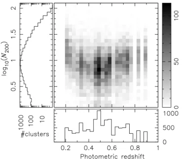
Fig. 1.Redshift versus log10(N200), the logarithm of the number of early-type cluster members brighter thanM+1 insidergal200. The clusters cover a wide range in richness and redshift, and are therefore very well suited to studying the redshift dependence of the mass-richness relation.
The maxBCG papers listed above use a variety of slightly different scaling relations which vary in both exponent and nor-malisation depending on precisely howr200was derived. The
re-lation we choose is similar to that given inHansen et al.(2005), although their radius is quoted inh−1
100Mpc and here we do not
correct for the different cosmology, given the range of values in the normalisation from method-to-method. In practise, a diff er-ent normalisation should just lead to counting within a different fraction ofr200. Therefore, mass–richness estimates within a
sin-gle cluster sample should still be internally self-consistent, and to compare between samples it should suffice to apply a constant systematic scaling.
The distribution of cluster redshifts and richnesses are shown in Fig.1. To assess the accuracy of the “red-sequence” redshifts, we match the BCGs to the galaxies with spectroscopic redshifts from the ninth data release of the SDSS (DR9;Ahn et al. 2012). In total, we find 2212 matching galaxies. We compare the red-shifts in Fig.2 and find that they agree quite well. Note that the stripes of “red-sequence” redshifts reflect the redshifts slices used to detect the clusters. Only at redshifts belowz<0.3 and abovez>0.7, the “red-sequence” redshifts are slightly overes-timated. The average difference in each redshift slice is shown in Fig.3. At low redshift, the bias is likely the result of only us-ing red-sequence templates up toz =0.248; at lower redshifts, the colours become degenerate. The cause of the bias atz>0.7 is less obvious, but seems to indicate that the initial calibration of the red-sequence templates using spectroscopic data was af-fected by outliers (either mismatches or matches that sampled re-gions with poorer than average photometry). We examined these clusters in detail and decided there was no obvious reason to re-ject them from the analysis. We correct the cluster redshifts for this bias by fitting a third-order polynomial to these matching galaxies, and apply the same shift to all our clusters. The rich-nesses are recomputed using the corrected redshifts. Note that Fig.1shows the corrected redshifts and the corrected richnesses, the quantities used in this work.
After correcting the redshift bias, we compute the scatter and show it in the lower panel of the same figure. When we
Fig. 2.Comparison of our “red-sequence” redshifts to the spectroscopic
redshifts from SDSS.
Fig. 3.Mean difference between our “red-sequence” redshifts and the
spectroscopic redshifts from SDSS (top). Scatter between the redshifts after accounting for the bias (bottom). Open symbols indicate the scat-ter for all matches, solid ones are obtained afscat-ter removing the outliers (|zRCS2−zSDSS|>0.15). The dashed/dotted-dashed line shows the mean scatter including/excluding outliers. We correct the mean redshift bias in our analysis.
remove obvious outliers using |zRCS2 −zSDSS| > 0.15, which
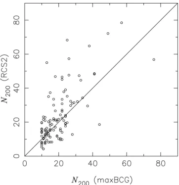
Fig. 4. Comparison of the cluster richnesses of 114 matched clus-ters from maxBCG and RCS2. The solid line shows the one-to-one relationship.
determined because of the low number of matches. For this work that is not important, as we restrict our analysis to clusters withz<0.8.
To evaluate our richness estimates, we match our clusters to the maxBCG catalogue. We find 114 matches and compare the N200 estimates in Fig. 4. The richnesses of clusters in the
RCS2 appear systematically larger at the high-richness end. This may partly be attributed to an improved deblending in the RCS2 because of the better observing conditions. The scatter between the estimates is quite large, part of which may be attributed to particular settings in the cluster detection algorithm that deal with mergers and projections on the sky.
Not all detections in the cluster catalogue are real clusters: a fraction of the clusters may actually correspond to a chance pro-jection of galaxies rather than to a real cluster. These false de-tections have presumably a different lensing mass than the real clusters of that richness, but since both the richness and mass are affected simultaneously, the bias on the scaling relation is expected to be small. The fraction of real clusters is called the purity, which is generally a function of richness and redshift, but also depends on the cluster detection algorithm. Therefore, to de-termine the actual value of the purity for our cluster sample, we need to apply the detection algorithm to mock data that mimic the RCS2, which has not yet been done. The false positives do not add random noise, but a coherent (but likely lower) lensing signal. How large the impact is on the lensing mass, needs to be addressed with simulations. Note that the detection significance in our cluster finder is high, favouring a high purity over a high completeness.
Figure1shows that our cluster sample is incomplete at the low richness end. In principle, this should not affect our results, as the average lensing signal only becomes noisier if we miss clusters in our sample. However, to use the cluster sample to constrain cosmological parameters, a detailed knowledge of the completeness function is a prerequisite.
2.2. Lensing measurement
The shapes of source galaxies are distorted by the gravitational potentials of clusters. In the regime where the surface mass den-sity is sufficiently small, the gravitational shear can be approxi-mated by averaging the ellipticities of source galaxies (for a re-view of cluster lensing, seeHoekstra et al. 2013). We determine the tangential component of the shear in radial bins centred on the BCGs,
γt(r)= ΔΣ
(r) Σcrit
, (1)
which is related to the surface density contrast,
ΔΣ(r)=Σ¯(<r)−Σ¯(r), (2) the difference between the mean projected surface density en-closed byrand the mean projected surface density at a radiusr. The shear signal at small scales around massive clusters is so large that it no longer can be approximated as being linearly re-lated to the galaxy ellipticities. We accounted for this when we computed the models (see Sect.2.3).Σcritis the critical surface
density: Σcrit=
c2
4πG Ds
DlDls
, (3)
withDl, Ds andDls the angular diameter distance to the lens,
the source, and between the lens and the source, respectively (Bartelmann & Schneider 2001). Since we lack redshifts for the sources, we select galaxies with 22<mr <24 that have a
reli-able shape estimate (ellipticities smaller than one, no SExtractor flag raised) as our source sample. To determine their approxi-mate redshift distribution, we apply identical magnitude cuts to the publicly available photometric redshift catalogue of Ilbert et al.(2013). We use this redshift distribution to compute the mean lensing efficiency,Dls/Ds, as a function of lens redshift,
accounting for the changing average weight of the sources as a function of apparent magnitude, and accounting for the im-pact of outliers in the catalogue. This procedure is outlined in Appendix C ofCacciato et al.(2014).
In Appendix B ofvan Uitert et al.(2015), we present a test of the robustness of our measurement algorithm. In short, we mea-sure the lensing signal using different source magnitude cuts, and for each cut we recompute the lensing signal (after deriving new lensing efficiencies, random signals, noise bias corrections and source galaxy contamination corrections). Both at low and high redshifts, the resulting lensing measurements are consis-tent, suggesting that this method of measuring tangential shear is robust.
Here we present results from an additional test. Since we only select galaxies with a flux radius that is at least 10% larger than the local PSF size, it is possible that we systematically re-move the smallest, highest redshift galaxies from our analysis; we do not account for that when we compute the lensing effi -ciencies, which could potentially lead to biases. We check that by removing the 10% smallest objects (in terms ofrh) from the
photo-zcatalogues ofIlbert et al.(2013), and recompute the lens-ing efficiencies. At low lens redshifts, the results are practically unchanged. Atz = 0.7, the highest mean lens redshift that we study in this work, the lensing efficiencies only decrease by 3%. Removing the smallest 40% of objects (much more than we do in practice) leads to a decrease of 8%. Hence the effect is not completely negligible, but it is smaller than our statistical errors and unlikely to lead to a significant bias.
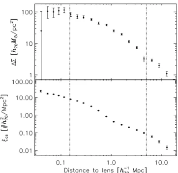
Fig. 5.Stacked lensing signal (top) and cluster-satellite correlation ( bot-tom) measured for all clusters withN200 > 2 and 0.2 < z < 0.8 in the RCS2. The vertical dot-dashed lines indicate the fitting range for the cluster halo model. Both measurements are shown for illustration only.
As mentioned before, the cluster redshifts have been cor-rected for a mean bias. This correction is uncertain for redshifts larger than 0.8 due to the low number of matches. Hence we restrict ourselves to clusters atz < 0.8. The scatter of the lens redshifts also affects the lensing measurement. We estimate the effect in AppendixB, and find that the impact on the lensing signal is at the per cent level. Therefore, it can be safely ignored. The distortions induced by weak lensing are much smaller than the intrinsic ellipticities of the sources. The lensing mea-surement of a single cluster is therefore generally very noisy. To improve the signal-to-noise, the lensing signal is stacked for a sample of clusters that have similar properties (e.g. within a certain richness range). Stacking the lensing signal has the ad-ditional advantage that the contribution from uncorrelated struc-tures, as well as from potential small-scale residual systematics, averages out. The lensing signal of the total cluster sample that is used in this work is shown in Fig.5.
On large scales, residual systematics might affect the lensing signal. These systematics are commonly removed by measur-ing the lensmeasur-ing signal around random points and subtractmeasur-ing that from the real signal. Such a correction could also remove some real signal, hence we do not apply this correction, but use it as a test of the quality of our catalogues. The mean random sig-nal, averaged over the 145 non-overlapping blocks of 2×2 deg each, is consistent with zero in the radial range that we use in this work.
2.2.1. Contamination
A fraction of our source galaxies is physically associated with the clusters. They are not lensed and therefore dilute the lensing signal. We cannot remove them from the source sample because we lack redshifts. We could remove the bright early-type cluster members using their colours, but the faint cluster members can-not be efficiently removed because their red sequence is not well
defined, and because many of them are blue (Hoekstra 2007). Fortunately, we can account for the dilution of the lensing signal by measuring the excess source galaxy density around the lenses, fcg(r), and boost the lensing signal with 1+ fcg(r). As a further
precaution, we exclude measurements on scales<150h−1 70 kpc in
our analysis.
This correction implicitly assumes that the satellite galaxies are randomly oriented. If the satellites are preferentially radially aligned to the lens, however, the contamination correction may be too low. Most recent studies in this field report no signifi-cant radial alignment (e.g.Sheldon et al. 2009;Hao et al. 2011; Schneider et al. 2013;Chisari et al. 2014;Sifón et al. 2015), al-though some earlier work claimed that such an alignment exists (e.g.Pereira & Kuhn 2005;Faltenbacher et al. 2007).
We do not account for the bias in the contamination cor-rection which results from the blocking of the background sky by large (foreground) cluster galaxies (Simet & Mandelbaum 2015). In van Uitert et al.(2015), we estimate it for LRGs in the RCS2 and find that the correction is biased by 5% for low-redshift LRGs at a projected separation of 50h−1
70kpc. For higher
redshifts, and at larger separations, the bias quickly decreases, hence it is safe to neglect it here.
Magnification by the clusters can also increase or decrease the source density, and hence bias the contamination correc-tion. The ratio of the lensed and unlensed source counts (i.e. the bias) is given by μα−1, with μ the lensing magnification andα the power law index of the flux number density distri-bution. Using the photometric redshift catalogue ofIlbert et al. (2013), we find thatα = 1.09 at 22 < r < 24. To estimate the size of this bias, we assume that the mass distribution fol-lows an NFW profile. For a cluster atz = 0.3 with a mass of M200 = 5×10¹⁴ h−701 M (the largest mass we probe), we find a bias of∼5% at 150h−1
70 kpc (the smallest lens-source
separa-tion we use). For lower masses and at larger separasepara-tions, the bias becomes much smaller. This bias is smaller than our statistical errors and we can safely ignore it.
2.3. Modelling of the signal
In recent years it has become common practice to model the weak-lensing signal around galaxies and galaxy clusters using the halo model (Seljak 2000;Cooray & Sheth 2002). This model provides a statistical framework of the distribution of matter in the Universe. Basically, it assumes that this distribution can be modelled as a collection of separate dark matter haloes in which galaxies and galaxy clusters are embedded. The lensing signal comes from the haloes that host the galaxy cluster and from neighbouring dark matter haloes.
The halo models we create are similar to those described in Johnston et al.(2007). Our model consists of four terms, namely the contribution of the BCG,ΔΣBCG, the contribution of the
clus-ter halo,ΔΣNFW, the contribution from miscentred haloes,ΔΣmis,
and a term that accounts for the contribution from neighbouring haloes,ΔΣ2h.
The lensing signal of the BCG is sufficiently accurately modelled as a point source. We model its mass using the BCG-halo mass scaling relation from Johnston et al. (2007): MBCG=1.334×10¹²/(1+[M200/6.717×1013]−1.38), in units
ofh−1 M
. The contribution of the BCG to the total lensing sig-nal is very small on scales>150h−1
70 and we merely add it for
The central dark matter halo is described by a Navarro-Frenk-White profile (NFW;Navarro et al. 1996). The NFW den-sity profile is given by
ρ(r)= δcρc (r/rs)(1+r/rs)2
, (4)
withδc the characteristic overdensity of the halo,ρc the
criti-cal density for closure of the universe, andrs = r200/c200the
scale radius, withc200 the concentration parameter. The NFW
profile is fully specified for a given set of (M200,c200), withM200
the mass inside a sphere of radiusr200. We calculate the
tangen-tial shear profile using the analytical expressions provided by Bartelmann(1996) andWright & Brainerd(2000).
For a fraction of the clusters, the adopted BCG does not cor-respond to the actual centre of the dark matter distribution. To compute the lensing signal of a miscentred NFW profile, we first calculate the miscentred surface mass density:
Σ(r|rmis)=
1 2π
2π
0
dθΣNFW
r2+r2
mis−2rrmiscos(θ)
(5) withrmisthe offset from the peak of the dark matter. Following
Johnston et al.(2007), we assume that the miscentring distribu-tion is reasonably well described by a 2D Gaussian,
P(rmis)=
rmis
σ2 s
exp
−1
2(rmis/σs)
2
, (6)
withσsthe width of the distribution. For a given distribution, the
mean surface mass density is then given by Σmis(r)=
∞
0
drmisP(rmis)ΣNFW(r|rmis). (7)
The model lensing signal is computed as usual using ΔΣmis(r)= Σmis(<r)−Σmis(r).
At large projected separations, neighbouring clusters signifi-cantly contribute to the lensing signal. This contribution is mod-elled as the two-halo term from the halo model presented in Mandelbaum et al.(2006b),ΔΣ2h. To avoid that neighbouring
haloes overlap, we implement the halo-exclusion prescription as detailed invan Uitert et al.(2011). The amplitude of the two-halo term is set by the linear bias parameter, which is a free pa-rameter in the fit. The main difference with this two-halo term compared to other commonly used descriptions (e.g.Cacciato et al. 2009;van Uitert et al. 2011;Leauthaud et al. 2012) is that it is computed using the linear power spectrum rather than the non-linear one. We note that the regime where the one-halo and two-halo terms overlap (at a few Mpc) is difficult to model in general due to uncertainties in the prescription of halo exclusion and non-linear biasing. Marginalizing over the linear bias mit-igates the impact of these uncertainties on the other fit param-eters. We have implemented various variations of the two-halo term and we will discuss the effect this has on our results in the forthcoming sections.
Close to massive clusters, the lensing signal is so large that the relation between the source galaxy ellipticities and the grav-itational shear can no longer be approximated as being linear. To account for this, we convert the model shear to the reduced shear,ΔΣred, which is the quantity we measure observationally
(Seitz & Schneider 1997;Hoekstra et al. 2000;Applegate et al. 2014):
ΔΣred= ΔΣmodel
1− β2s
βs2
Σmodel
Σcrit
, (8)
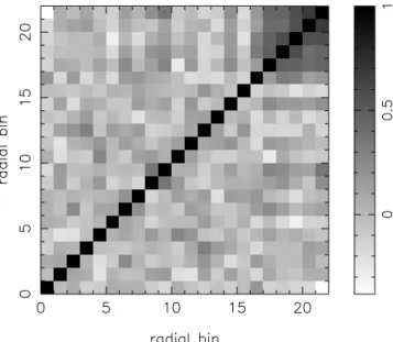
Fig. 6.Normalised covariance matrix between the radial bins of the
lensing measurement and the cluster-satellite correlation for the clus-ters in the N4z1 sample (the fourth richness bin of the first redshift slice, see Table2). The first 11 bins are the radial bins of the lens-ing measurements between 0.15 < r < 5h−1
70 Mpc, the second set of 11 bins are the radial bins of the cluster-satellite correlation be-tween 0.15<r<5h−1
70Mpc.
where
βs=
Dls
Ds
D∞
Dl∞, (9)
withD∞ andDl∞ the angular diameter distance from the ob-server to a source at infinity, and between the lens and a source at infinity. We determine βs and β2s by integrating over
the source redshift distribution, as determined from the pho-tometric redshift catalogues of Ilbert et al. (2013). These re-duced shear models are then fitted to the data. All lensing signals and model shears that we show in the following sections corre-spond to the reduced shear. Note thatβs andΣcritin Eq. (8) are
computed using the mean lens redshift for each cluster sample, rather than integrated over the lens redshift distribution. We have checked that the difference is of the order a few percent, and can be safely ignored.
In short, the model that we fit to the lensing signal is given by ΔΣmod(r) = ΔΣBCG(r)+pcΔΣNFW(r)
+(1−pc)ΔΣmis(r)+ ΔΣ2h, (10)
withpcthe fraction of clusters that is correctly centred. Rather
thanpcwe fitq, defined as pc ≡1/[1+exp(−q)], which has an
infinite range and can therefore be assigned a Gaussian prior. A high value ofqcorresponds to a low miscentring fraction.
2.3.1. Constraining the miscentring distribution
constraints on the miscentring distribution, bypassing the need for using informative priors on the miscentring parameters.
The satellites of a cluster trace the dark matter distribution, although the slope of their radial distribution may differ from the slope of the projected total mass distribution (e.g.Watson et al. 2010,2012;Budzynski et al. 2012;Tal et al. 2012). Here, we use all red-sequence candidates at the cluster redshift brighter than M+1 as satellites. We use this magnitude cut to ensure that our selection is homogeneous and complete over the entire red-shift range of our clusters. We measure their radial distribution by correlating their positions to those of the BCGs. If a frac-tion of the clusters is not correctly centred, this also affects the observed distribution of satellites. The cluster-satellite correla-tion therefore provides addicorrela-tional constraints on the miscentring distribution of BCGs. Note that miscentring has a significantly smaller effect onΣthan onΔΣ, which is illustrated in Fig. 4 in Johnston et al.(2007). However, the signal-to-noise ratio of the cluster-satellite correlation is five to ten times larger than the one from shear, so it still provides useful additional constraints.
We measure the cluster-satellite correlation as follows:
ξcs(r)=n¯rs
Nrs(r)
Nrand(r)×
Nrandtot Ntot
rs
−1
, (11)
with Nrs(r) and Nrand(r) the number of red-sequence galaxies
and random points in a radial bin with a projected radial sep-arationr from the BCG. Ntot
rand and N tot
rs are the total number
of red-sequence galaxies and random points, respectively. The part between brackets measures the overdensity of red-sequence galaxies with respect to their average number density, ¯nrs. We
therefore multiply it with ¯nrs to convert it to the projected
den-sity of red-sequence galaxies in counts per Mpc2. The signal of
the total cluster sample is shown in Fig.5.
To account for zero-point and PSF variations, we scale the number of randoms to the number of red-sequence galaxies in each field separately. Secondly, we determine the ratio of the total number of red-sequence galaxies and the total number of random points in all fields as a function of position in the cam-era, and correct our measurement with this ratio. The purpose of this correction is two-fold. First, it ensures that the random points have exactly the same footprint as the red-sequence galax-ies. Secondly, it accounts for PSF variations across the camera. In particular, the chips in the corners of the mosaic have fewer galaxies, as the average PSF is larger than in the central chips.
To model the cluster-satellite correlation, we assume that the satellites trace the surface mass density of the dark matter, but, motivated by the results fromWatson et al.(2010,2012), Budzynski et al.(2012),Tal et al.(2012) and others, we allow the concentration of the satellites,cgal, to vary. Since we do not
know a priori how the number of satellites is related to the sur-face mass density of the model, we fit this with a nuisance pa-rameter, followingξcs(r)= Agal×Σ(r), withAgal in unitsM−1,
and marginalise over it.
2.3.2. Intrinsic scatter mass-richness relation
The mass-richness relation has intrinsic scatter; therefore, the best-fit lensing mass is not equal to the mean mass of the clus-ters in a bin. To account for this scatter,Johnston et al.(2007) integrate their models over the probability distribution of halo masses,P(M200), given by a log-normal distribution ofM200for
a given N200, and fit the variance in ln(M200). The results of
Becker et al.(2007) andEvrard et al.(2008) are used as a prior on the variance, which are based on a satellite kinematics study of maxBCG clusters and simulations, respectively.
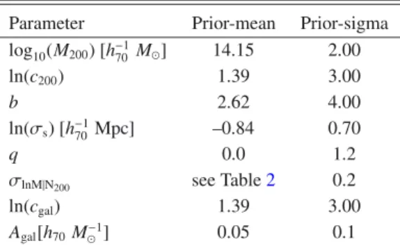
Table 1.Priors on fit parameters.
Parameter Prior-mean Prior-sigma log10(M200) [h−1
70 M] 14.15 2.00
ln(c200) 1.39 3.00
b 2.62 4.00
ln(σs) [h−1
70Mpc] –0.84 0.70
q 0.0 1.2
σlnM|N200 see Table2 0.2
ln(cgal) 1.39 3.00
Agal[h70M−1] 0.05 0.1
More recently, Rozo et al. (2009) studied the scatter in the mass-richness relation using X-ray measurements of the maxBCG clusters, and foundσlnM|N200 = 0.45+
0.20
−0.18 (95%
confi-dence limits). This variance is smaller than the one fromBecker et al.(2007); the difference was likely caused by the fact that Becker et al.(2007) did not account for the miscentring of clus-ters. Therefore, we use the results fromRozo et al. (2009) to account for the scatter.
Since the scatter cannot be constrained by our data, it is im-portant to estimate the prior as accurately as possible. The scatter of the mass-richness relation fromRozo et al.(2009) is com-puted at a fixed richness. Our richness bins span a considerable range, which broadens the actual distribution of halo masses. To obtain a more representative value for the scatter, we take the following approach. We use a mass-richness relation to predict the mass of each cluster in a particular richness bin, and adopt that as the mean of a log-normal probability distribution with a constantσlnM|N200 =0.45. We then combine the probability
dis-tributions of all clusters in that richness bin, and fit a log-normal distribution to it. We adopt the best-fit width as the scatter and list it in Table2. We set the prior width to 0.2, which is the error onσlnM|N200fromRozo et al.(2009).
We use the mass-richness relation from Johnston et al. (2007),M200=8.8×10¹³(N200/20)1.28h−1M. In principle, we could follow an iterative approach where we update the mass-richness relation with our findings, but given that the relation we derive is not very different, and given that the derived scat-ter is fairly insensitive on the adopted relation, we regard this as unnecessary.
2.3.3. Model fitting
To efficiently sample parameter space and fit the models in a rea-sonable amount of time, we use E
mcee
(Foreman-Mackey et al. 2013), the publicly available ensemble Markov chain Monte Carlo (MCMC) sampler. The free parameters in this model areM200,c200,b,σs,q,σlnM|N200,cgalandAgal. For convenience,we summarise the priors in Table1. Note that for all but one parameter,σlnM|N200, the priors are uninformative, hence the
re-sults do not depend on them. We assess how the best-fit masses depend on the prior ofσlnM|N200in the results section.
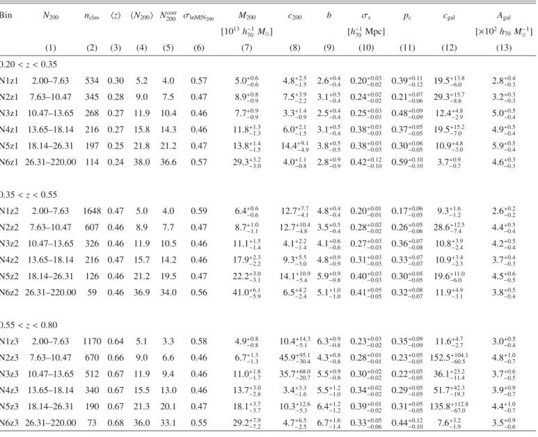
Table 2.Cluster sample details.
Bin N200 nclus z N200 Ncorr200 σlnM|N200 M200 c200 b σs pc cgal Agal
[1013h−1
70 M] [h−
1
70Mpc] [×10
2h 70M−1]
(1) (2) (3) (4) (5) (6) (7) (8) (9) (10) (11) (12) (13)
0.20<z<0.35
N1z1 2.00–7.63 534 0.30 5.2 4.0 0.57 5.0+0.6
−0.6 4.8+ 2.5 −1.5 2.6+
0.4 −0.4 0.20+
0.03 −0.02 0.39+
0.11 −0.12 19.5+
13.8
−6.0 2.8+ 0.4 −0.3 N2z1 7.63–10.47 345 0.28 9.0 7.5 0.47 8.9+0.8
−0.9 7.5+ 3.9 −2.2 3.1+
0.5 −0.4 0.24+
0.02 −0.02 0.21+
0.07 −0.06 29.3+
15.7
−8.6 3.2+ 0.3 −0.3 N3z1 10.47–13.65 268 0.27 11.9 10.4 0.46 7.7+0.9
−0.9 3.3+ 1.4 −0.9 2.5+
0.4 −0.4 0.25+
0.03 −0.03 0.48+
0.09 −0.09 12.4+
4.8
−2.9 5.0+ 0.5 −0.4 N4z1 13.65–18.14 216 0.27 15.8 14.3 0.46 11.8+1.3
−1.3 6.0+ 2.1 −1.5 3.1+
0.5 −0.4 0.38+
0.03 −0.03 0.37+
0.05 −0.05 19.5+
15.2
−7.0 4.9+ 0.5 −0.4 N5z1 18.14–26.31 197 0.25 21.8 21.2 0.47 13.8+1.4
−1.5 14.4+ 9.1 −4.9 3.8+
0.5 −0.5 0.38+
0.03 −0.03 0.30+
0.06 −0.05 10.9+
4.8
−3.0 5.9+ 0.5 −0.4 N6z1 26.31–220.00 114 0.24 38.0 36.6 0.57 29.3+3.2
−3.0 4.0+ 1.1 −0.8 2.8+
0.9 −0.9 0.42+
0.12 −0.10 0.59+
0.10 −0.10 3.7+
0.9
−0.7 4.6+ 0.3 −0.3
0.35<z<0.55
N1z2 2.00–7.63 1648 0.47 5.0 4.0 0.59 6.4+0.6
−0.6 12.7+ 7.7 −4.1 4.8+
0.4 −0.4 0.20+
0.01 −0.01 0.17+
0.06 −0.05 9.3+
1.6
−1.2 2.6+ 0.2 −0.2 N2z2 7.63–10.47 607 0.46 8.9 7.7 0.47 8.7+1.0
−1.1 12.7+ 10.4 −4.8 3.5+
0.5 −0.4 0.28+
0.02 −0.02 0.26+
0.05 −0.06 28.6+
12.5
−7.4 4.4+ 0.5 −0.4 N3z2 10.47–13.65 326 0.46 11.9 10.5 0.46 11.1+1.5
−1.4 4.1+ 2.2 −1.4 4.1+
0.6 −0.6 0.27+
0.03 −0.03 0.36+
0.07 −0.08 10.8+
3.9
−2.4 4.2+ 0.5 −0.4 N4z2 13.65–18.14 216 0.47 15.7 14.2 0.46 17.9+2.3
−2.2 9.3+ 5.5 −3.0 4.8+
0.9 −0.9 0.31+
0.03 −0.03 0.33+
0.07 −0.07 10.9+
3.4
−2.3 3.7+ 0.4 −0.3 N5z2 18.14–26.31 126 0.46 21.2 19.5 0.47 22.2+3.0
−3.1 14.1+ 10.9 −5.4 5.9+
0.9 −0.8 0.40+
0.03 −0.03 0.30+
0.05 −0.05 19.6+
11.0
−6.0 4.5+ 0.6 −0.5 N6z2 26.31–220.00 59 0.46 36.9 34.0 0.56 41.0+6.1
−5.9 6.5+ 4.2 −2.4 5.1+
1.0 −1.0 0.41+
0.05 −0.05 0.32+
0.08 −0.07 11.9+
4.9
−3.1 3.8+ 0.5 −0.4
0.55<z<0.80
N1z3 2.00–7.63 1170 0.64 5.1 3.3 0.58 4.9+0.8
−0.8 10.4+ 14.3 −5.1 6.3+
0.9 −0.8 0.23+
0.03 −0.02 0.35+
0.09 −0.09 11.6+
4.7
−2.7 3.0+ 0.5 −0.4 N2z3 7.63–10.47 670 0.66 9.0 6.6 0.46 6.7+1.3
−1.3 45.9+ 95.1 −30.4 4.3+
0.8 −0.8 0.28+
0.01 −0.01 0.23+
0.05 −0.05 152.5+
104.1
−60.5 4.8+ 1.0 −0.7 N3z3 10.47–13.65 512 0.67 11.9 9.4 0.46 11.0+1.8
−1.7 35.7+ 68.0 −20.7 5.5+
0.9 −0.8 0.30+
0.02 −0.02 0.22+
0.05 −0.05 36.1+
23.2
−11.4 3.7+ 0.6 −0.5 N4z3 13.65–18.14 340 0.67 15.5 13.0 0.46 13.7+3.0
−2.8 3.4+ 3.3 −1.6 5.5+
1.2 −1.0 0.34+
0.02 −0.02 0.29+
0.05 −0.05 51.7+
42.3
−19.3 3.9+ 0.9 −0.7 N5z3 18.14–26.31 190 0.67 21.3 20.1 0.47 18.1+3.7
−3.7 10.3+ 12.6 −5.3 6.4+
1.2 −1.2 0.39+
0.01 −0.02 0.31+
0.05 −0.05 135.8+
112.8
−67.0 4.4+ 1.0 −0.7 N6z3 26.31–220.00 73 0.68 36.0 33.1 0.55 29.2+7.9
−7.2 4.7+ 6.5 −2.5 6.7+
1.6 −1.4 0.33+
0.05 −0.06 0.44+
0.12 −0.10 7.6+
3.2
−1.9 3.5+ 0.9 −0.6
Notes.(1) richness range of the bin; (2) number of clusters; (3) median redshift; (4) mean richness; (5) mean richness corrected for Eddington bias; (6) prior-mean of the scatter in the mass-richness relation; (7) halo mass; (8) concentration; (9) halo bias; (10) miscentring width; (11) centring fraction; (12) concentration of satellite distribution; (13) amplitude of cluster-satellite correlation.
the median and the 68% confidence intervals of the marginalised posterior distributions.
To fit the models to the data, we need to estimate the covari-ance between the data points. We do this by measuring the signal in each of our 145 2×2 deg patches, from which we create a large number of bootstrap realisations. The covariance matrices are estimated from the different realisations. We show a representa-tive normalised covariance matrix for one of our cluster samples in Fig.6. This figure shows that the lensing measurements are not correlated. We therefore set the off-diagonal elements of the lensing signal, and the correlation of the lensing signal with the cluster-satellite correlation, to zero. The cluster-satellite correla-tion itself, however, is correlated at large scales, hence we keep those off-diagonal terms. The inverse of the resulting covariance matrix is used in the fit. To correct for the bias which is intro-duced when a noisy covariance matrix is inverted (Hartlap et al. 2007), we multiply the inverse covariance matrix with a correc-tion factor (Nsample−Ndata −2)/(Nsample−1), where Nsample is
the number of independent samples used in the bootstrap, in our case 145, andNdatais the number of data points, 22.
2.4. Fit results
We divide the clusters in bins of richness and redshift, as detailed in Table2. Although inherently somewhat arbitrary, these ranges were chosen such that they enable us to reliably measure and study potential trends with richness and redshift. The stacked lensing signals are shown in Fig.7and the cluster-satellite cor-relations in Fig.8, together with the best-fit halo models. The errors on the measurements correspond to the square root of the diagonal of the covariance matrix and indicate the 68% confidence intervals. The trends in the data, such as the kink at∼1 h−1
70 Mpc due to the miscentring of clusters, are well
re-produced by the model. We find an average reduced chi-squared value ofχ2
red =1.1 (with 14 d.o.f. per bin), suggesting that the
Fig. 7.Lensing signalΔΣas a function of projected separation from the BCG for the different cluster samples, split in richness (as indicated on top of each column) and redshift (indicated in each panel). The solid black lines indicate the best-fit cluster halo model, simultaneously fitted to the lensing signal and the corresponding cluster-satellite correlation signal in the range 0.15<r<5h−1
70Mpc. The dotted-dotted-dashed grey line shows the contribution from the BCG, the dotted red line the contribution from correctly centred clusters, the dashed green line the contribution from miscentred clusters, and the dotted-dashed blue line the contribution from neighbouring haloes. The dark red, orange and yellow shaded areas correspond to the 1, 2 and 3σmodel uncertainty.
for all bins, we find that the models underpredict the cluster-satellite correlation at scales 1–2h−701 Mpc, exactly the regime that is difficult to model because of the overlap between the one-halo and two-one-halo term.
To illustrate how well the model parameters are constrained, we show the marginalised posteriors of the fit parameters for the N4z1 bin in Fig.9, together with the priors that were used in the fit. OnlyσlnM|N200 cannot be constrained by the data. For the
other parameters, the choice of the prior is not important as they are well constrained. A wrong choice for the prior ofσlnM|N200,
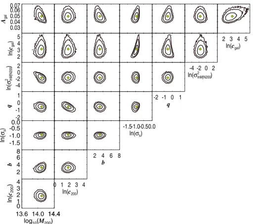
however, could bias our results if degeneracies exist. To investi-gate this, we show the two-dimensional marginalised posteriors of all pairs of parameters in Fig.10.σlnM|N200is only somewhat
degenerate withM200, but not with the other parameters. To
as-sess the sensitivity of our results to the chosen priors, and to en-able a more detailed comparison to the results ofJohnston et al. (2007), we also fit our cluster halo models butonlyto the shear, adopting the priors that were used inJohnston et al.(2007). We discuss how that affects our results in the following section.
3. Mass-richness relation
In order to enable a comparison of our mass-richness relation to simulations, we have to account for Eddington bias: the ob-servational scatter which causes clusters to preferentially move from richness ranges where the abundance of clusters is high to where it is low. This is a separate effect from intrinsic scatter, which defines the width of the halo mass distribution at a given richness if both quantities could be measured with infinite preci-sion, which we account for in our halo model. The observational scatter is mainly caused by the field-to-field variance of the back-ground number density of red-sequence galaxies, for which we use a global estimate. We correctN200for Eddington bias using
Bayes theorem. The probability distribution of the underlying N200given an observed valueN200obs(the posterior) is proportional
to the product of the chance of having a value ofN200obs given a distribution ofN200(likelihood) and the probability distribution
ofN200(prior):
Fig. 8.Cluster-satellite correlation signal, measured using red-sequence candidates brighter than M+1, as a function of projected separation from the BCG, for the different cluster samples, split in richness (as indicated on top of each column) and redshift (indicated in each panel). The solid black lines indicate the best-fit cluster halo models, obtained from simultaneous fits to the lensing signal and the cluster-satellite correlation signal in the range 0.15<r<5h−1
70 Mpc. The dotted red line shows the contribution from correctly centred clusters, the dashed green line the contribution from miscentred clusters, and the dotted-dashed blue line the contribution from neighbouring haloes. Note that the measurements are correlated at large scale (see Fig.5), which is accounted for in the fit. The dark red, orange and yellow shaded areas correspond to the 1, 2 and 3σmodel uncertainty.
The likelihood is determined by the measurement uncertainty ofN200, which our cluster finder provides. The errors are∼20%
larger than Poisson, but we adopt a Poisson distribution as a rea-sonable first order approximation for the likelihood distribution. For the prior, we could in principle use the observed richness distribution. However, as shown in Fig.1, the cluster sample is incomplete at the low richness end by an uncertain amount, and using it as a prior would lead to an erroneous correction. Since we expect that the cluster sample is complete for approxi-matelyN200>15, we fit a power law to the richness distribution
at 20<N200 <40. For the prior, we replace the observed
rich-ness distribution with this power law at N200 < 20, whilst at
larger richnesses we use the observed richness distribution. We sum the posteriors of all clusters in a bin, normalise it and inte-grate up to the mean,Ncorr
200. These values are tabulated in Table2,
as well as the uncorrected values. Only the corrected richnesses are used in the following, unless explicitly mentioned otherwise. We show the mass-richness relation in Fig.11. Note that the mass we show is the mean of the log-normal distribution of halo
masses we integrate over in our halo model. We fit a power-law relation of the formM200 = A(N200corr/20)
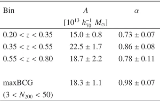
αin each redshift slice and report the best-fit slopes and normalisations in Table3. The errors on the amplitude are determined by marginalising over the slope, and vice versa. The likelihood contours of the fit are shown in Fig. 12. Without the correction for Eddington bias, we would have obtainedA = (14.4±0.7)×1013 h−1
70 Mand
α=0.83±0.08 for the 0.20<z<0.35 bin, which deviates by approximately 1σ.
13.8 14.0 14.2 14.4 log10(M200) 0.00
0.02 0.04 0.06 0.08
0 1 2 3 4
ln(c200) 0.00
0.02 0.04 0.06 0.08
2 4 6 8
b
0.00 0.02 0.04 0.06 0.08
-2.0 -1.5 -1.0 -0.5 ln(σs) 0.00
0.02 0.04 0.06 0.08 0.10 0.12
-2 -1 0 1
q
0.00 0.02 0.04 0.06 0.08
-4 -2 0 2
ln(rlnM|N200
2 )
0.00 0.02 0.04 0.06 0.08
0 1 2 3 4 5
ln(cgal) 0.00
0.01 0.02 0.03 0.04 0.05
0.03 0.04 0.05 0.06 0.07
Agal 0.00
0.01 0.02 0.03 0.04 0.05
Fig. 9.Posteriors of the fitted cluster halo model parameters for the N4z1 bin, marginalised over all other parameters. Black solid lines indicate the
posterior, red lines the prior. The dashed vertical line indicates the median of the marginalised posterior, the blue shaded area is the 68% confidence interval around the median, and the dotted vertical line indicates the location of the best-fit value. Dimensions as in Table2.
13.6 14.0 14.414.4 log10(M200) 0
1 2
3
4
ln(
c200
)
2 4 6 8
b
-1.5 -1.0 -0.50.0
ln(
σs
)
-2 -1 0 1
q
-4 -2 0 2
ln(
σlnM|N200
2
)
2 3 4 5
ln(
cgal
)
0.03 0.04 0.05 0.06 0.07
Agal
0 1 2 3 4 ln(c200)
2 4 6 8 b
-1.5-1.0-0.50.0 ln(σs)
-2 -1 0 1 q
-4 -2 0 2
ln(σlnM|N200
2 )
2 3 4 5 ln(cgal)
Fig. 10.Posteriors of the fitted cluster halo model parameters for the N4z1 bin, for all pairs of parameters. Shown are the 1σ, 2σand 3σconfidence
Fig. 11.Cluster mass versus richness for the cluster samples as indi-cated in the plot. The red circles correspond the results from the lensing analysis of the maxBCG clusters ofJohnston et al.(2007), which have been boosted by a factor 1.18 to account for the impact of photomet-ric redshift scatter (see text). All the measurements that are shown here have been corrected for Eddington bias.
Table 3.Power-law parameters of the fit betweenN200andM200.
Bin A α
[1013h−1 70 M]
0.20<z<0.35 15.0±0.8 0.73±0.07 0.35<z<0.55 22.5±1.7 0.86±0.08
0.55<z<0.80 18.7±2.2 0.78±0.11
maxBCG 18.3±1.1 0.98±0.07 (3<N200<50)
ways, and particular choices can reduce this bias (Mandelbaum et al. 2010). More detailed numerical simulations are required to quantify this bias more precisely, e.g. as a function of mass and redshift, to interpret the results correctly. This is important for the exploitation of clusters as a reliable tool for cosmology.
3.1. Comparison to previous single-redshift results
We compare our results to the weak lensing analysis of the maxBCG cluster sample (Koester et al. 2007), a catalogue of 13 823 clusters that has been detected in the SDSS. The clus-ter detection algorithm employed inKoester et al.(2007) iden-tifies the cluster red-sequence galaxies, and selects the bright-est, the BCG, as centre of the cluster. The resulting cluster sample covers the richness range 10 < N200 < 190 and a
redshift range of 0.1<z<0.3. In Sheldon et al. (2009), the cluster sample is extended to N200 = 3, which leads to a
sample of ∼130 000 galaxy groups and clusters. The lensing analysis of the sample is presented in Sheldon et al. (2009); the mass-richness relation is derived inJohnston et al.(2007).
Fig. 12.67.8%, 95.4% and 99.7% confidence limits of the fits to the
mass-richness relation. The black dotted lines show the results from Johnston et al.(2007) in the overlapping richness range.
FollowingMandelbaum et al.(2008b), we multiply the masses fromJohnston et al. (2007) by a factor 1.18 to account for the impact of photometric redshift scatter in the lensing analysis (as was done inRozo et al. 2010). Note thatJohnston et al.(2007) use the same definition of mass as we do.
The richnesses ofJohnston et al.(2007) have not been cor-rected for Eddington bias. We perform the correction, using a probability distribution for the maxBCG sample of p(N200) ∝
(N200)−3 over the entire richness range, followingAndreon &
Hurn(2010), which is in good agreement with a slope of−3.06 that we find for our clusters with 0.2<z<0.35 andN200>15.
We adopt the mean richness asNobs
200to compute the posterior,
in-stead of stacking the posteriors of the individual clusters. This makes a negligible difference. We show the corrected results in Fig.11. We fit the same power law in the overlapping rich-ness range, 3 < Ncorr
200 < 50, and list the best-fit parameters in
Table3. The amplitude and slope of our low-redshift sample are about 3σlower than those of the maxBCG. Figure11shows that this discrepancy is partly driven by the bins atN200 <10. If we
fit the relation at N200 > 10, the slopes are consistent but the
amplitudes still differ by∼2.5σ.
There are several differences between the analyses. For in-stance, Fig.4suggests that our richnesses are somewhat larger than those of the maxBCG for rich systems; how they differ at low N200 is unclear as the public maxBCG catalogue only
in-cludesN200 > 10 clusters. If our richnesses are systematically
N200 > 10; how the purity varies at lower richnesses is not
re-ported. Since the purity of the RCS2 cluster sample is expected to be high as well, it seems unlikely that differences in the purity could lead to differences larger than a few percent in the masses. Also on the modelling side, there are noticeable differences. For example, we use different priors for the miscentring distri-bution and for the scatter between richness and halo mass. In Johnston et al.(2007), the miscentring priors are based on nu-merical simulations, from which a functional form is derived forq, with a corresponding pc (the fraction of clusters that is
correctly centred) ranging from 60% to 80% for richnesses in the range ofN200 = 10 toN200 = 100. The width of the
mis-centring distribution is fixed at 0.42h−1 Mpc. Our best-fit pa-rameter suggest a pc in the range of 20–50%, and a narrower
widthσs ≈0.2−0.4h−701Mpc. It is conceivable that the
miscen-tring distribution differs for the two catalogues, as different algo-rithms have been applied to different data to identify the BCG. However, if the actual miscentring distributions are similar, the different priors could cause discrepancies between the best-fit masses and concentrations due to the parameter degeneracies. The same holds for the adopted prior for the scatter in mass-richness. Motivated by this, we run our cluster halo models on the lensing data only, using the priors fromJohnston et al. (2007). Note that we do not account for the differences between the two-halo terms. Nevertheless, this test will give us a rea-sonable impression how sensitive our results are to the adopted priors.
The resulting best-fit masses of the individual bins are con-sistently lower but within the 1σerror bars of the nominal re-sults. When we refit the power-law relation, we find an amplitude and slope ofA=(12.2±1.2)×1013h−1
70 Mandα=0.69±0.15
for the 0.20 <z <0.35 redshift slice, which is even more dis-crepant. Comparing this to our nominal results shows that the tighter constraints on the miscentring distribution, obtained from including the cluster-satellite correlation in the fit, also leads to smaller errors on the mass. As the amplitude is∼2σlower than our nominal result and the slope is consistent, our results do not critically depend on the adopted priors. Furthermore, we have also checked that by changing the implementation of the two-halo term, the masses do not change significantly.
The mass-richness relation has also been derived from semi-analytic galaxy formation models based onN-body simulations. For example, Hilbert & White (2010) used the Millennium Simulation (Springel 2005) and found that the derived mass-richness relation agreed well in shape and amplitude with the relation from maxBCG.Hilbert & White(2010) report an am-plitude and slope of A = (17.7 ±0.1)×1013 h−1
70 M and
α=1.09±0.01. The amplitude and slope are a bit higher than our low-redshift results. The difference is again mainly driven by theN200 <10 results, but additionally, some difference may
be caused by the different definitions of richness.Angulo et al. (2012) measure the relation between optical richness and mass atz =0.25 in the Millennium-XXL simulation, which extends the Millennium and Millennium-II Simulations (Springel 2005; Boylan-Kolchin et al. 2009). A power-law slope of 1.07 is re-ported, steeper than our results, but again the difference may originate from the low-richness end and from differences be-tween the richness estimators.
InFord et al.(2015), a sample of 18 000 optically selected clusters at 0.2 < z < 0.9 are studied in the Canada-France-Hawai Telescope Lensing Survey (CFHTLenS;Heymans et al. 2012). Clusters are identified using the 3D-Matched-Filter finder ofMilkeraitis et al.(2010). Richnesses are defined as all cluster members withinr200 that are brighter than an absolute i-band
magnitude of−19.35, as detailed inFord et al.(2014). It is not clear how that relates to our richness estimate. Using the same parametrisation of the mass-richness relation as we do, they find an amplitude and slope of 2.7+0.5
−0.4×10¹³Mand 1.4±0.1,
respec-tively. No correction for the Eddington bias is performed, lead-ing to a larger slope. However, the normalisation is significantly lower than what we find. The difference may be partly attributed to the definition of richness (see the discussion in Sect. 5.3 of Ford et al. 2015).
3.2. Redshift evolution
At any given richness, clusters at 0.35<z<0.55 have larger masses than those at 0.2 < z < 0.35. Whether this trend con-tinues towards higher redshifts is not clear given the large errors on the mass for the 0.55<z<0.8 clusters, although our results suggest that it does not.
Both the halo masses and the richnesses of clusters may evolve. The bulk of the change in halo mass is not expected to be physical accretion, but rather an effect called pseudo evolu-tion (Diemer et al. 2013). Halo masses are defined with respect to a background density (usually the mean or the critical den-sity), which evolves with redshift. Even if a halo does not accrete anything, its mass increases with time as the background density drops. If the richness of a cluster would not change, we would expect to see an increase in halo mass towards lower redshifts. The fact that we find the opposite trend and that the halo mass decreases at a given richness, points towards an evolution of the richness.
Clusters build up their red sequence over cosmic time. The cluster galaxies are stripped of their gas through tidal in-teractions and ram pressure stripping, which quenches their star formation (e.g. Boselli & Gavazzi 2006). Consequently, the late-type spiral galaxies that are accreted turn into early-type S0 galaxies, and subsequently appear on the E/S0 ridge line. Hence even without accreting new galaxies,N200, the
red-sequence richness, increases as more galaxies turn red. Various works have reported an increase of the number density of faint red-sequence cluster members toward low redshift (e.g. Loh et al. 2008;Gilbank et al. 2008;Rudnick et al. 2009;Jaffé et al. 2011;Vulcani et al. 2011). For example,Rudnick et al.(2009) measure the optical cluster luminosity function of red-sequence galaxies at z < 0.8. They find that at magnitudes brighter thanM, the luminosity function does not evolve much, suggest-ing that these cluster members are already in place. However, at fainter magnitudes, the luminosity function strongly increases towards lower redshift. This supports the view that cluster rich-nesses (defined with aM+1 magnitude limit, as we do) may become larger towards lower redshift, in line with what our re-sults suggest. There may be other processes that could cause an evolution ofN200. Mass segregation could lead to more bright
cluster members within the inner one Mpc, which would boost Ngal, leading to higher values forrgal200andN200. Mergers of
clus-ter members both brighclus-ter than M +1 would lower N200, but
mergers of faint red-sequence members could increase it. The build-up of the red sequence, however, is likely the dominant effect.
Fig. 13.Cluster mass versus the width of the miscentring distribution (top), versus the width divided byr200(middle) and versus the fraction of “correctly centred” BCGs, the ones that are located at the centre of the halo (bottom). The black dashed lines show the fitted relation be-tween miscentring parameter and mass, as described in the text.
is twice as high as the X-ray luminosity atz=0.14.Becker et al. (2007) studied the relation between velocity dispersion and rich-ness for the same clusters, and found that the clusters at high redshifts systematically have higher velocity dispersions. Both Becker et al.(2007) andRykoffet al.(2008) expected the main cause to be the evolution of theN200 richness measure,
imply-ing a fractional decrease inN200of 30–40% fromz = 0.14 to
z=0.28. We ignored this effect when we compared our results in Fig.11, but since the mean redshift of maxBCG clusters is 0.25, very close to the mean redshift of our low-redshift clusters, it is not important. If we ignore the potential evolution in halo mass, our results suggest a fractional decrease of 34±4% inN200from
z=0.27 toz=0.46.
Andreon & Congdon(2014) measure the richness and mass for a sample of 23 very massive clusters with 0.15<z<0.55 within a fixed aperture of 0.5 Mpc. This “aperture” mass-richness relation does not evolve with redshift. Most of the ac-cretion and quenching of new cluster members happens at the outskirts of galaxy clusters (e.g.van der Burg et al. 2015), and may be missed when using an 0.5 Mpc aperture. Furthermore, the selection of red cluster galaxies and the computation of rich-ness differ from our work, which may contribute to the apparent discrepancy between the results.
4. Miscentring distribution
By fitting the shear measurements together with the cluster-satellite correlation, we obtain, for the first time, tight constraints on the miscentring distribution of BCGs with respect to the cen-tre of their dark matter haloes. Figure13shows that∼30% of our BCGs are located at the centre of the halo. The distribution of the miscentred BCGs is described by a 2D-Gaussian with a standard deviation that increases from∼0.2 to∼0.4h−1
70 Mpc going from
our poorest to our richest clusters; the ratio of width andr200is
flat with mass. Since the miscentring parameters do not appear to evolve with redshift, we combine all our cluster samples and parametrise the relations as pc=Ap+Bp×(log10(M200)−14),
obtaining Ap = 0.29 ± 0.02 and Bp = 0.16 ± 0.07,
andσs =Aσ+Bσ×(log10(M200)−14), finding Aσ = 0.29±
0.01 [h−1
70 Mpc] andBσ=0.31±0.03 [h70−1Mpc/log10(h−701M)].
Since cluster members are spread over a larger volume in more massive clusters, we expect that the mass dependency is re-duced when we consider the ratioσs/r200. Indeed we find this
ratio is consistent with a constant, for which we obtain a value of 0.44±0.01 for all samples combined. The average for the low-, intermediate- and high-redshift slices are 0.42 ± 0.02, 0.40±0.02 and 0.51±0.02, respectively. Note that we account for the errors on both the dependent and independent parame-ters in the fit. The high-redshift slice has an intrinsically broader miscentring distribution, which may reflect that more clusters are still undergoing mergers at that redshift, or that the BCG is more often misidentified due to increased photometric errors. This miscentring distribution is different from the one adopted inJohnston et al.(2007), which was based on mock catalogues determined from simulations that were fit to a range of obser-vations. There, a much higher fraction of 60–80% of the BCGs was found to be correctly centred. The width of the miscentring distribution was found to be 0.42h−1Mpc, larger than what we
find. The lensing signal itself cannot discriminate between their miscentring distribution and ours, but the cluster-satellite corre-lation is able to break the degeneracy.
It is possible that the difference between the miscentring dis-tributions is the result of the different algorithms used to identify the BCG. This could be tested by applying both algorithms to the same set of simulations or data. However, part of the discrepancy could also be due to how the simulations used inJohnston et al. (2007) are constructed. In these simulations, every dark matter halo is assumed to have a BCG at its centre. Hence misidenti-fying the BCG is the only reason why the centring fraction is less than 100%. However, in reality, the central BCG may ac-tually be displaced by a small amount from the centre of the halo. This would push the centring fraction down and lower the width of the miscentring distribution, more in line with our find-ings. Also, some BCGs may be star forming, leading to too blue colours to be selected as red-sequence member (Bildfell et al. 2008).
The location of BCGs in clusters has been studied in vari-ous other works.Skibba et al.(2011) study mock catalogues and SDSS group catalogues and report that in 40% of their groups with a mass larger than 5×10¹³ h−1M
, the brightest galaxy is a satellite galaxy instead of the central galaxy. Using N-body simulations, Martel et al. (2014) find that the fraction where the brightest galaxy is not the nearest to the centre increases from ∼25% to ∼50%, with a higher miscentring fraction to-wards higher mass.Hoshino et al.(2015) study the distribution of LRGs in the redMaPPer clusters (Rykoffet al. 2014) and find that 20–30% of the brightest LRGs are not the central galaxy. As the central galaxy might be somewhat offset from the peak of the dark matter, these results might be in agreement with our results. Remarkably, bothSkibba et al.(2011) andMartel et al. (2014) find that the centring fraction actually decreases with in-creasing mass, in contrast to what is assumed inJohnston et al. (2007). This is attributed inMartel et al.(2014) to cluster merg-ers, which have occurred most recently in more massive clusters as they are the last ones to form. Our centring fractions do not show a clear trend with mass.