Software Tools and Guide for Viscoelastic Creep Experiments
Jessica Wehner
A thesis submitted to the faculty of the University of North Carolina at Chapel Hill in par-tial fulfillment of the requirements for the degree of Master of Science in the Department of Mathematics.
Chapel Hill 2010
Approved by:
M. Gregory Forest
Laura Miller
Abstract
JESSICA WEHNER: Software Tools and Guide for Viscoelastic Creep Experiments. (Under the direction of M. Gregory Forest.)
Models predicting strain as a function of time are fit to data obtained from creep recovery
experiments on viscoelastic materials. Here we discuss standard non-inertial and
instrument-induced inertial creep experiments. We first summarize and illustrate key signatures, which
differentiate the models and highlight properties of creep data. The basic signatures
distin-guishing a solid versus fluid response, respectively, are: a sudden versus gradual rise when
a stress impulse is applied; a sudden versus gradual decline when a constant stress is
sud-denly removed; and recovery to zero strain versus a finite steady state after the applied stress
is removed. For completeness, we discuss development of the models, solution methods, and
parameter influence on behavior. Finally, software created by Dr. Ke Xu to estimate the model
parameters that best fit the experimental data is adapted to illustrate the influence of
Table of Contents
List of Figures v
1 Experimental Rheology 1
1.1 Overview of Creep Experiments . . . 1
1.2 Mechanical Models . . . 5
1.3 Illustration of Experimental Data . . . 8
2 Non-Inertial Models 12
2.1 Overview of Non-Inertial Models . . . 13
2.2 Example: Derivation of Analytical Solution to Three Parameter Maxwell Model 15
2.3 Linear Viscoelastic Liquid Models . . . 17
2.4 Linear Viscoelastic Solid Models . . . 21
2.5 Summary of Model Signatures of Non-Inertial Creep Experiments . . . 25
3 Inertial Models 27
3.1 Overview of Inertial Models . . . 27
3.2 Example: Coupling of Instrumental Inertia to Maxwell Model and Derivation
of Analytical Solution . . . 28
3.3 List of Inertial Models . . . 33
3.4 Summary of Model Signatures of Inertial Creep Experiments . . . 36
4 Software Tools 38
4.1 Parameter Inference and Analysis of Parameters Using Mathematica . . . 39
4.2 Generating Experimental Error: Make Data Tool . . . 45
4.3 Experimental Parameter Fittings after Identification of Key Signatures . . . 53
List of Figures
1.1 Schematic of cone and plate rheometer . . . 2
1.2 Response of a pure solid and liquid . . . 4
1.3 The viscous element represented as a dashpot . . . 5
1.4 The elastic element represented as a spring . . . 5
1.5 Two Parameter Maxwell element . . . 6
1.6 Three Parameter Maxwell element . . . 7
1.7 Agarose under high stress . . . 9
1.8 Highly oscillatory agarose data appears noisy . . . 10
2.1 Top hat stress function . . . 14
2.2 Two Parameter Maxwell model . . . 19
2.3 Maxwell-Jeffrey model . . . 20
2.4 Three Parameter Maxwell model . . . 22
2.5 Two Parameter Kelvin-Voigt model . . . 23
2.6 Three Parameter Kelvin-Voigt model . . . 24
3.1 Inertial Maxwell model . . . 33
3.2 Inertial Voigt model . . . 34
3.3 Inertial Maxwell-Jeffrey model . . . 35
4.1 Screen shot of Mathematica ‘manipulate’ tool . . . 40
4.2 Comparing changes in small G for smallηin 3 Par. Voigt . . . 42
4.3 Comparing changes in large G for smallηin 3 Par. Voigt . . . 42
4.4 Observing the effects ofη2on slope in Maxwell-Jeffrey . . . 44
4.5 Parameter values for Maxwell-Jeffrey across range of error . . . 45
4.6 Effects ofη2on fitting region(0,5) . . . 46
4.7 Good alignment on fitting interval . . . 46
4.8 Comparing original data to graph generated by poorly fit parameters . . . 47
4.9 Make Data environment . . . 48
4.10 Close up of ‘Parameter Values’ box in make data.fig . . . 48
4.11 Close up of ‘Set Details of Applied Stress Function’ box in make data.fig . . . 49
4.12 Close up of ‘Options’ box in make data.fig . . . 49
4.13 Demonstration of fitting algorithm on data with 5% error . . . 51
4.14 Summary of controls tested to examine influences of experimental error . . . . 51
4.15 Error in predictions ofGandηfor different levels of experimental error . . . . 52
4.16 Experimental data resembling Three Parameter Maxwell or Voigt models . . . 53
4.17 A poor versus good fit in experimental data . . . 55
4.18 Agarose data at 0.05 Pascals . . . 56
4.19 Agarose at 0.05 Pascals fit to Linear Solid and Maxwell-Jeffrey . . . 57
4.20 Agarose data at 0.2 Pascals . . . 58
4.21 Agarose at 0.2 Pascals fit to Linear Solid and Maxwell-Jeffrey . . . 59
4.22 Agarose data at 0.5 Pascals . . . 60
4.23 Agarose at 0.5 Pascals fit to Linear Solid and Maxwell-Jeffrey . . . 61
4.24 Excellent fit to exact inertial data . . . 62
4.25 Poor fit of experimental inertial data on interval(0,5) . . . 63
Chapter 1
Experimental Rheology
1.1 Overview of Creep Experiments
One tool for exploring the properties of viscoelastic materials is the creep experiment.
Typ-ically, a shear stress (force per unit area, given here as τ) is imposed on the material in a prescribed manner (with a known magnitude usually measured in pascals and with dictated on
and off times) by a rheometer. The sample is trapped between two small plates in the
rheome-ter, and shear stress is applied to the fluid through the controlled torque rotation of the top plate
relative to the bottom. The top and bottom plate can both be flat and parallel, as in a parallel
plate rheometer; or the top plate can be an inverted cone with a very shallow angle, as in the
cone and plate rheometer. A controlled torque is imparted to the top plate, and its angular
deflection is measured with high accuracy as it rotates with influence from the thin layer of
material beneath it. From this we can take measurements of how the sample deforms under the
applied stress and how it recovers once the imposed stress is removed.
The geometry of a cone and plate rheometer is depicted below in Figure 1.1. The values
(Macosko94) for further details.
Figure 1.1: Geometry of a cone and plate rheometer with diameterR, cone angleβand angular deflectionφ.
Under constant stress as in these experiments, the linear response of a viscoelastic material
is proportional to the imposed stress. (This will be evident below when we give the model
equations and their closed-form solutions.) Thus, it is natural to normalize strain by the
im-posed stress. This defines the compliance,J=γ/τ. In this manner, the material responseJ is independent of the value of the input stress. A good experimental test of linear response is to
run the experiment at several stress levels. All the data should collapse onto a single curve,
the compliance curve. The mathematical models used here, which predict strain values, are
converted to compliance before use with compliance data.
By plotting the compliance as a function of time, we can obtain graphs with standard
fea-tures which are unique for different types of materials. An overarching goal is to find
math-ematical models which best reflect these features, to which end there are many standard
me-chanical models used in practice which will be discussed in this document. Additionally, two
types of creep experiments can be performed and each may collect unique information. These
are the inertial and non-inertial experiments.
Performing an inertial experiment means that the inertia of the rotating parts of the
rheome-ter is allowed to enhance the elasticity of the marheome-terial resulting in oscillatory behavior in the
response, sometimes referred to as ‘ringing’. Initially, only non-inertial experiments were
in-terference with the data. However, a very small amount of oscillatory behavior present at the
beginning of these experiments could be noted. These first few moments would be removed
from the data to prevent it from interfering with further analysis. It was then discovered, as
noted in (Barav98), that the inertia of the instrument could be coupled to the material’s
elastic-ity to aid in the study of thixotropy. Thixotropy can be described as the time dependent change
in viscosity that a material might undergo during a stress experiment. Although we are not
concerned with how to model thixotropy in this thesis, we will provide evidence while fitting
to experimental data that thixotropy occurs in certain materials. It is important to consider
the coupling of instrumental inertia for other reasons than to study thixotropy; these include a
much shorter timescale on which useful information may be collected and the ability to infer
more information from a single experiment.
Material behavior
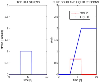
For a simple elastic response, the governing equation is Hooke’s law: stress (τ) is proportional to strain (γ) with the shear modulus (G) as the constant of proportionality,τ=Gγ. The simplest equation to describe a purely viscous response is Stokes relation: stress (τ) is proportional to rate of strain (˙γ) with constant of proportionality the viscosity (η), τ=ηγ˙. Both of these models have been around since the 1660s. Let’s observe how these simple equations respond
to an imposed constant stress that is turned on att0 and turned off att1 (this is equivalent to a
top hat function which can be written asτ=H(t−t0)−H(t−t1)).
Hooke’s law can be solved directly forγ,γ=Gτ. Thus, the strain of a pure solid will mimic the top hat function but with a changed magnitude dependent on G. At the onset of stress,
the solid will suddenly reach some constant strain, maintain that strain for the duration of the
applied stress, and then suddenly recover to its resting configuration (recover fully to 0 strain).
This is a result of a solid’s ability to store stress as it is applied and release it once stress is
removed. As another example, if the stress is sinusoidal instead of top hat, the response of an
elastic material will remain in phase with the stress. Just considerτ=sin(t)and observe that
γ= G1sin(t)has a new amplitude but remains in phase.
Solving Stoke’s Law for γ requires an integration of the applied stress; in this case, the integration of two step functions results in two linear functions. The result isγ=η1[(t−t0)H(t−
t)−(t−t1)H(t−t1)]. This and the elastic response above are depicted in Figure 1.2. At the
onset of stress, the pure liquid will strain linearly. Once the stress is removed, the liquid will
maintain the acquired configuration and will not recover any strain. This is because a purely
viscous material cannot store stress and hence deforms continuously as shear stress is applied.
The strain of a fluid will beπ/2 radians out of phase with a stress that is applied sinusoidally. For example, ifτ=sin(t), thenγwill be given by a cosine function, which isπ/2 radians out of phase with sine.
0 5 10 0
0.5 1 1.5 2 2.5 3
time [s]
stress [Pascals]
TOP HAT STRESS
0 5 10 0
0.5 1 1.5 2 2.5 3
time [s]
strain
PURE SOLID AND LIQUID RESPONSES SOLID
LIQUID
Figure 1.2: The response of a pure solid (red) and a pure liquid (blue) to an applied top hat stress.
Viscoelastic materials exhibit both viscous and elastic properties, yet can be more
solid-like or liquid-solid-like in their response to constant or phasic shear stress. Thus, an initial focus
solid-like at the applied stress level. A further complicating observation is that many viscoelastic
materials are solid-like at sufficiently low stress levels, yet liquid-like above a stress threshold.
This thesis will only give an example of such materials, but the tools presented here can detect
such behavior simply by varying stress levels in a series of creep experiments across the critical
threshold.
It should be noted that the most general distinction of ‘liquid-like’ or ‘solid-like’ used
to categorize the models in Chapter 2 is chosen here based on end behavior - if the model
recovers to 0 strain after stress is turned off, it is denoted as a linear viscoelastic solid; if the
model recovers to some positive steady state strain when stress is turned off, it is denoted as a
linear viscoelastic liquid. The other features considered here, such as an initial jump in strain
at the onset of an applied stress or a sudden drop in strain once stress is removed, can also be
considered liquid-like or solid like. However, because of our choice to use end behavior as the
broadest category, the other features will be intermixed between solid- and liquid-like models.
1.2 Mechanical Models
The basic viscous and elastic elements can be represented as mechanical forms having a
gov-erning constitutive law. The basic viscous element is represented as a dashpot. As its purpose
is to represent a purely viscous response, it is governed by Stokes relation described above:
τ=ηγ˙. The basic elastic element, meant to represent a purely elastic response, is represented as a spring and is governed by Hooke’s law:τ=Gγ. See Figures 1.3 and 1.4.
Figure 1.3: The viscous element repre-sented as a dashpot, with viscosityη.
Figure 1.4: The elastic element repre-sented as a spring with shear modulusG.
To build a viscoelastic material, the spring and dashpot elements can be combined in series
and parallel configurations, achieving new behavior with at least two parameters - G and η. Certain rules define how the governing equations are combined. These configurations and their
equations have given rise to the several standard linear viscoelastic models used today and are
presented in detail in further sections of this document. However, to give a thorough example
of how one such model might be developed, we shall now go through the steps which lead
to the standard Three Parameter Maxwell model. All other models are developed in the same
manner; an excellent reference for all of these models is (Tschoegl89).
Deriving the Three Parameter Maxwell model
The Three Parameter Maxwell mechanical model is created by combining a Maxwell element
in parallel with a spring. Thus, first we must know how to create the Maxwell element. The
Maxwell element is the series combination of one spring and one dashpot, as shown below.
The rule for series configurations is that the strains add and the stresses are distributed equally.
Figure 1.5: Two Parameter Maxwell element
For the dashpot (viscous element) we haveτv=η˙γv. For the spring (elastic element) we have
τe=Gγe. Adding strains means that the overall strain of the two parameter model is the sum of the strains of each element,γ=γe+γv. Thus,
˙
γ = γ˙e+γ˙v = τ˙e
G+
τv η
Since equating stresses means thatτ=τe=τv, we can substituteτ, the overall stress of the
two parameter model, forτe andτv, the stresses of the individual elastic and viscous elements,
respectively. Thus, we have ˙γ= G˙τ +ητ. We can divide through byηto get as the constitutive law of the two parameter Maxwell element the equationηγ˙= Gητ˙+τ, which we note is trivial to solve forγ/τ0by one integration.
To create the Three Parameter Maxwell model we combine the Maxwell element in parallel
with a spring, as shown below. Now, the law which governs the maxwell element was found
Figure 1.6: Three Parameter Maxwell element
to be η1γ˙1= Gη11τ˙1+τ1, and the law which governs the spring is given by τ2=G2γ2 (using
subscripts to differentiate between parameters). We wish to combine these two elements (the
spring and the maxwell) in parallel, for which the rule is to add stresses and distribute strains
equally. Thus, noting that ˙τ1=τ˙−τ˙2=τ˙−G2˙γ, we have
τ = τ1+τ2
=
µ
η1γ˙1− η1
G1τ˙1
+G2γ2
= η1˙γ−η1
G1τ˙1+G2γ
= η1˙γ−η1
G1(
˙
τ−G2γ) +˙ G2γ
(1.2)
From here we can simplify, obtaining
˙
τ+G1
η1τ= (G1+G2)˙γ+
G1
η1G2γ (1.3)
as the constitutive law for the Three Parameter Maxwell model.
1.3 Illustration of Experimental Data
The data used here are the same as in (Xu2009), for which she describes the preparation as
follows:
... low melting point agarose (Sigma product number A9414) is mixed to 0.3% in the same buffer (0.2M NaCl, 0.01EDTA, and 0.01% Sodium Azide). The sam-ples’ rheological properties are determined by a Bohlin Gemini Rheometer in both cone and plate ( 60mm diameter, 1 degree, 7.9103mm3 in volume) and parallel plate (20mm diameter, 50um gap, 63mm3 in volume) geometries under the stress amplitude sweep mode.
In order to illustrate the models, exact data generated directly from each model will be used.
However, in reality experimental data is not always ‘clean’ and therefore cannot be expected
to match perfectly any one model. For example, creep experiments are best done at low stress
levels. With too high stress (above the stress threshold), the results are compromised and
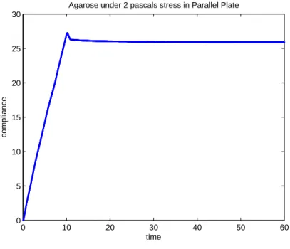
informative features cannot be extracted. Consider Figure 1.7 showing agarose data at a stress
of 2 pascals. The compliance has no curvature - it essentially ramps up continuously until the
stress is removed at 10 seconds, at which point it relaxes to a high value and remains there,
similar to a pure liquid. The stress was high enough to ‘overpower’ the elasticity in the sample,
and any stress at this level or higher will be unable to capture the viscoelastic properties of the
material.
Experimental error is also always present in the data. Generally it is easy to see what
the features of the graph are despite the error. Because it is random error we are capable of
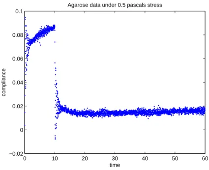
ignoring unusually extreme values and inferring what the curve ‘should’ look like. The data in
Figure 1.8 looks like it could be very noisy data. In actuality, most of the ‘noise’ is rather high
frequency oscillations that are not apparent under this scaling. However, in the later parts of the
0 10 20 30 40 50 60 0
5 10 15 20 25 30
time
compliance
Agarose under 2 pascals stress in Parallel Plate
Figure 1.7: When experiments are performed on agarose under too high of a stress, the stress threshold is passed and the material resembles a pure liquid rather than a viscoelastic fluid.
small amount of noise present while viewing a small range. (i.e., if the data were plotted with a
larger range, the experimental error would be relatively smaller and the data would appear less
noisy.) One should also keep in mind that experimental data is discrete. In the data considered
here, time steps of .02 seconds are used. If the frequency of inertial data is higher than the
sampling frequency, then we will be unable to detect oscillations and the data could instead
just appear noisy.
A note on parameter values
The properties of purely viscous and elastic materials are consistent regardless of the type of
stress imposed on them. On the contrary, viscoelastic materials would be expected to behave
much differently depending on the way they are being stressed, say for a sinusoidal stress of
low versus high frequency. It is for this reason that different types of experiments are important
and necessary for probing many different realms of linear viscoelastic responses. It is also
0 10 20 30 40 50 60 −0.02
0 0.02 0.04 0.06 0.08 0.1
time
compliance
Agarose data under 0.5 pascals stress
Figure 1.8: Highly oscillatory agarose data appears noisy.
because of this that it is impossible to identify single parameter values which best describe any
given viscoelastic material. At best, a range of values must be given to describe a range of
driving forces. These ranges can be quite large. Experimentally, the added difficulty is that the
prepared samples cannot be perfectly the same, resulting in a range of recorded experimental
parameters.
Regardless of the fact that the true state of the material varies greatly, our methods for
ex-tracting parameter guesses can also fluctuate. In the context discussed here, statistical
regres-sion is performed on sample data to determine the best fit parameters. Should this regresregres-sion be
performed on the entire data set, or on smaller pieces of the data? If so, how small, and which
pieces? It is important to decide ahead of time, because parameters inferred from different
sections of the same data can report largely different numbers (evidence of nonlinear behavior,
examined further in Chapter 4). As an example, consider this summary of results obtained by
making multiple fits on two data sets. One data set is from an inertial creep experiment on
0.2% agarose at a 0.5 Pascal stress level. The Inertial Maxwell-Jeffrey and Inertial
Kelvin-Voigt models were fit to these data sets at time intervals[0,1],[0,4]and[0,10]. From the table below we can see thatη1seems to have the largest range, in one case ranging from 59 to 464,
while the parameterGremains very consistent across each model on the same data set. More
will be discussed on the sensitivity of parameters in Chapter 4.
0.3% Agarose
Fit for Inertial Maxwell-Jeffrey
η1 G η2 α
[0,1] 59.43 17.978 0.163 0.044
[0,4] 230.11 15.795 0.176 0.038
[0,10] 463.16 14.731 0.183 0.036
Fit for Inertial Kelvin-Voigt
η G α
[0,1] 0.194 15.616 0.038
[0,4] 0.191 13.879 0.033
[0,10] 0.206 12.703 0.030 0.2% Agarose
Fit for Inertial Maxwell-Jeffrey
η1 G η2 α
[0,1] 7.297 2.526 0.074 0.048
[0,4] 37.290 2.152 0.095 0.041
[0,10] 103.779 2.001 0.100 0.038
Fit for Inertial Kelvin-Voigt
η G α
[0,1] 0.124 2.135 0.042
[0,4] 0.104 1.923 0.036
[0,10] 0.109 1.823 0.034
Chapter 2
Non-Inertial Models
2.1 Overview of Non-Inertial Models
In a creep experiment without inertia, stress is applied to the material by a rheometer. A
constant applied stress can be turned on and left on (step stress), turned off after an interval of
time (top hat stress), or applied as a train of pulses. Only step and top hat stress experiments are
considered in this thesis. The material responds to the stress by deforming, and the resulting
displacement is measured and converted to strain (or compliance), which is plotted against time
to produce a strain response curve. The inertia of the instrument is able to be damped to a high
degree to keep from interfering with the strain measurements.
Different characteristics in the responses can then potentially be captured by one of
sev-eral standard models: the Two Parameter Maxwell, Three Parameter Maxwell, Two Parameter
Kelvin-Voigt, Three Parameter Kelvin-Voigt or the Maxwell-Jeffrey. Each is a mechanical
model corresponding to a linear differential constitutive law. The continued usage of these
models has historical precedence coming from the convenience of their ability to be solved in
closed form and their ability to capture key creep features of simple viscoelastic liquids and
solids (whose distinction we emphasize below). In Section 2.3, each model is categorized as a
linear viscoelastic liquid or solid model and is given along with its constitutive law. Solutions
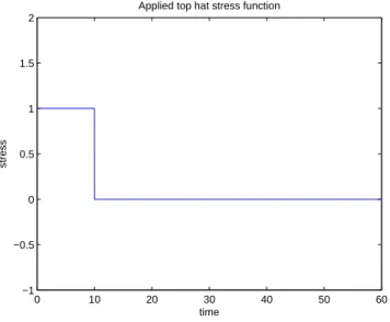
and turned off at timet1. The imposed form of stress used for obtaining the given solutions is
τ(t) =τ0(H(t−t0)−H(t−t1)), where
H(t−x) =
0 ift<x;
1 ift≥x;
is the step function. (Solutions for step stress are found by ignoring the terms containingt−t1,
or equivalently, takingt1to infinity.) Fort0=0,t1=10 andτ0=1, theτtop hat function will
look like the graph in Figure 2.1. These are the same on and off times for the applied stress
used in all the experiments considered in this thesis.
0 10 20 30 40 50 60
−1 −0.5 0 0.5 1 1.5 2
time
stress
Applied top hat stress function
Figure 2.1: Graph of an applied top hat stress.
As noted in Section 1.3, the properties of viscoelastic materials depend on the way they
are being stressed. This top hat form of applied stress is equivalent to a sinusoidal stress
function with zero frequency. Thus, the material properties that are inferred are only useful for
describing the material at a very low frequency.
Graphical illustrations of each model’s solution are presented showing typical behavior
categorize the models here is made based on end behavior rather than some other type of
feature. Before presenting all of the models and their solutions, the next section illustrates
the Laplace Transform method for solving the Three Parameter Maxwell constitutive law (a
differential equation) under a step stress.
2.2 Example: Derivation of Analytical Solution to Three
Pa-rameter Maxwell Model
We have seen in Section 1.2 how the constitutive law for the Three Parameter Maxwell
me-chanical model is derived. It is given by
˙
τ+G1
η1τ= (G1+G2)
˙
γ+G1
η1G2γ (2.1)
In creep experimentation, we impose a known stress. As a simple example, let us use the stress
functionτ(t) =H(t−t0), the step function which is zero fort<t0 and is one elsewhere. This
is equivalent to a constant stress of one Pascal suddenly turning on at timet0. A top hat stress
function (in which the stress is suddenly turned off at time t1), would essentially be solved
twice - once forH(t−t0)and once forH(t−t1)- but the method is exactly the same.
Knowingτ(t), Equation (2.1) is a first order differential equation forγ(t). Using the Laplace Transform is a simple way to solve this equation for γ(t): we first take the transform of the equation (inputting the transform of the stress function), then we solve the resulting equation
forΓ(s)in transform space, and finally we invert the equation back to real space. To simplify the constitutive law, we first letλ1= Gη11. This gives us
˙
τ+ 1
λ1τ= (G1+G2)
˙
γ+G2
λ1γ (2.2)
Taking the Laplace Transform of each side of (2.2) we obtain
µ s+ 1
λ1
T(s) =
µ
(G1+G2)s+G2
λ1
Γ(s) (2.3)
We wish to imposeτ(t) =H(t−t0), which in transform space is equivalent toT(s) = 1se−t0s.
Inputting this to (2.3) and solving forΓ(s)we have
Γ(s) = s+
1
λ1
(G1+G2)s+Gλ12
1 se
−t0s
= 1
G1+G2
1
s+ G2
(G1+G2)λ1
+
1
λ1 s
³
s+ G2
(G1+G2)λ1 ´
e−t0s
(2.4)
In order to invert the transform, we must break up the
1
λ1
s
³
s+ G2
(G1+G2)λ1
´ term into simplified terms
that we know how to invert. We can do this using partial fractions. Observe,
1 s
³
s+ G2
(G1+G2)λ1
´ =A
s +
B
s+ G2
(G1+G2)λ1
=⇒ 1=A µ
s+ G2
(G1+G2)λ1
+B(s) (2.5)
With appropriate choices fors(trys=0 ands= −G2
(G1+G2)λ1), we can solve for the coefficients AandBto beA= (G1+G2)λ1
G2 andB=
−(G1+G2)λ1
G2 . Now Equation (2.4) becomes
Γ(s) = 1
G1+G2
1
s+ G2
(G1+G2)λ1
+G1+G2
G2s −
G1+G2
G2
³
s+ G2
(G1+G2)λ1 ´
e−t0s
= 1
G1+G2
"µ
G1+G2
G2
¶ 1 s+
µ
1−G1+G2
G2
¶ Ã
1
s+ G2
(G1+G2)λ1 !#
e−t0s
= 1
G1+G2
"µ
G1+G2
G2 ¶ 1 s− G1 G2 Ã 1
s+ G2
(G1+G2)λ1 !#
e−t0s
Next we wish to take the inverse Laplace Transform of (2.6). We will use the following three
properties:L−1(1
s) =H(t),L−1(F(s+a)) = f(t)e−at, andL−1(F(s)e−as) =f(t−a). Applying
these to (2.6) and letting λ= G2
(G1+G2)λ1, the solution to the Three Parameter Maxwell model under a step stress can be written as
L−1(Γ(s)) =γ(t) = 1
G1+G2
·
H(t−t0)
µ
G1+G2
G2 −
G1
G2e
−(t−t0)/λ ¶¸
(2.7)
2.3 Linear Viscoelastic Liquid Models
Liquid-like materials cannot store stress, rather they dissipate stress - this is reflected in a
re-sponse curve that never recoils to zero strain (that is, never regains its original conformation)
after the imposed stress is removed. Indeed a pure liquid does not recover any stress-induced
strain. The Two Parameter Maxwell Model and the Maxwell-Jeffrey Model are candidates for
modeling fluid-like materials, or viscoelastic liquids. It should be emphasized that while the
Two Parameter Maxwell model satisfies the basic properties of a fluid model, it is overly
sim-plistic when solved in creep and is not appropriate for modeling a linear viscoelastic material.
It is included here for completeness.
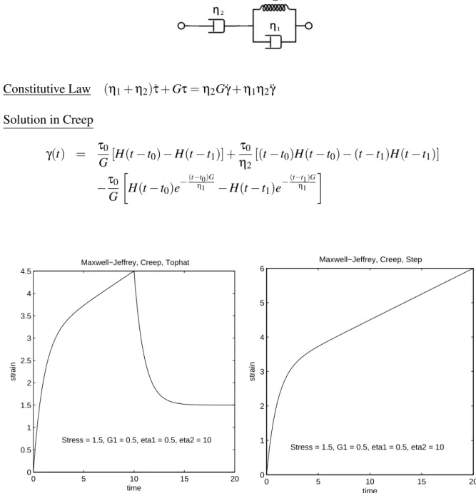
The measured strain in each model increases steadily under constant stress and relaxes to
a constant positive value after stress is removed, as seen in Figure 2.2 below. This
behav-ior comes from the free dashpot element present in series in each mechanical model. (Recall
that the dashpot is the viscous element.) Its presence leads to a factor of (t−t0) in the final
step stress solution, which causes the end behavior to go to infinity as t increases. A factor
of (t−t0)−(t−t1) appears in the final top hat stress solution. In this case, the two large
terms cancel ast goes to infinity, and the remaining terms are constant. Distinguishing the two
terms (besides the fact that the Two Parameter Maxwell model is completely linear, while the
Maxwell-Jeffrey model has curvature) is the sudden jump at the onset and offset of stress in
the Two Parameter Maxwell model.
The Two Parameter Maxwell Model
Mechanical Model
Constitutive Law λτ˙+τ=ηγ˙, whereλ=η/G Solution in Creep
γ(t) =λτ0
η [H(t−t0)−H(t−t1)] + τ0
η [(t−t0)H(t−t0)−(t−t1)H(t−t1)]
0 5 10 15 20
0.8 1 1.2 1.4 1.6 1.8 2 2.2 2.4 2.6
2 Param Maxwell, Creep, Tophat
Stress = 1.5, G1 = 1, eta1 = 20
time
strain
0 5 10 15 20
1.5 2 2.5 3
2 Param Maxwell, Creep, Step
Stress = 1.5, G1 = 1, eta1 = 20
time
strain
Figure 2.2: The Two Parameter Maxwell Model under a top hat (left) and step (right) stress.
The Maxwell-Jeffrey Model
Mechanical Model
Constitutive Law (η1+η2)τ˙+Gτ=η2Gγ˙+η1η2γ¨
Solution in Creep
γ(t) = τ0
G[H(t−t0)−H(t−t1)] +
τ0
η2[(t−t0)H(t−t0)−(t−t1)H(t−t1)]
−τ0
G ·
H(t−t0)e−
(t−t0)G
η1 −H(t−t
1)e−
(t−t1)G η1
¸
0 5 10 15 20
0 0.5 1 1.5 2 2.5 3 3.5 4 4.5
Maxwell−Jeffrey, Creep, Tophat
Stress = 1.5, G1 = 0.5, eta1 = 0.5, eta2 = 10
time
strain
0 5 10 15 20 0 1 2 3 4 5 6
Maxwell−Jeffrey, Creep, Step
Stress = 1.5, G1 = 0.5, eta1 = 0.5, eta2 = 10 time
strain
2.4 Linear Viscoelastic Solid Models
Solid-like materials are distinguished by their ability to store stress. This is reflected in a
response curve that recovers to zero strain when stress is removed - the stored stress pulls the
material back to its original shape. This behavior comes from the free spring element present in
parallel in each mechanical model. (Recall that the spring is the storage element.) However, it
is the absence of the free dashpot - which leads to the absence of factors of t - which contributes
to the long time recovery to zero behavior. Only step function and negative exponential terms
appear in the solutions. For larget, the negative exponential terms all approach 0. In step stress,
a single step function is left, causing the end behavior to asymptotically approach a positive
constant value. In top hat stress, the difference of two step functions remain (each having the
same magnitude), and so after long enough time, their difference approaches 0.
The 3 Parameter Maxwell or 3 Parameter Voigt models are good candidates for modeling
solid-like materials and are known as the linear viscoelastic solid models. Each fully recovers
to zero strain under a finite duration top hat stress, and each levels out to a steady state strain
under a constant applied stress. Each also has an initial jump in strain at the onset of an applied
stress and another jump at the offset of stress - another solid-like quality. The 2 Parameter Voigt
model is also categorized here for having similar end behavior. However, this model behaves
more like a fluid in that the initial strain begins at 0 and gradually rises (there is no sudden
jump). This may be good for modeling viscoelastic materials that have borderline viscous and
elastic properties.
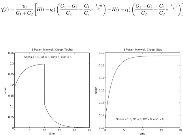
The Three Parameter Maxwell Model
Mechanical Model
Constitutive Law τ˙+λ1
1τ= (G1+G2)γ˙+
G2
λ1γ, whereλ1=η/G1
Solution in Creep
γ(t) = τ0
G1+G2
·
H(t−t0)
µ
G1+G2
G2 −
G1
G2e
−t−t0
λ1
−H(t−t1)
µ
G1+G2
G2 −
G1
G2e
−t−t1
λ1
¶¸
0 5 10 15 20 25
0 0.05 0.1 0.15 0.2 0.25 0.3 0.35
3 Param Maxwell, Creep, Tophat
Stress = 1.5, G1 = 3, G2 = 5, eta1 = 5
time
strain
0 5 10 15 20
0.13 0.14 0.15 0.16 0.17 0.18 0.19
3 Param Maxwell, Creep, Step
Stress = 1.5, G1 = 3, G2 = 8, eta1 = 6
time
strain
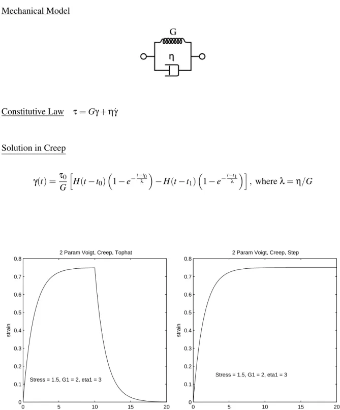
The Two Parameter Kelvin-Voigt Model
Mechanical Model
Constitutive Law τ=Gγ+ηγ˙
Solution in Creep
γ(t) =τ0
G h
H(t−t0)
³
1−e−t−λt0
´
−H(t−t1)
³
1−e−t−λt1
´i
, whereλ=η/G
0 5 10 15 20
0 0.1 0.2 0.3 0.4 0.5 0.6 0.7 0.8
2 Param Voigt, Creep, Tophat
Stress = 1.5, G1 = 2, eta1 = 3
time
strain
0 5 10 15 20
0 0.1 0.2 0.3 0.4 0.5 0.6 0.7 0.8
2 Param Voigt, Creep, Step
Stress = 1.5, G1 = 2, eta1 = 3
time
strain
Figure 2.5: The Two Parameter Kelvin-Voigt Model under a top hat (left) and step (right) stress.
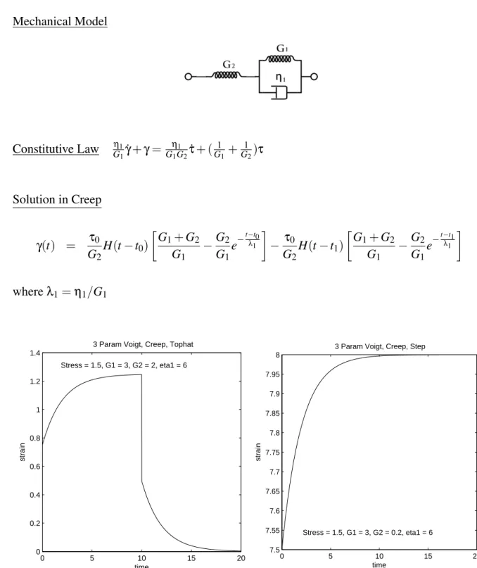
The Three Parameter Kelvin-Voigt Model
Mechanical Model
Constitutive Law η1
G1γ˙+γ= η1
G1G2τ˙+ (
1
G1+
1
G2)τ
Solution in Creep
γ(t) = τ0
G2H(t−t0)
·
G1+G2
G1 −
G2
G1e
−t−t0
λ1
¸
− τ0
G2H(t−t1)
·
G1+G2
G1 −
G2
G1e
−t−t1
λ1
¸
whereλ1=η1/G1
0 5 10 15 20
0 0.2 0.4 0.6 0.8 1 1.2 1.4
3 Param Voigt, Creep, Tophat
Stress = 1.5, G1 = 3, G2 = 2, eta1 = 6
time
strain
0 5 10 15 20
7.5 7.55 7.6 7.65 7.7 7.75 7.8 7.85 7.9 7.95 8
3 Param Voigt, Creep, Step
Stress = 1.5, G1 = 3, G2 = 0.2, eta1 = 6
time
strain
2.5 Summary of Model Signatures of Non-Inertial Creep
Ex-periments
Follow this guide for creep experiments done under a step or top hat stress to help choose the
best model to fit to your data. Refer to the figures above for examples of each model, and refer
to Section 4.2 for demonstrations of how each is used to fit experimental data.
1. Look at the terminal behavior of the strain response curve for your material. In top hat
stress, does it approach a positive finite steady state rather than recovering to zero? In
step stress, does it maintain positive slope rather than leveling off?
(a) If yes to either, the material exhibits fluid-like tendencies. Although the Two
Pa-rameter Maxwell model falls in this category, we do not recommend it. Refer
instead to the Maxwell-Jeffrey model and see #2.
(b) If the curve recovers to zero in top hat stress, or if it levels off in step stress, this
is a solid-like quality. The Two Parameter Voigt, Three Parameter Voigt, or Three
Parameter Maxwell model will capture this feature. See #3.
2. In either step or top hat stress, is there a sudden jump at time 0?
(a) If so, the Maxwell-Jeffrey model will not capture this jump, which is a solid-like
feature. If it is a significant factor in the data, you may need to refer to a solid-like
model (see #3) or a model not discussed in this thesis (perhaps a 4 parameter or
nonlinear model).
(b) If the initial value is 0, try theMaxwell-Jeffreymodel first, which also exhibits a
gradual decline upon the removal of stress.
3. Does the strain response curve have a sudden jump at time 0 in either top hat or step
stress?
(a) If so, the Three Parameter Maxwell and Three Parameter Voigt models can
both capture this feature, which is also a solid-like feature. These two models are
essentially the same, and in addition they exhibit a sudden drop upon the removal
of stress.
(b) If instead the curve begins close to zero, try theTwo Parameter Voigtmodel. This
model is fluid-like in the way the strain gradually rises from 0, and solid-like in the
Chapter 3
Inertial Models
3.1 Overview of Inertial Models
In creep experiments that utilize instrumental inertia, a Rheometer imparts a controlled stress
on the material, and the undamped inertia of the instrument is allowed to enhance the elasticity
of the material, causing ringing behavior to occur. The rheometer measures angular
displace-ment as the material is allowed to relax and converts this to a measuredisplace-ment of compliance, as
seen previously in non-inertial creep. Strain is plotted against time to produce a response curve
with similar overall features as in non-inertial creep, with the addition of oscillatory behavior.
The oscillations mimic a specific frequency, and storage and loss properties are extracted for
how the material would behave at this frequency under a sinusoidal driving force. This
fre-quency is much higher than in the very low frefre-quency non-inertial creep experiments. As a
result, useful information can be extracted more quickly, meaning the experiments take less
time. This is an appeal of inertial creep.
In inertial creep, a parameterαnot seen in the non-inertial models is present. This param-eter represents the inertia of the instrument. Theoretically it is a known paramparam-eter, however it
is difficult to determine its value for the instrument and is therefore usually included in the list
of parameters to be fit in the model. Different ringing characteristics in the responses can
of the instrument: Inertial Maxwell, Inertial Voigt and Inertial Maxwell-Jeffrey. Each model
corresponds to a linear differential constitutive law which can be solved in closed form.
The models, the corresponding constitutive laws, and their solutions under a step stress are
given in Section 3.3 below. The stress function is given byτ(t) =τ0H(t−t0). Solutions under
a step stress rather than a top hat stress, as in Sections 2.3 and 2.4, are given here for simplicity
due to the fact that inertial solutions are much longer then non-inertial solutions and top hat
solutions would require twice as many terms. Additionally, one may notice that the inertial
constitutive laws presented here do not contain γ- this is a result of the way in which inertial problems must be handled, which is discussed in the example derivation in Section 3.2 below.
3.2 Example: Coupling of Instrumental Inertia to Maxwell
Model and Derivation of Analytical Solution
We refer to (Barav98) for a more thorough explanation on coupling viscoelasticity and
instru-mental inertia. Here, we give the mathematical details of how to derive the coupled constitutive
law for the Two Parameter Maxwell model, followed by the steps for solving the model for the
strain, given an applied step stress.
We need an equation to describe the motion of the rotating part of the rheometer. Newton’s
second law, given in rotational terms, is
Idθ˙
dt =ΓA−ΓR (3.1)
whereI is the moment of inertia of the rotating rod and cone in the machine, ˙θis the angular velocity,ΓAis the applied torque, andΓRis the resistive torque due to the sample. This general
law can be written in terms of stress and strain as
whereα=IFτ
Fγ˙ is a constant, Fτ is the proportionality factor between shear stress and torque,
andFγ˙ is the proportionality factor between shear rate and angular velocity. Equation (3.2) is
what we wish to couple to the constitutive law for the Two Parameter Maxwell model, reprinted
here,
λτR˙ +τR=ηγR˙ (3.3)
Equation (3.2) is an equation for ¨γ. The logic for solving this inertial problem is to substitute (3.2) into (3.3) after differentiating (3.3) once. This gives us
λτ¨R+τ˙R=η
µ 1
ατA−
1
ατR
(3.4)
The goal is to eliminateγfrom the equation and obtain an expression forτR. Once we findτR, we can substitute it back into Equation (3.2) to solve for γ. If we let the applied stress be a shear step stress,τA=τ0H(t), then we have
λτR¨ +˙τR+η ατR=
η
ατ0H(t) (3.5)
The solution to the second order differential equation of (3.5) will have oscillating and
non-oscillating regimes (that is, it will have one solution containing sines and cosines, and one
con-taining hyperbolic sines and hyperbolic cosines). Oscillations will exist for 12−4(λ)(η/α)≤
0, or, rearranging, forG≤ 4ηα2 (recallλ=η/G). Now, when we coupled the equations we lost
γ(t), and we have remaining an equation that we wish to solve forτ(t).
To begin, we take the Laplace Transform of (3.5) and solve forT(s), obtaining,
T(s) =τ0
³η
α
´ 1
s(λs2+s+η
α)
(3.6)
We use partial fractions to break up the denominator. Observe,
1 s(λs2+s+η
α)
= A
s +
Bs+C
λs2+s+η
α
1 = A
³
λs2+s+η α
´
+ (Bs+C)s
We solve forAfirst by lettings=0:
1 = A
³
λ02+0+η α
´
+ (B∗0+C)∗0
1 = Aη
α
A = α
η
Next, we solve forBandCby equating coefficients of thes2andsterms respectively, and using A= αη. Fors2we have
0 = Aλ+B
0 = α
η η
G+B
B = −α
Equating coefficients forswe have
0 = A+C
0 = α
η+C
C = −α
η
Now we can rewrite equation (3.6) as partial fractions:
T(s) =τ0
³η
α
´Ãα/η
s +
−α
G s+−ηα
λs2+s+η
α !
(3.7)
which simplifies as
T(s) =τ0
µ 1 s −
s+G/η
s2+ (G/η)s+G/α
(3.8)
To find the inverse Laplace Transform, we must manipulate equation (3.8) into a form for
which we recognize inverses. First we split up the large fraction:
T(s) =τ0
µ 1 s−
s
s2+ (G/η)s+ (G/α)−
G/η
s2+ (G/η)s+ (G/α)
(3.9)
Next we perform completing the square on the denominators:
T(s) = τ0
µ 1 s−
s
s2+ (G/η)s+ (G/2η)2+ (G/α)−(G/2η)2
− G/η
s2+ (G/η)s+ (G/2η)2+ (G/α)−(G/2η)2
= τ0
1
s−
s
(s+G/2η)2+G
α− G
2
4η2
− G/η (s+G/2η)2+G
α− G
2
4η2
Lastly, we require that the s in the numerator of the middle term be shifted by G/2η to
match the s in the denominator. Thus, we add and subtract G/2η to the middle term and simplify:
T(s) = τ0
1
s−
s+G/2η−G/2η (s+G/2η)2+G
α− G
2
4η2
− G/η (s+G/2η)2+G
α− G
2
4η2
= τ0
1
s−
s+G/2η (s+G/2η)2+G
α− G
2
4η2
− G/2η (s+G/2η)2+G
α− G
2
4η2
(3.10)
Now we are ready to take the inverse Laplace Transform. The first term will transform back
to 1, the second term is a cos(t)term, and the last term is a sin(t)term. Additionally, the cos and sin terms are shifted byG/2η, which results in an exponential terme−2Gηt to appear in the
inverse transform. The final result is
τ(t) =τ0
µ
1−e−2Gηt
·
cos(ωt) + G
2ηωsin(ωt)
¸
(3.11)
whereω=
q
G
α− G
2
4η2.
Knowing τwe can now back solve forγ. We substitute equation (3.11) for τR andτ0H(t)
forτA into equation (3.2) to find an expression forγ,
¨
γR= σα0
·
H(t)−1+e−2Gηt
µ
cos(ωt)− G
2ηωsin(ωt)
¶¸
(3.12)
Integrating from 0 tottwice, we obtain the final solution:
γ(t) = τ0 η
· t− a
G µ G η − η a ¶ ·
1−e−2Gηt
µ
cos(ωt) + G
2ηω
G/η−3η/a
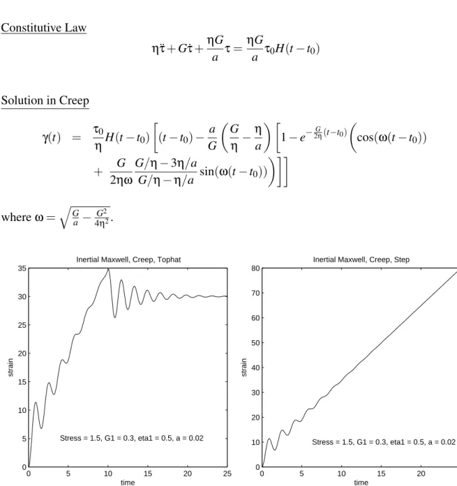
3.3 List of Inertial Models
The Inertial Maxwell Model
Constitutive Law
ητ¨+Gτ˙+ηG
a τ=
ηG
a τ0H(t−t0)
Solution in Creep
γ(t) = τ0
ηH(t−t0)
·
(t−t0)− a
G µ G η− η a ¶ ·
1−e−2Gη(t−t0) µ
cos(ω(t−t0))
+ G
2ηω
G/η−3η/a
G/η−η/a sin(ω(t−t0)) ¶¸¸
whereω=
q
G a− G
2
4η2.
0 5 10 15 20 25
0 5 10 15 20 25 30 35
Inertial Maxwell, Creep, Tophat
Stress = 1.5, G1 = 0.3, eta1 = 0.5, a = 0.02
time
strain
0 5 10 15 20 25
0 10 20 30 40 50 60 70 80
Inertial Maxwell, Creep, Step
Stress = 1.5, G1 = 0.3, eta1 = 0.5, a = 0.02
time
strain
Figure 3.1: The Inertial Maxwell Model under a top hat (left) and step (right) stress.
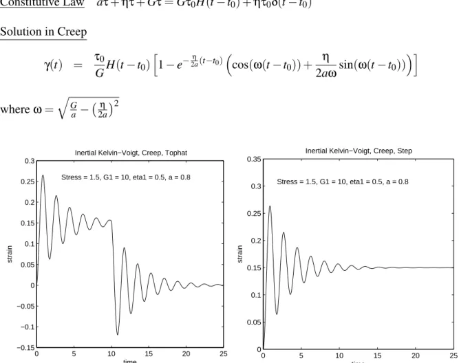
The Inertial Kelvin-Voigt Model
Constitutive Law aτ¨+η˙τ+Gτ=Gτ0H(t−t0) +ητ0δ(t−t0)
Solution in Creep
γ(t) = τ0
GH(t−t0) h
1−e−2ηa(t−t0) ³
cos(ω(t−t0)) + η
2aωsin(ω(t−t0))
´i
whereω=
q G a− ¡η 2a ¢2
0 5 10 15 20 25
−0.15 −0.1 −0.05 0 0.05 0.1 0.15 0.2 0.25 0.3
Inertial Kelvin−Voigt, Creep, Tophat
Stress = 1.5, G1 = 10, eta1 = 0.5, a = 0.8
time
strain
0 5 10 15 20 25
0 0.05 0.1 0.15 0.2 0.25 0.3 0.35
Inertial Kelvin−Voigt, Creep, Step
Stress = 1.5, G1 = 10, eta1 = 0.5, a = 0.8
time
strain
The Inertial Maxwell-Jeffrey Model
Constitutive Law
(η1+η2)τ¨+ (G+η1η2
a )˙τ+ Gη2
a τ =
Gη2
a τ0H(t−t0) +
η1η2
a τ0δ(t−t0) Solution in Creep
γ(t) = τ0H(t−t0)
· t−t0
η2 −B+e
−A(t−t0) µ
Bcos(ω(t−t0)) +ωA(B−A1η
2)sin(ω(t−t0))
¶¸
whereω=
q η2G
a(η1+η2)−A
2,A= aG+η1η2
2a(η1+η2), andB=
a(η1+η2) η2G
³
2A
η2 −
1
a
´ .
0 5 10 15 20 25
0 0.5 1 1.5 2 2.5 3
Inertial Maxwell−Jeffrey, Creep, Step
Stress = 1.5, G1 = 5, eta1 = 0.05, eta2 = 15, a = 0.3
time
strain
Figure 3.3: The Inertial Maxwell-Jeffrey Model under a top hat (left) and step (right) stress.
3.4 Summary of Model Signatures of Inertial Creep
Experi-ments
Follow this guide to help choose the best inertial model to fit to your data taken under either
a top hat stress or a step stress. Refer to the figures above for examples of each model, and
see Section 4.2 for demonstrations of how each is used to fit experimental data. Note that
the items to distinguish between the inertial models are essentially the same (after
consider-ing the oscillations) as the non-inertial models. Note also that the Inertial Maxwell and Inertial
Maxwell-Jeffrey models are identical in graphical behavior, whereas in the non-inertial regimes
the models from which these are derived are quite different. Because of this similarity, there
are essentially only two inertial graphs given here to choose from, and thus only one feature
is required to distinguish the two. Two separate features are given here, the first dealing with
end behavior and the second dealing with the transition when stress is turned off. These two
features rely heavily on the distinction between liquid-like and solid-like behavior, as there are
no intermediate options having a mix of characteristics (as in the Two Parameter Voigt model
for the non-inertial options).
1. Look at the terminal behavior of the response curve for your material. In step stress, does
it level off at some finite steady state value? In top hat stress, does it recover to zero?
(a) If yes, try theInertial Kelvin-Voigtmodel. The material exhibits solid-like
behav-ior.
(b) If the oscillations have an overall positive slope in step stress, or recover to a
pos-itive steady state in top hat stress, try either theInertial Maxwell or the Inertial
Maxwell-Jeffreymodel. These are liquid-like behaviors.
removed?
(a) If the oscillations jump from one baseline value down to zero at the time when the
stress is turned off (a solid-like behavior), try theInertial Kelvin-Voigtmodel.
(b) If the oscillations switch from steadily increasing to leveling off around some
non-zero value (no sudden jump is a liquid-like behavior), try either theInertial
Maxwellor theInertial Maxwell-Jeffreymodel.
Chapter 4
Software Tools
4.1 Parameter Inference and Analysis of Parameters Using
Mathematica
Each model discussed in this thesis has either two or three fundamental parameters that
com-pletely determine the final shape of the curve. The parameters are chosen from G1, G2, η1,
orη2. For a given model, it is expected that each parameter may have a strong effect on the
shape of the curve (that is, changing the value of this parameter by small amounts causes larger
changes to the shape) or may have only a weak affect on the shape of the curve (the curve will
look similar across a wide range of values for this parameter). Knowing which parameters have
strong and weak affects may help in analyzing the parameter fittings of experimental data. For
example, it may influence the decision of when to hold a known value constant versus when to
let it iterate.
To get an idea of how each parameter affects the shape of a given model, Mathematica
can be used to create dynamic plots of each model. The function ‘Manipulate’ is used in
conjunction with ‘Plot’ to create a graph of the model along with slider bars for each parameter
in the model. The graph changes as the sliders are altered. The code for this is only two lines.
slider.
F u n c t i o n N a m e [ param1 , . . . ] : = e q u a t i o n
M a n i p u l a t e [ P l o t [ F u n c t i o n N a m e [ p a r a m e t e r s ] ,{t , 0 , 2 0}, P l o t R a n g e
−>{0 ,5}] ,{Param1 , min , max} , . . . ]
For example, to generate a dynamic plot of the compliance for the Two Parameter Voigt
model, the following can be used:
CRVoigt2 [ G , n ] : = ( 1 / G)∗( U n i t S t e p [ t ]∗( 1 − Exp [−( t∗G) / n ] ) −
U n i t S t e p [ t − t e n d ]∗( 1 − Exp [−(( t − t e n d )∗G) / n ] ) )
M a n i p u l a t e [ P l o t [ CRVoigt2 [G, e t a ] , {t , 0 , 2 0}, P l o t R a n g e −> {0 ,
1 . 5}] , {G, 0 , 5}, {e t a , 0 , 5}]
After adjusting the parameter values, the output will look similar to Figure 4.1 below.
Parameter sensitivity is affected by values of other parameters
Through observation, it is found that the effects of a parameter on the graph depend on several
factors. First, characterizing the effects of a parameter depends on whether the parameter is in
a high or low regime as well as whether the remaining parameters are at high or low values.
Consider the Three Parameter Voigt model,
γ(t) = 1
G2H(t−t0)
·
G1+G2
G1 −
G2
G1e
−(t−t0)G1
η
¸
− 1
G2H(t−t1)
·
G1+G2
G1 −
G2
G1e
−(t−t1)G1
η
¸
We observe thatη, which is seen in the denominator of the exponential, affects the sharpness of the curve - smaller values of ηcause a larger exponent and generate a steeper curve. The parameterG1is also related to the exponent, as well as the magnitude of the entire curve. Thus,
whenηis very small (leading toward a sharp curvature), small values ofG1 counteractηand
lead to a more gradual curvature. In this realm, small changes in G1 can cause the curve to
look very different. Forη=2 andG2=2, compare the curves in Figure 4.2 whenG1changes
from 0.5 to 1.5, a step of one unit.
On the other hand, whenG1is larger thanη, it amplifies the effect thatηalready has on the
graph and produces a very steep initial rise followed by a sudden flattening out. In this realm
(smallη, largeG1), the ratio Gη1 is already so large that even large changes inG1 have a very
small effect on the overall shape of the curve. Forη=2 and G2=2, compare the curves in
Figure 4.3 whenG1changes from 20 to 30, a step of 10 units.
This interaction between parameters can be explained by realizing that, in each model, the
pieces that really affect the shape of the graph are functions of the basic parametersG1,G2,η1
orη2. As a simple example, consider the equation of a line, y=mx+b. Here, mdefines the
slope andbdefines the y-intercept. However, if you are concerned with two different
parame-ters, sayhandg, wherey= hgx+h, then the slope is no longer defined by a single parameter. The linear viscoelastic models considered here are for the most part more complicated than a
Figure 4.2: The Three Parameter Voigt model changes noticeably for small changes inG1when
G1is small compared toη.
Figure 4.3: The Three Parameter Voigt model changes very little for changes inG1whenG1is
simple line, and thus the interactions between parameters are even more intricate.
Parameter analysis is affected by which graphical features are important
Parameter sensitivity also depends on what features of the graph are important for analyzing
the data. For instance, in fluid models often the slope of the compliance curve after a long
time step stress or the value to which the fluid recovers after stress is removed are important
indicators of the viscosity of the fluid. If this is all that needs to be observed from the data,
then any parameters not directly affecting the long time slope may be unimportant. It could
be said that these parameters are not sensitive to the prediction of the viscosity. However, any
parameters affecting the end behavior will need to be considered more closely.
The Maxwell-Jeffrey model is a linear viscoelastic fluid model which exhibits a constant
slope in long times while constant stress is applied, and recovers to a positive steady state
after the removal of stress. It can easily be observed using Mathematica that out of the three
parameters creating the Maxwell-Jeffrey model, G,η1 andη2, onlyη2 changes the long time
end behavior. This is verified by looking at the equation,
γ(t) = 1
G[H(t−t0)−H(t−t1)] + 1
η2[(t−t0)H(t−t0)−(t−t1)H(t−t1)]
−1
G ·
H(t−t0)e−
(t−t0)G
η1 −H(t−t
1)e−
(t−t1)G η1
¸
and noticing thatη2is the only parameter affecting the second term, which is the only term that
does not go to zero ast increases. The largerη2 is, the smaller the slope and/or steady state
value of the end behavior. Thus, if you are trying to model this end behavior, you will need to
estimateη2to high accuracy while the other parameters could be allowed to vary greatly.
Figure 4.4: Forη2=14 (left figure), the slope of the end behavior (as well as the steady state
value) are much higher than for η2=40 (right figure). G affects the overall magnitude of
the stress-on part of the graph, andη1 affects the curvature, but neither Gnor η1 affects end
behavior.
Parameter inference is influenced by the fitting region
During the fitting process, parameter sensitivity is also influenced by the size of the region you
are fitting to, and which particular features are captured in this region. The region must be large
enough to capture some defining features of the data, but must be small enough to prevent the
fitting algorithm from crashing. That is, you cannot always simply fit over the entire domain
of the data. It is important to consider these two things (length and position of fitting interval)
because parameters do not affect all regions of a graph in the same way.
Reconsider the Maxwell-Jeffrey model. In the table below, large error bars were introduced
to the Maxwell-Jeffrey model having the true parametersG=1,η1=2, andη2=12 to try to
determine how much random error could be present while still predicting accurate parameter
values. Data was generated for 10%, 30% and 50% random error, and the parameter fitting gui
from (Xu2009) was used to recover the parameters in the intervalt= (0,5).
Figure 4.5: Even at 50% random error,Gandη1 remain close to their true values of 1 and 2,
respectively. However,η2deviates, likely due to the early fitting window.
in the previous section. We have demonstrated that η2 is responsible for changing the end
behavior. However, the fitting interval(0,5)does not include information on the end behavior. That is, a good fit can be made in(0,5)for a range of values of η2because changes inη2do
not affect this part of the graph. Figure 4.6 demonstrates how values ofη2from 8 to 15 do not
change the fitting region very greatly.
Related to this issue is the usage of fitting intervals which are too small. The same
Maxwell-Jeffrey model with parametersG=1,η1=2, andη2=12 was fit in the small intervalt= (7,8).
This returned parameter estimates of G∗=0.012, η∗1=−0.678, and η∗2=0.558. Figure 4.7 shows how the the two models align very closely on the interval (7,8); however, the model generated byG∗,η∗
1andη∗2is vastly different from the original data, as Figure 4.8 shows.
4.2 Generating Experimental Error: Make Data Tool
The data obtained from creep experiments is expected to be nonlinear, which can be supported
by the observation of parameter walk-offs, as demonstrated in (Xu2009). Thus, these linear
models cannot be expected to match the data exactly. In addition, experimental data is noisy,
and this may interfere with the fitting algorithm. To examine whether simple random error
could be added to an exact model to reflect the noise in raw data, we added functionality to
the parameter fitting gui from (Xu2009) which allows a user to choose a model, enter a value
0 2 4 6 8 10 −0.5
0 0.5 1 1.5 2 2.5
time
compliance
A Jeffrey model with 3 different values of eta2 G = 1, eta1 = 2, eta2 = 12
G = 1, eta1 = 2, eta2 = 8 G = 1, eta1 = 2, eta2 = 15
Figure 4.6: Observe that the three graphs, created by varyingη2between 8 and 15 and holding
the other parameters constant, are slow to spread out. This means that the closer the fitting interval is to 0, the better any value ofη2between 8 and 15 could generate a reasonable fit.
4 5 6 7 8 9 10 11 0.8
1 1.2 1.4 1.6 1.8 2
time
compliance
Coinciding region for two different Maxwell−Jeffrey graphs
True Data (G=1, eta1=2, eta2=12)
Model with parameters from fitting to [7:8] window