Mode System Effects in an Online Panel Study: Comparing a Probability-based Online Panel with two Face-to-Face Reference Surveys

Mode System Effects in an Online Panel

Study: Comparing a Probability-based

Online Panel with two Face-to-Face

Reference Surveys

Bella Struminskaya

_{, Edith de Leeuw}

_&

Lars Kaczmirek

1

GESIS – Leibniz Institute for the Social Sciences

2

Department of Methodology and Statistics, Utrecht University

Abstract

One of the methods for evaluating online panels in terms of data quality is comparing the estimates that the panels provide with benchmark sources. For probability-based online panels, high-quality surveys or government statistics can be used as references. If differ-ences among the benchmark and the online panel estimates are found, these can have sev-eral causes. First, the question wordings can differ between the sources, which can lead to differences in measurement. Second, the reference and the online panel may not be com-parable in terms of sample composition. Finally, since the reference estimates are usually collected face-to-face or by telephone, mode effects might be expected. In this article, we investigate mode system effects, an alternative to mode effects that does not focus solely on measurement differences between the modes, but also incorporates survey design fea-tures into the comparison. The data from a probability-based offline-recruited online panel is compared to the data from two face-to-face surveys with almost identical recruitment protocols. In the analysis, the distinction is made between factual and attitudinal questions. We report both effect sizes of the differences and significances. The results show that the online panel differs from face-to-face surveys in both attitudinal and factual measures. However, the reference surveys only differ in attitudinal measures and show no significant differences for factual questions. We attribute this to the instability of attitudes and thus show the importance of triangulation and using two surveys of the same mode for com-parison.

Keywords: mode system effect, online panel, benchmark survey comparison, data quality

Direct correspondence to

Bella Struminskaya, GESIS – Leibniz Institute for the Social Sciences, B 2,1, 68159 Mannheim, Germany

E-mail: [email protected]

1 Introduction

Several large-scale panel and repeated cross-sectional surveys incorporate or are planning to incorporate an online mode for data collection to reduce costs or to maximize contact and response rates. Some panels are designed as online panels from the beginning, with an interviewer-administered panel recruitment procedure and web-based data collection for the surveys in the panel (e.g., the LISS Panel1 in the Netherlands and the KnowledgePanel2 _{of GfK Custom Research, formerly} Knowledge Networks in the United States). Other panels switch from interviewer-administered to online mode for their data collection (e.g., the Netherlands Kin-ship Panel Study3_{), employ an additional online component (e.g., ANES 2008-2009} Panel Study4_{), or experiment with including an online mode along with interview} modes (ESS experiments on mixing modes5_{, Understanding Society Innovation} Panel in the UK6_{, and Labor Force Survey and Crime Victimization Survey in the} Netherlands7_).

Data users need to know that irrespective of the mode in which data were col-lected, it is possible to make valid inferences about the processes that data users study, and that panel or trend data are comparable, that is, not influenced by the mode change.

In the literature on survey data collection modes, key dimensions are discerned on which modes vary that account for differences in responses across modes. In her theoretical model on mode effects, de Leeuw (1992, 2005) identified three sets of factors that explain differences between the modes: (1) media-related factors, (2) factors that are related to information transmission, and (3) interviewer effects. Media-related factors encompass social conventions and customs associated with the media utilized in survey methods. Media-related factors include socio-cultural

1 http://www.lissdata.nl/lissdata/

2 http://www.knowledgenetworks.com/knpanel/

3 http://www.nkps.nl/NKPSEN/nkps.htm; see also Hox, de Leeuw, & Zijlmans (2015). 4 http://www.electionstudies.org/studypages/2008_2009panel/anes2008_2009panel.

htm

5 http://www.europeansocialsurvey.org/methodology/mixed_mode_data_collection. html

6 https://www.understandingsociety.ac.uk/about/innovation-panel; see also Auspurg et al. (2013)

effects such as familiarity with a medium, patterns of use of the medium, as well as norms of social interaction (e.g., interviewers having more control over the inter-viewing process and pace because they initiate the interaction). Factors related to information transmission involve more technical aspects of the communication process and include the manner in which information is presented (visual presenta-tion, auditory presentation or both visual and auditory) as well as additional cues that are pertinent to the question-answering process (such as text and lay-out in the self-administered mode, gestures and tone of the interviewer in the face-to-face mode). The third set of factors includes the influence of an interviewer on the responses provided by respondents. Interviewer-administration can influence the respondents’ feelings of privacy and lessen their willingness to disclose sensitive information. On the other hand, interviewers can provide clarification or motivate respondents to provide answers. In a meta-analysis of 52 early mode comparison studies, de Leeuw (1992, chapter 3) found that face-to-face and telephone inter-views did not differ in response validity through record checks and on social desir-ability. When both interview modes were compared with self-administered mail surveys, the meta-analysis revealed an interesting picture. It is somewhat harder to have people answer questions in a self-administered mode (both response rate and item missing rates are higher), but the resulting answers show less social desirabil-ity and more openness on sensitive topics. These results emphasize the importance of the role of the interviewer.

Groves, Fowler, Couper, Lepkowski, Singer, and Tourangeau (2009) identify five dimensions along which data collection methods differ that partly overlap with the dimensions discussed above: (1) the degree of interviewer involvement, (2) the level of interaction with the respondent, (3) the degree of privacy for the respon-dent, (4) the channels of communication used, and (5) the degree of technology use. Compared to the interviewer-administered methods of data collection, online sur-veys eliminate interviewer involvement and offer a high level of privacy, and impose a low cognitive burden, because the questions can be easily reread on the computer screen (Tourangeau, Conrad, & Couper, 2013). In their meta-analysis of studies employing randomized experiments to compare different modes, Tourangeau et al. (2013) conclude that compared to interviewer-administered surveys, online surveys yield more reports of sensitive information and that compared to paper-and-pencil surveys, only small advantages are offered by online surveys. This finding is con-sistent with the finding of Klausch, Hox, & Schouten (2013), who find measurement differences between interviewer- and self-administration that are absent when com-paring face-to-face to the telephone mode and mail to the online mode. It is also in line with the results of the early meta-analysis by de Leeuw (1992), and suggests a dichotomy in modes with and modes without an interviewer.

mode (see also the meta-analyses by de Leeuw, 1992 and Tourangeau et al, 2013). These studies focus on a particular source or error (e.g., measurement error), inves-tigate a particular mechanism that produces a mode difference (e.g., social desir-ability), and aim at estimating pure mode effects (Biemer & Lyberg, 2003, p. 207; Couper, 2011, p. 894-897).

However, in daily practice, associated with each mode is a set of decisions intended to take advantage of the benefits of each mode (Lyberg & Kasprzyk, 1991, p. 249) and in addition to mode other factors will vary, such as number of calls ver-sus number of reminders in interview vs. web modes. Consequently, a good alter-native is to measure a mode system effect, that is, to compare whole systems of data collection developed for different modes. A data collection system is defined as an “entire data collection process designed around a specific mode” (Biemer & Lyberg, 2003, p. 208; Biemer, 1988). A small number of studies focuses on the outcomes, examining total survey systems, where the final survey estimates are compared (Couper, 2011), and these studies are especially important for practitio-ners who want to switch from one mode of data collection to another (e.g, from interview to online survey) or employ a mixed-mode system for data collection.

In this study, we investigate mode system effects of three data collection systems, comparing the data from an online panel to two face-to-face reference surveys. Central is the question whether the different systems produce equivalent results given all the differences in data collection. Data from surveys that are car-ried out in different modes may differ for three reasons (de Leeuw & Hox, 2011, p. 53). Firstly, differences may be caused by the implementation of different question formats in different modes (question effects), secondly, different modes may lead to a different sample composition (selection effects), and, thirdly, the modes them-selves may lead to the different response processes (mode effect).

In order to systematically investigate mode sysytem effects, we focus our com-parison on questions with the same question wording and control step-by-step for differences in sample composition. As reference we use data from two face-to-face interview surveys, whose recruitment and administrative procedures are similar. Based on the mode comparison studies and meta-analyses cited above, we do not expect differences in the estimates based on the face-to-face interviews after adjust-ing for potential sample composition differences. However, we do expect differ-ences in estimates based on data collected online compared to the estimates based on the reference interview surveys (Hypothesis 1).

about an issue – considerations that have different levels of accessibility. While forming an answer, respondents process these considerations, which requires delib-eration and effort (Tourangeau, Rips, & Rasinski, 2000, pp. 179-180). In a face-to-face survey, an interviewer initiates the interaction and thereby controls the pace of the interview (de Leeuw, 2005), so the time might not be sufficient for a respondent to process the considerations needed to generate responses to an attitudinal ques-tion. In a self-administered online survey, by contrast, the respondent controls the survey situation, including the pacing, which allows for taking more time if needed to answer an attitudinal question. Furthermore, according to Tourangeau, Conrad, and Couper (2013), online surveys impose a lower cognitive burden on the respon-dent due to the visual presentation of information, allowing responrespon-dents to consider the question and response alternatives better. In an experimental study specifically designed to evaluate mode effects in which respondents were randomly assigned to mail, web, telephone and face-to-face conditions in the Crime Victimization Survey of the general population in the Netherlands, Klausch, Hox, and Schouten (2014) indeed find measurement differences for attitudinal variables such as ques-tions about the social quality and problems of the neighborhood, and no measure-ment differences for two factual variables on victimization.

We therefore expect that mode system effects between online and face-to-face interviews are more pronounced in attitudinal questions than in factual questions (Hypothesis 2).

2 Data

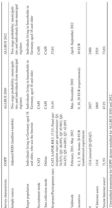
We use data from the GESIS Online Panel Pilot8_{, a probability-based online panel} of Internet users in Germany; we use two cross-sections from the German General Social Survey (ALLBUS 2010 and ALBUSS 2012) as reference surveys. Table 1 contains an overview of design characteristics for the GOPP and the reference sur-veys.

GESIS Online Panel Pilot (GOPP)

The GESIS Online Panel Pilot (GOPP) is a telephone-recruited online panel of Internet users aged 18 and older who live in private households in Germany. To recruit participants, the randomized last digit method was used, which is a varia-tion of a random digit dialing (RDD) for Germany (Gabler & Häder, 2002). A dual-frame approach was used: the samples were drawn independently from landline and mobile phone frames, aiming at a final sample with 50% eligible landline numbers and 50% eligible mobile phone numbers. In order to handle the overlap between the

two frames, the inclusion probabilities for target persons were calculated accord-ing to the formulas of Siegfried Gabler, Sabine Häder and their colleagues under the assumption of independence of the two samples (Gabler, Häder, Lehnhoff, & Mardian, 2012). The inclusion probabilities account for the sample sizes and frame sizes of both landline and mobile phone components, as well as for the number of landline and mobile phone numbers at which a respondent can be reached. For the landline component, household size was also included in the calculation. The target person, that is, the person with the most recent birthday, provided this information. For the mobile phone component, no selection procedures were implemented, since mobile phone sharing in Germany is approximately 2% (Gabler et al. 2012).

The recruitment took place in three sequential study parts using almost identi-cal recruitment protocols. Recruitment periods were in February 2011, in June-July 2011, and in July-August 2011. After a short telephone interview, respondents were asked to provide their email addresses in order to join an online panel. Respondents who agreed would then be sent email invitations to online surveys of 10-15 minutes every month for eight months in total. Prospective panel members were offered incentives of 0, 2, 5, or 10 Euros, which were varied experimentally. An additional bonus of 20 Euros for completing all eight online questionnaires was offered.

In the GESIS Online Panel Pilot questionnaires, a number of questions were replicated from other well-known social surveys. The first goal of such replication was to assess the feasibility of surveying rather complex constructs in an online set-ting. The second goal was to study data quality by comparing online estimates to external benchmarks. A substantial part of questions originated from the German General Social Survey (“ALLBUS”) 2010. The original question wordings were retained, except for the cases when an adjustment was needed to make questions suitable for a self-administered mode. It is furthermore important to note that every questionnaire in the GOPP had a leading topic and most questions were asked once. Questions for analysis were selected from questionnaires (waves) 1, 2, 3, 4, 5, and 7.

German General Social Survey “ALLBUS”

The German General Social Survey is a general population survey on attitudes, behavior, and social structure in Germany. It has been conducted by GESIS bian-nually since 1980. The survey mode is face-to-face interviewing. For our analy-ses, we use ALLBUS 20109 _{and ALLBUS 2012}10_{, which both implemented a} two-stage disproportionate random sample of individuals living in private households in Germany, aged 18 and older. The data collection for both ALLBUS 2010 and ALLBUS 2012 was conducted by the same fieldwork agency, using similar pro-cedures for contacting and interviewing the respondents. A difference is that in

ALLBUS 2010, an incentive experiment was employed in which respondents could receive 10 Euros, 20 Euros, or no incentive (Wasmer, Scholz, Blohm, Walter, & Jutz, 2012, p. 51), whereas in ALLBUS 2012, all respondents were paid 10 Euros. It should be noted the target population of ALLBUS consists of both Internet and non-Internet users. A question on private Internet use is asked in both ALLBUS surveys. For our analysis, we are therefore able to compare GOPP with full samples of the ALLBUS surveys and with the subsamples of Internet users.

ALLBUS contains item batteries and single questions on opinions, which are repeated over the years in order to analyze social trends. The wording of the demo-graphic questions generally does not change between ALLBUS surveys. Overall, the overlap in questions between ALLBUS 2010 and ALLBUS 2012 is 82 ques-tions, 46 of which are not preceded by one or multiple filter questions11_{, that is, 46} questions that were asked both in ALLBUS 2010 and in ALLBUS 2012 were posed to the total sample.

3 Measures

For the mode system comparison, we made a careful selection of factual and atti-tudinal questions from ALLBUS 2010 to avoid question format effects. About 73 questions from ALLBUS 2010 were also asked in the GESIS Online Panel Project. However, only a subset of these questions was asked in ALLBUS 2012. Only ques-tions that were present in both ALLBUS 2010 and 2012 and were replicated in the GOPP are analyzed. These questions were not repeatedly measured in GOPP but distributed over the questionnaires, so that each question that we use for compari-son was asked only once in the online panel. This prevents possible confounding of the answers due to learning effects (panel conditioning). We carefully inspected the questions and only included questions that had the same question wording (see Appendix for details) and were asked of the whole sample, that is, were not pre-ceded by filter questions.

In total, 12 attitudinal and 7 factual questions fit these criteria. Attitudinal questions included respondents’ assessment of the current economic situation in Germany and the economic situation in one year, the assessment of respondents’ own financial situation and prospective financial situation in one year, general health, religiosity, self-assessed social class, four general attitude questions on soci-etal functioning (anomie), and political orientation (right-left).

Ta bl e 1 Sa m pl e a nd s ur ve y d es ig n d esc rip tio n f or G O PP a nd A LL BU S s ur ve ys Su rv ey ch ar ac te ris tic G OPP A LL BU S 2 010 A LL BU S 2 01 2 Sa m pl e sou rc e A dj us te d R DD ( la nd lin e+ m ob ile ) Tw o-sta ge p ro ba bi lity : m un ic ip ali -tie s a nd i nd iv id ua ls f ro m m un ic ip al re gi ste rs Tw o-sta ge p ro ba bi lity : m un ic ip ali -tie s a nd i nd iv id ua ls f ro m m un ic ip al re gi ste rs Ta rg et p op ul at ion In di vi du al s l iv in g i n G er m an y a ge d 1 8 an d o ld er , w ho u se t he I nt er ne t In di vi du al s l iv in g i n h ou se ho ld s i n G er m an y a ge d 1 8 a nd o ld er In di vi du al s l iv in g i n h ou se ho ld s i n G er m an y a ge d 1 8 a nd o ld er Re cr ui tm en t m od e CAT I CA PI CA PI D at a c ol le ct ion m od e O nl ine CA PI CA PI Re sp on se /P ar tic ip at ion r at es CA TI A A PO R R R3 : 1 7.1 %; P an el p ar -tic ip at ion r at es p er q ue sti on na ire : Q 1: 54 .9 2% ; Q 2: 4 6. 89 %; Q 3 4 5.9 6% ; Q 4: 44 .43 %; Q 5: 4 4. 08 %; Q 7: 4 2. 09 % 34.4 % 37. 6% Fiel dw or k Fe br ua ry 2 01 1– M ay 2 01 2 M ay –N ov emb er 2 01 0 Ap ril –S ep temb er 2 01 2 In ce nt ive s 0, 2 , 5 , 1 0, b on us 2 0 E U R (ra nd om iz ed exp er im en t) 0, 1 0, 2 0 E U R ( ex pe rim en ta l) 10 E U R N 111 4 ( sta rte d Q 1-Q 5,Q 7) 282 7 348 0 N In ter ne t user s 111 4 18 69 25 25 Perc en t I nt er ne t user s a 71 .5% 67 .1% 73 .6%

a U

nw eig ht ed p ro po rti on f or G O PP , d es ig n-we ig ht ed f or A LL BU S 2 01 0 a nd 2 01 2. A A PO R R R3 i s s ho rt f or A A PO R R es pon se R at

e 3 (

Although self-assessed health is not an attitudinal variable in the classical sense, it is a complex question, and the cognitive process required to answer a self-assess-ment question about health appears to be more similar to the cognitive processes of the attitudinal variables in the analysis, than to the factual questions. The impor-tant difference for the cognitive process is that the factual questions in our analysis only require simple processing with no extensive recall. The factual questions con-cern employment status, marital status, frequency of church attendance, religious confession, being born in Germany, citizenship, and type of dwelling. We recoded several variables to dichotomous variables. The variable “working for pay” gener-ated from “employment status” makes a distinction between those who are in paid work (working full time, part time, or irregularly) and those who are not (not work-ing). “Legal marital status” contrasts legally married persons (married and living together with their spouse, married and living apart) with persons who are not mar-ried (divorced, never marmar-ried or widowed). Religious confession was recoded into an indicator variable, which takes a value of 1 if a confession was named vs. the value of 0 if no confession was named. The percentage of refusals on this variable is negligible. Citizenship of a specific country was recoded as either having Ger-man citizenship or not. A new variable, “owner of dwelling,” was generated from the variable “type of dwelling” (for details on recoding the variables, see Table A5 in the Appendix).

4 Method

We study mode system effects by comparing the estimates from the GESIS Online Panel Pilot (GOPP) and two face-to-face reference surveys. To fully understand the processes when comparing the systems of data collection, we use a stepwise analysis procedure. First, we start with a direct comparison of the data from the GOPP and the two ALLBUS reference surveys. In this analysis, we compare the full samples of the two reference surveys ALLBUS 2010 and ALLBUS 2012, that is, Internet users plus those who do not use the Internet, with each other and with the full sample of the online panel that consists of Internet users only. This allows us to assess the differences between the online panel and the benchmark surveys that arise due to possible coverage bias, nonresponse bias, and mode effects. In this first step, we answer the practical question of what will happen if researchers switch from an interview mode to online surveys and more specifically how this will influence the unadjusted estimates.

in sample composition between those who use the Internet and those who do not (Bandilla, Kaczmirek, Blohm, & Neubarth, 2009; Bosnjak et al. 2013; Mohorko, de Leeuw, & Hox, 2013). Bandilla et al. (2009) found differences in age and education between the groups of Internet users and non-users. Bosnjak et al. (2013) found significant differences related to age, education, and sex between Internet users and non-users when respondents were recruited into an online panel. Mohorko, de Leeuw, and Hox (2013) give an overview of Internet coverage and coverage bias in Europe and point out that even in countries with high Internet coverage the digital divide can be observed, as Internet access is unevenly distributed across the popu-lation. In all countries, there are significant differences for age, sex, and education. Our expectation of finding differences between the mode systems for attitudi-nal and factual variables is based on the relation of these variables to differences in the covered population, that is, Internet users, and not-covered population (non-Internet-users) in age, sex, and education for the online panel. For instance, due to differences in age, we might find differences in such variables as religiosity, confes-sion, and frequency of church attendance since older people are more likely to be church members and attend religious services (Lois, 2011). In addition, we might find differences in employment status due to its relation with education.

In the second step, we match the reference population, used for the bench-mark comparisons, to the target population of the online panel (Internet users). We compare the GESIS Online Panel Pilot to the subsamples of Internet users from the ALLBUS data in order to eliminate coverage as the possible cause of the differ-ences between the GOPP online and the two face-to-face reference surveys.

However, potential differences due to selective nonresponse are not eliminated in this second step, as significant differences have been found between Internet users who are willing to participate in online surveys and Internet users who are not willing to participate. Couper et al. (2007) find that ethnicity, education, and age predict willingness to participate. Bandilla et al. (2009) show that younger and more educated Internet users are more likely to express their willingness to partici-pate in an online survey. For face-to-face interviews, age, sex, and education have been repeatedly found to correlate with nonresponse; for an overview, see Croves & Couper (1998). Hence, differences in demographics between the face-to-face refer-ence surveys and the online panel are expected to persist at this analysis stage. This allows us to assess the differences between the online panel and the benchmark surveys, which arise due to possible nonresponse bias and mode effects.

In the third step, we add weights to compensate for differences in nonresponse. To ensure that differences between the surveys are not caused by sample composi-tion, we use post-stratification weighting based on age, sex, and education.

effects as we correct for sample composition. According to hypothesis 1, we do not expect to find differences between the two face-to-face surveys, but we do expect to find differences between the online and the face-to-face surveys. According to hypothesis 2, we expect that differences between the online and the face-to-face surveys are more pronounced for attitudinal questions than for factual questions

To apply post-stratification weighting, classes of the sampled cases are built based on central characteristics (in our case, sex, age, and education), for which the population values are known. The weights are then assigned to the observations in each cell so that the sample data match at least the marginal totals of the popula-tion (Gabler & Ganninger, 2010). In standard social surveys, one would use the known population benchmarks to adjust for differences between the sample and the population. However, in our case we use post-stratification to correct for the sample composition bias between the surveys in order to achieve a better assessment of mode effects. Data from the ALLBUS 2010 are used as benchmark data. We treat the distributions of age (five age groups), sex, and education (recoded in three cat-egories, see Table A5 in the Appendix for details) of Internet users in ALLBUS 2010 as reference values (Table A1 in the Appendix). We could have used popula-tion values, but unfortunately, neither the German Census nor the German Micro-census includes a question on Internet use. Post-stratification was performed using the iterative proportional fitting (IPF) algorithm also known as raking (Dehming & Stephan, 1940). Raking is an iterative process, the goal of which is to adjust the data furnished by a sample survey to the known marginal distributions obtained from other sources.12 _{The weights are obtained stepwise so that the marginal} distri-butions of the weighted data for specified variables match the benchmark marginal distributions.

The weights were calculated in Stata using the ipfweight procedure (Berg-mann, 2011). Since the questions were spread over multiple waves in the GOPP, we calculated the post-stratification weights separately for each wave (Tables A2 and A3 in the Appendix). This allowed us to control for attrition and other confounding factors such as experiments with incentives.

Since we use data from single waves of the GOPP without making use of the longitudinal component, no additional panel weights were calculated. The demo-graphic variables in the GOPP, which we use for post-stratification here, were all collected during the recruitment interview. In rare cases, when the previous mul-tiple interview appointments with a respondent failed, or if a respondent was near a break-off, interviewers could ask only about Internet usage and proceed straight to the recruitment question. In such cases, demographic questions were asked later in the online questionnaires. For those cases with missing data on

ics in the recruitment interview, we replaced the missing values with information obtained online if it was available. For the rare remaining cases with missing val-ues on demographics, the missing valval-ues were then imputed using single hot deck imputation (Schonlau, 2012). In this procedure, the algorithm first identifies all observations that have no missing values for the specified variables (donor obser-vations). In the second step, the algorithm replaces all missing values with values from a randomly chosen donor observation that is similar to the observation that has a missing value. The replacement is performed in such a way that correlations between variables are preserved. In our case, the only variable that had no miss-ing values at all was sex.13 _{The imputation was performed before forming the age} and educational groups. For an educational group of respondents who were still at school, it could not be known what school-leaving qualification the respondents would obtain; for those who reported having an “other school-leaving degree,” it could not be known how their school-leaving degrees related to the degrees of the German educational system. Those still in school and those with other school-leav-ing certificates were therefore marked as “missschool-leav-ing” and imputed with the values of the variable “education” before the educational groups were formed.

In order to obtain the final weights, post-stratification weights were multiplied with design weights. Design weights correct for differences in selection probabili-ties. For example, in telephone surveys, persons who live in large households have a lower probability of selection than persons living in smaller households. Persons who have a very low chance of selection but have been selected into the sample “weigh” more than persons who have a high chance of being selected. Hence, a person with a low selection probability receives a high design weight, and a person with a high probability of selection receives a low weight (Gabler & Ganninger, 2010). Design weights for the GOPP, where recruitment was performed by tele-phone interview, were calculated using the Gabler-Häder method (Gabler, Häder, Lehnhoff, & Mardian, 2012). According to this method, the design weights equal the inverse probabilities of selection, which take into account the number of

phone lines at which a respondent can be reached and household composition. If the design weight was missing after supplementing it with the data collected online, it was imputed with the modal category from the subsample of respondents willing to take part in the online panel. Design weights were normalized, that is, rescaled to have a mean of 1 and a sum that equals the unweighted number of cases. The weights were calculated separately for each questionnaire. Design weights in the ALLBUS account for the oversampling of persons from East Germany and were provided in both ALLBUS surveys.14

5 Results

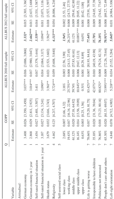
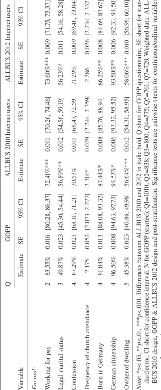
We start with the results of the first step of the investigation of mode systems: the direct comparison without any adjustment for differences in coverage. Table 2 presents the estimates obtained from each survey and the results of the tests for statistical significance of the differences. The online GOPP differs from the ALL-BUS face-to-face reference surveys in both attitudinal and factual questions. We find statistically significant differences between GOPP and ALLBUS 2010 on 11 out of 12 attitudinal items. The only variable for which no differences are found is the respondent’s self-rated financial situation. GOPP differs from ALLBUS 2012 on all attitudinal variables, with the exception of 3 items from the anomie-battery, that is, the differences are found on 9 out of 12 attitudinal variables. For factual questions, GOPP differs from the two ALLBUS surveys on all 7 items at a statisti-cally significant level. When we compare the two ALLBUS surveys, we find dif-ferences for 10 out of 12 attitudinal variables: current and prospective state of the German economy, current self-rated financial situation, religiosity, the items of the anomie-battery, left-right orientation, and self-assessed social class. For the factual questions, no significant differences between the two ALLBUS surveys were found.

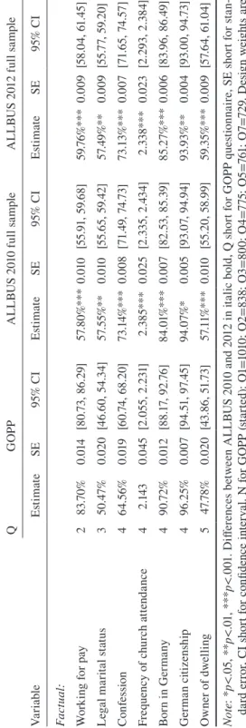
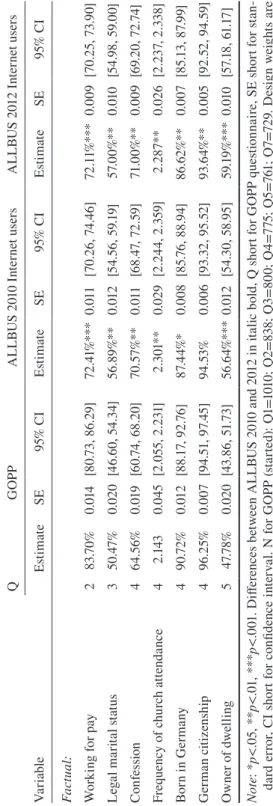
In the next step, we investigate the effect of coverage bias. Table 3 presents the results of the comparisons between the online GOPP with subsamples of Internet users from the two ALLBUS surveys, excluding the non-Internet-users in ALLBUS from the analysis. For several attitudinal variables that showed statistically signifi-cant differences between GOPP and the two ALLBUS surveys, no differences are found when GOPP is compared to ALLBUS Internet users only. The difference with the results of the first step indicates potential coverage bias when measur-ing attitude questions online. For Internet users only, GOPP and ALLBUS 2010 only differ on 6 instead of 11 out of 12 attitudinal items: current and prospective state of German economy, health status, religiosity, one item of the anomie-battery,

and left-right orientation. The differences from the subsample of Internet users in ALLBUS 2012 are found for 4 instead of 9 attitudinal variables: prospective Ger-man economy, current self-rated financial situation, religiosity, and one category of the variable self-assessed social class. We find statistically significant differences between GOPP and the subsample of Internet users in ALLBUS 2010 for all factual variables with the exception of the variable “German citizenship.” The differences between GOPP and ALLBUS 2012 Internet users are statistically significant for all 7 factual variables. With the exception of prospective financial situation and self-assessed social class, the ALLBUS surveys differ from one another on all attitudi-nal variables. In sum, when comparing the subsamples of Internet users, ALLBUS surveys differ from each other in 10 out of 12 attitudinal variables and none of the factual variables.

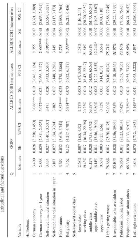
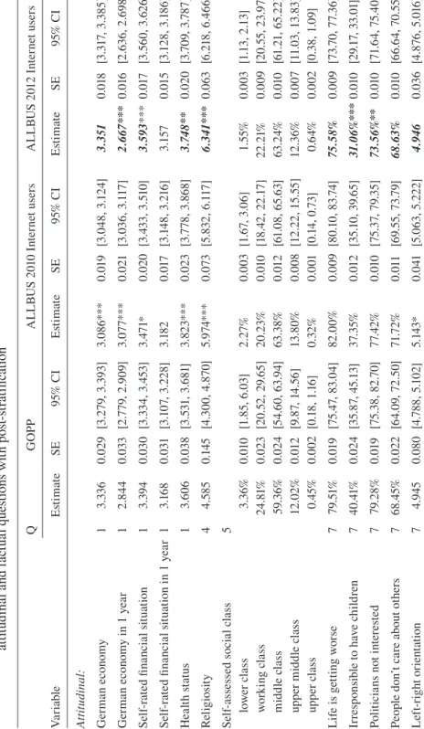
In the last step, we use weighting adjustment to compensate for potential dif-ferences in nonresponse between the surveys. Table 4 reports all comparisons using weighted data. The set of variables in which the online GOPP differs from the ALLBUS surveys is different from the set of variables that showed significant dif-ferences reported in Table 3, where sample composition bias due to coverage but not due to nonresponse was taken into account. The online GOPP now differs from both ALLBUS surveys in 6 out of 12 attitudinal items. In the following, we refer to the comparisons of GOPP with the subsamples of Internet users in ALLBUS with post-stratification weighting applied to GOPP and to ALLBUS 2012.

The variables in which GOPP differs from ALLBUS 2010 are not the same variables in which GOPP differs from ALLBUS 2012. Significant differences between ALLBUS 2010 and GOPP are now observed for the following attitudi-nal variables: state of German economy (both current and prospective), self-rated current financial situation, health status, religiosity, and left-right orientation. The set of attitudinal variables with statistically significant differences between GOPP and ALLBUS 2012 excludes the current state of German economy and left-right orientation, but includes two of the items of the anomie-battery. However, the two ALLBUS surveys still show significant mutual differences for the same 10 out of 12 items reported in Table 3.

Ta bl e 2 Co m pa ris on o f t he G ES IS O nl in e P an el P ilo t t o t wo A LL BU S s ur ve ys : at tit ud in al a nd f ac tu al q ue sti on s Q G OPP A LL BU S 2 01 0 f ul l s am pl e A LL BU S 2 01 2 f ul l s am pl e Va ria bl e Es tima te SE 95% C I Es tima te SE 95% C I Es tima te SE 95% C I At tit ud in al : G er m an e con om y 1 3. 40 0 0.0 26 [3. 35 0, 3. 45 0] 3. 03 7*** 0.0 16 [3. 00 6, 3. 06 8] 3. 33 2* 0.0 15 [3. 30 3, 3. 36 0] G er m an e con om y i

n 1 y

ea r 1 2.8 68 0.0 29 [2. 81 1, 2. 92 5] 3. 01 4*** 0.0 17 [2 .9 80 , 3 .0 47 ] 2. 66 2*** 0.0 13 [2 .6 37 , 2 .6 88 ] Se lf-ra te d fi na nc ia l s itu at ion 1 3. 45 4 0.0 27 [3. 40 1, 3. 50 7] 3. 411 0.0 17 [3. 37 9, 3. 44 4] 3. 55 9 ** 0.0 14 [3. 53 1, 3. 58 7] Se lf-ra te d fi na nc ia l s itu at ion i

n 1 y

Q G OPP A LL BU S 2 01 0 f ul l s am pl e A LL BU S 2 01 2 f ul l s am pl e Va ria bl e Es tima te SE 95% C I Es tima te SE 95% C I Es tima te SE 95% C I Fa ct ua l: W or ki ng for pa y 2 83 .70 % 0.0 14 [8 0.7 3, 86. 29 ] 57 .8 0% *** 0.0 10 [55. 91 , 5 9.6 8] 59 .76 %*** 0.0 09 [58 .0 4, 61 .45 ] Le ga l m ar ita l st at us 3 50 .47% 0.0 20 [46 .60 , 5 4. 34 ] 57. 55 %* * 0.0 10 [55. 65 , 5 9.4 2] 57. 49 %* * 0.0 09 [55. 77 , 5 9.2 0] Con fe ss ion 4 64 .5 6% 0.0 19 [6 0.7 4, 68 .2 0] 73 .14 %*** 0.0 08 [7 1.49 , 7 4.73 ] 73 .13 %*** 0.0 07 [7 1.65 , 7 4. 57 ] Fr eq ue nc y o f c hu rc h a tte nd anc e 4 2. 14 3 0.0 45 [2 .05 5, 2 .2 31 ] 2. 38 5*** 0.0 25 [2. 33 5, 2. 43 4] 2. 33 8*** 0.0 23 [2. 29 3, 2. 38 4] Bo rn i n G er m an y 4 90 .72 % 0.0 12 [88. 17 , 9 2.7 6] 84 .01 %*** 0.0 07 [8 2. 53 , 8 5. 39 ] 85. 27% ** * 0.0 06 [8 3.9 6, 86. 49 ] G er m an cit iz en sh ip 4 96 .2 5% 0.0 07 [9 4. 51 , 9 7.4 5] 94 .0 7%* 0.0 05 [9 3. 07 , 9 4.9 4] 93 .93 %* * 0.0 04 [9 3. 00 , 9 4.7 3] O w ne r o f d we lli ng 5 47 .78% 0.0 20 [4 3. 86 , 5 1.7 3] 57 .11 %*** 0.0 10 [55. 20 , 5 8. 99 ] 59 .3 5% *** 0.0 09 [5 7.6 4, 61 .0 4] No te : * p <. 05 , * * p <. 01 , *** p <. 00 1. D iff er enc es b et we en A LL BU S 2 01 0 a nd 2 01 2 i n i ta lic b ol

d, Q s

ho rt f or G O PP q ue sti on na ire , S E s ho rt f or s ta n-da rd er ro r, CI sh or t f or con fid enc e in te rv al

. N f

or G O PP (st ar te d) : Q 1= 10 10 ; Q 2= 83 8; Q 3= 80 0; Q 4= 77 5; Q 5= 76 1; Q 7= 72 9. D es ig n we ig ht s a re ap pl ie d t o a ll t hr ee s ur ve ys . S ig ni fic anc e t es ts a re p ai rw ise t -te sts f or c on tin uo us /o rd in al v ar ia bl es o r t es ts o f p ro po rti on s. Ta bl

e 2 c

on

tinu

Ta bl e 3 Co m pa ris on o f t he G ES IS O nl in e P an el P ilo t t o t he s ubs am pl es o f I nt er ne t u se rs f ro m t wo A LL BU S s ur ve ys : at tit ud in al a nd f ac tu al q ue sti on s Q G OPP A LL BU S 2 01 0 I nt er ne t user s A LL BU S 2 01 2 I nt er ne t user s Va ria bl e Es tima te SE 95% C I Es tima te SE 95% C I Es tima te SE 95% C I At tit ud in al : G er m an e con om y 1 3. 40 0 0.0 26 [3. 35 0, 3. 45 0] 3. 08 6*** 0.0 19 [3. 04 8, 3. 12 4] 3. 35 5 0.0 17 [3. 32 1, 3. 38 9] G er m an e con om y i

n 1 y

ea r 1 2.8 68 0.0 29 [2. 81 1, 2. 92 5] 3. 07 7*** 0.0 21 [3. 03 6, 3. 11 7] 2. 66 3*** 0.0 15 [2 .6 33 , 2 .6 94 ] Se lf-ra te d fi na nc ia l s itu at ion 1 3. 45 4 0.0 27 [3. 40 1, 3. 50 7] 3. 471 0.0 20 [3. 43 3, 3. 51 0] 3. 59 5 *** 0.0 16 [3. 56 4, 3. 62 7] Se lf-ra te d fi na nc ia l s itu at ion i

n 1 y

Q G OPP A LL BU S 2 01 0 I nt er ne t user s A LL BU S 2 01 2 I nt er ne t user s Va ria bl e Es tima te SE 95% C I Es tima te SE 95% C I Es tima te SE 95% C I Fa ct ua l: W or ki ng for pa y 2 83 .70 % 0.0 14 [8 0.7 3, 86. 29 ] 72 .41 %*** 0.0 11 [7 0. 26 , 7 4.4 6] 72 .11 %*** 0.0 09 [7 0. 25, 7 3.9 0] Le ga l m ar ita l st at us 3 50 .47% 0.0 20 [46 .60 , 5 4. 34 ] 56 .8 9% ** 0.0 12 [5 4. 56 , 5 9.1 9] 57. 00 %* * 0.0 10 [5 4. 98 , 5 9.0 0] Con fe ss ion 4 64 .5 6% 0.0 19 [6 0.7 4, 68 .2 0] 70 .5 7%* * 0.0 11 [68 .47 , 7 2. 59 ] 71 .0 0%* * 0.0 09 [6 9.2 0, 7 2.7 4] Fr eq ue nc y o f c hu rc h a tte nd anc e 4 2. 14 3 0.0 45 [2 .05 5, 2 .2 31 ] 2. 30 1* * 0.0 29 [2. 24 4, 2. 35 9] 2.2 87 ** 0.0 26 [2 .2 37 , 2 .33 8] Bo rn i n G er m an y 4 90 .72 % 0.0 12 [88. 17 , 9 2.7 6] 87. 44 %* 0.0 08 [8 5.7 6, 88. 94 ] 86. 62 %* * 0.0 07 [8 5.1 3, 8 7.9 9] G er m an cit iz en sh ip 4 96 .2 5% 0.0 07 [9 4. 51 , 9 7.4 5] 94 .53% 0.0 06 [9 3. 32 , 9 5. 52] 93 .6 4%* * 0.0 05 [92 .5 2, 94 .5 9] O w ne r o f d we lli ng 5 47 .78% 0.0 20 [4 3. 86 , 5 1.7 3] 56 .6 4% *** 0.0 12 [5 4. 30 , 5 8. 95 ] 59 .19 %*** 0.0 10 [5 7.1 8, 61 .17 ] No te : * p <. 05 , * * p <. 01 , *** p <. 00 1. D iff er enc es b et we en A LL BU S 2 01 0 a nd 2 01 2 i n i ta lic b ol

d, Q s

ho rt f or G O PP q ue sti on na ire , S E s ho rt f or s ta n-da rd er ro r, CI sh or t f or con fid enc e in te rv al

. N f

or G O PP (st ar te d) : Q 1= 10 10 ; Q 2= 83 8; Q 3= 80 0; Q 4= 77 5; Q 5= 76 1; Q 7= 72 9. D es ig n we ig ht s a re ap pl ie d t o a ll t hr ee s ur ve ys . S ig ni fic anc e t es ts a re p ai rw ise t -te sts f or c on tin uo us /o rd in al v ar ia bl es o r t es ts o f p ro po rti on s. Ta bl

e 3 c

on

tinu

Ta bl e 4 Co m pa ris on o f t he G ES IS O nl in e P an el P ilo t t o t he s ubs am pl es o f I nt er ne t u se rs f ro m t wo A LL BU S s ur ve ys : at tit ud in al a nd f ac tu al q ue sti on s w ith p os t-s trat ifi cat io n Q G OPP A LL BU S 2 01 0 I nt er ne t user s A LL BU S 2 01 2 I nt er ne t user s Va ria bl e Es tima te SE 95% C I Es tima te SE 95% C I Es tima te SE 95% C I At tit ud in al : G er m an e con om y 1 3. 33 6 0.0 29 [3. 27 9, 3. 39 3] 3. 08 6*** 0.0 19 [3. 04 8, 3. 12 4] 3. 351 0.0 18 [3. 31 7, 3. 38 5] G er m an e con om y i

n 1 y

ea r 1 2.8 44 0.0 33 [2. 77 9, 2. 90 9] 3. 07 7*** 0.0 21 [3. 03 6, 3. 11 7] 2. 66 7*** 0.0 16 [2 .6 36 , 2 .6 98 ] Se lf-ra te d fi na nc ia l s itu at ion 1 3. 39 4 0.0 30 [3. 33 4, 3. 45 3] 3. 47 1* 0.0 20 [3. 43 3, 3. 51 0] 3. 593 *** 0.0 17 [3. 56 0, 3. 62 6] Se lf-ra te d fi na nc ia l s itu at ion i

n 1 y

Q G OPP A LL BU S 2 01 0 I nt er ne t user s A LL BU S 2 01 2 I nt er ne t user s Va ria bl e Es tima te SE 95% C I Es tima te SE 95% C I Es tima te SE 95% C I Fa ct ua l: W or ki ng for pa y 2 83 .5 5% 0.0 16 [8 0. 28 , 86. 37 ] 72 .41 %*** 0.0 11 [7 0. 26 , 7 4.4 6] 73 .6 0% *** 0.0 09 [7 1.75 , 75 .3 7] Le ga l m ar ita l st at us 3 49. 87 % 0.0 23 [4 5. 30 , 5 4.4 4] 56 .8 9% ** 0.0 12 [5 4. 56 , 5 9.1 9] 56 .2 3%* 0.0 11 [5 4.16 , 5 8. 28 ] Con fe ss ion 4 67. 29 % 0.0 21 [6 3.10 , 7 1.21 ] 70 .5 7% 0.0 11 [68 .47 , 7 2. 59 ] 71. 29 % 0.0 09 [6 9.4 6, 7 3. 04 ] Fr eq ue nc y o f c hu rc h a tte nd anc e 4 2. 17 5 0.0 52 [2. 07 3, 2. 27 7] 2. 30 1* 0.0 29 [2. 24 4, 2. 35 9] 2. 286 0.0 26 [2 .23 4, 2 .3 37 ] Bo rn i n G er m an y 4 91 .0 4% 0.0 13 [88. 08 , 9 3. 32 ] 87. 44 %* 0.0 08 [8 5.7 6, 88. 94 ] 86. 25 %* * 0.0 08 [8 4.6 9, 8 7.6 7] G er m an cit iz en sh ip 4 96 .50 % 0.0 08 [9 4. 63 , 9 7.7 3] 94 .53% * 0.0 06 [9 3. 32 , 9 5. 52] 93 .50 %* * 0.0 06 [92 .3 3, 94 .5 0] O w ne r o f d we lli ng 5 45. 38 % 0.0 23 [4 0. 86 , 4 9.9 8] 56 .6 4% *** 0.0 12 [5 4. 30 , 5 8. 95 ] 58 .0 6% *** 0.0 10 [5 6. 99 , 6 0.1 0] No te : * p <. 05 , * * p <. 01 , *** p <. 00 1. D iff er enc es b et we en A LL BU S 2 01 0 a nd 2 01 2 i n i ta lic b ol

d, Q s

ho rt f or G O PP q ue sti on na ire , S E s ho rt f or s ta n-da rd e rro r, C I s ho rt f or c on fid enc e i nt er va

l. N f

or G O PP ( sta rte d) : Q 1= 10 10 ; Q 2= 83 8; Q 3= 80 0; Q 4= 77 5; Q 5= 76 1; Q 7= 72 9. W eig ht ed d at a: A LL -BU S 2 01 0 d es ig n, G O

PP & A

LL BU S 2 01 2 d es ig n a nd p os t-s tra tifi ca tion. S ig ni fic anc e t es ts a re p ai rw ise t -te sts f or c on tin uo us /o rd in al v ar ia bl es or t es ts o f p ro po rti on s. Ta bl

e 4 c

on

tinu

The fact that the two face-to-face ALLBUS surveys differ on attitudinal ques-tions shows that attitudes, being more unstable constructs, would not have allowed us to single out a mode system effect. We see that two surveys with identical recruit-ment and design features do not differ in factual questions, whereas the difference between the online and the face-to-face surveys is clear.

However, finding statistically significant differences is not the only indicator of mode system effects. In addition to statistical significance, Biemer (1988) recom-mends examining the effect size, the direction of the difference, and the violations of the underlying assumptions for the mode comparison study, which could explain the magnitude of the difference.

Calculating effect sizes standardizes the comparisons between the means and proportions reported in Table 4 and allows for a better estimation of error, because effect sizes do not only take the difference of the estimates into account, but also the sample sizes and the precision of estimates.

We calculated the standardized mean difference effect sizes that are used to synthesize results from studies that contrast two groups on measures with a contin-uous underlying distribution for the continous and ordinal variables (Lipsey & Wil-son, 2001, p. 172) and approximated standardized mean difference effect sizes that are calculated differencing the arcsine-transformed proportions (Lipsey & Wilson, 2001, p. 187) for binary variables.15 _{The standardized mean difference effect sizes} allow us to compare the size and direction of the difference between the GOPP and ALLBUS 2010 with the difference between GOPP and ALLBUS 2012 as well as with the difference between ALLBUS 2010 and ALLBUS 2012 for each variable. In order to compare the differences between the surveys for groups of variables (attitudinal vs. factual), we calculated the mean effect sizes. The mean effect size is computed by weighting each effect size by the inverse of its variance (Lipsey & Wilson, 2001, p. 114). Since the standardized mean effect sizes take the direction of the difference (indicated by the sign of the effect size) into account, the differ-ences between the variables may be underestimated when the sum of the negative

15 The standardized mean difference effect size (ESsm) is the difference between the group means (X) divided by the pooled standard deviation (s), which is calculated based on the sample sizes for each group:

1 2

sm

pooled

X X

ES s

−

= , 1 12 2 22

1 2

( 1) ( 1)

2

pooled n s n s

s

n n

− + −

=

+ − .

The approximations based on dichotomous data: ES =arcsine psm ( )1 −arcsine p( )2,

where p is the proportion for each group (Lipsey & Wilson, 2001, p. 198-200). The mean effect size 1

2 1

( )_; 1

k

i i

i

i k

i

i i

w ES

ES w

w _SE

= =

×

=∑ =

∑ ,

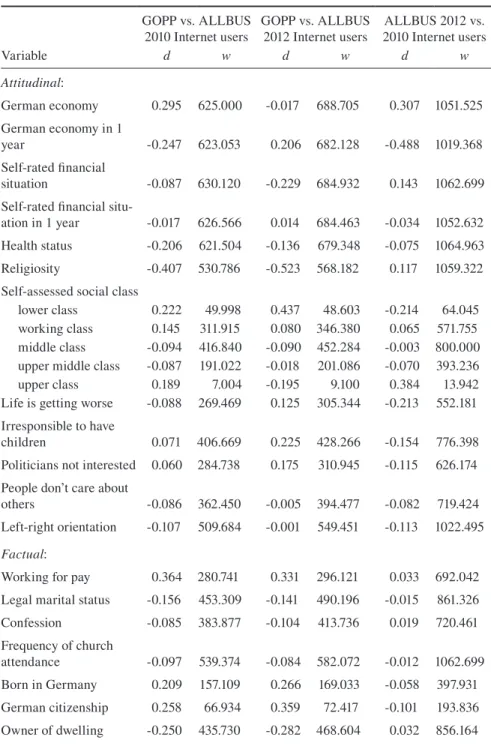
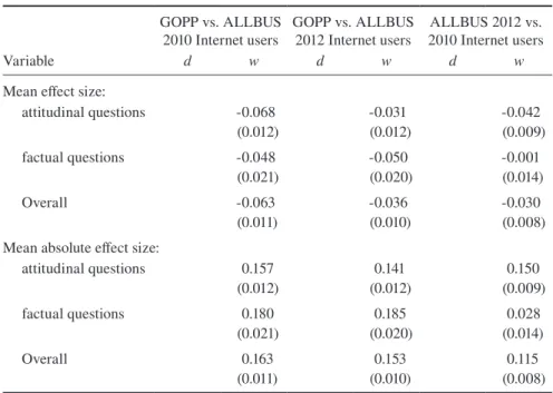
and positive effect sizes is calculated in order to compute the mean effect size. We therefore also calculate the absolute mean effect sizes, which are based on abso-lute values of the standardized mean difference effect sizes. In Table 5, we report the standardized mean difference effect sizes (d) and mean effect sizes as well as absolute mean effect sizes for attitudinal variables, factual variables and the overall mean effect size, which incorporates both attitudinal and factual variables.

From Table 5, we can conclude that the directions of all mean effect sizes are the same. For weighted mean effect sizes over all questions, the difference between GOPP and ALLBUS 2010 (-0.063) and the difference between GOPP and ALLBUS 2012 (-0.036) are larger than the difference between the two ALLBUS surveys (-0.030). However, the difference between GOPP and ALLBUS 2012 has almost the same magnitude as the difference between the two face-to-face reference surveys.

Table 5 Effect sizes (d), inverse variance weights (w) and mean effect sizes across the surveys

Variable

GOPP vs. ALLBUS

2010 Internet users GOPP vs. ALLBUS 2012 Internet users 2010 Internet usersALLBUS 2012 vs.

d w d w d w

Attitudinal:

German economy 0.295 625.000 -0.017 688.705 0.307 1051.525 German economy in 1

year -0.247 623.053 0.206 682.128 -0.488 1019.368

Self-rated financial

situation -0.087 630.120 -0.229 684.932 0.143 1062.699 Self-rated financial

situ-ation in 1 year -0.017 626.566 0.014 684.463 -0.034 1052.632 Health status -0.206 621.504 -0.136 679.348 -0.075 1064.963 Religiosity -0.407 530.786 -0.523 568.182 0.117 1059.322 Self-assessed social class

lower class 0.222 49.998 0.437 48.603 -0.214 64.045 working class 0.145 311.915 0.080 346.380 0.065 571.755 middle class -0.094 416.840 -0.090 452.284 -0.003 800.000 upper middle class -0.087 191.022 -0.018 201.086 -0.070 393.236

upper class 0.189 7.004 -0.195 9.100 0.384 13.942

Life is getting worse -0.088 269.469 0.125 305.344 -0.213 552.181 Irresponsible to have

children 0.071 406.669 0.225 428.266 -0.154 776.398 Politicians not interested 0.060 284.738 0.175 310.945 -0.115 626.174 People don’t care about

others -0.086 362.450 -0.005 394.477 -0.082 719.424 Left-right orientation -0.107 509.684 -0.001 549.451 -0.113 1022.495 Factual:

Working for pay 0.364 280.741 0.331 296.121 0.033 692.042 Legal marital status -0.156 453.309 -0.141 490.196 -0.015 861.326 Confession -0.085 383.877 -0.104 413.736 0.019 720.461 Frequency of church

Variable

GOPP vs. ALLBUS

2010 Internet users GOPP vs. ALLBUS 2012 Internet users 2010 Internet usersALLBUS 2012 vs.

d w d w d w

Mean effect size:

attitudinal questions -0.068

(0.012) -0.031(0.012) -0.042(0.009)

factual questions -0.048

(0.021) -0.050(0.020) -0.001(0.014)

Overall -0.063

(0.011) -0.036(0.010) -0.030(0.008) Mean absolute effect size:

attitudinal questions 0.157

(0.012) (0.012)0.141 (0.009)0.150

factual questions 0.180

(0.021) (0.020)0.185 (0.014)0.028

Overall 0.163

(0.011) (0.010)0.153 (0.008)0.115 Note: d is the unweighted effect size, w is the inverse variance weight, standard errors in

parentheses.

6 Discussion

We investigated mode system effects by comparing the data from a probability-based telephone-recruited online panel with the data from two face-to-face surveys. All three sources implemented questions with identical wording and we controlled for differences in sample composition due to undercoverage and selective nonre-sponse in order to single out the mode system effect. We distinguished between factual and attitudinal questions. We hypothesized that the effects are more pro-nounced for attitudinal questions than for factual questions. This hypothesis finds no support. There are differences between the online collected data and interviewer collected data on both types of questions. However, the distinction between factual and attitudinal data remains important. We did find that for factual questions both face-to-face surveys differ from the online panel, but do not differ significantly from each other. This conclusion is supported by the analysis of effect sizes. For attitudi-nal questions, the difference between the two interviewer-administered face-to-face surveys is larger than the difference between one face-to-face survey (ALLBUS 2012) and the online panel. We attribute this result to the instability of attitudes. However, alternative explanations are possible. For example, the reference period

of the ALLBUS 2012 is closer to the online panel, which was administered in 2011-2012 than to the ALLBUS 2010. Surprisingly, the mean effect size for differences in attitudinal variables is larger for ALLBUS 2010 to ALLBUS 2012 comparison than for the GOPP to ALLBUS 2012 comparison, although all effect sizes are small. When we look at the content of the questions, we see that effect sizes are relatively large for questions that refer to the economic situation. The differences between the surveys on those variables might be attributed not to the mode system effect, but to the fact that Germany experienced real economic changes between 2010 and 2012. To examine the robustness of our results, we recalculated what the effect sizes are when the four variables that refer to the economic condition are excluded. This did not affect our overall conclusions, but it provided us with more accurate measures of the mode system effect.16

When comparing data from surveys to data from benchmark studies, Calle-garo et al. (2014) advise that the following conditions be met: (1) question word-ing should be identical across compared surveys and (2) populations represented by each survey need to be comparable. Typically, studies comparing online panel data to benchmarks use demographic and behavioral measures (Callegaro et al., 2014). One of the reasons for this might be that the official statistics ideally used as benchmarks can only provide such data. If benchmarks come from high-quality surveys, using attitudinal measures can be considered. Our study meets both condi-tions (identical quescondi-tions wording and comparable populacondi-tions after adjustment) and shows the importance of the reference period depending on the nature of the measure. Ideally, the reference period should be the same for a benchmark source (survey) and the survey that is being compared to the benchmark – a situation given when a pure mode effect is estimated in a randomized experiment. However, in practical circumstances – when estimating a mode system effect – this might not be the case.

Our findings have important implications for estimating mode system effects. First, we have shown the importance of having more than one reference survey. In our case, both face-to-face surveys serve as control surveys for the online panel and allow us to draw conclusions about whether or not differences could be attributed to the mode. We use two surveys with equal recruitment procedures. Second, we show the importance of distinguishing between types of questions. In past studies, dif-ferences between online and interviewer-administered modes are well-documented for sensitive questions (e.g., meta-analysis by Tourangeau, Conrad, & Couper, 2013,

p. 142).17 _{We draw on another dimension, in which a distinction is made based on} the cognitive demands that questions place on a respondent. Our findings are in line with Klausch, Hox, and Schouten (2014), who also report that mode effects depend on the question type. For data analysts, the conclusion to be drawn from our analy-sis is that mode system effects differ across question types. Data users should there-fore have different concerns about mode effects when analyzing only attitudinal, only factual, or both types of items. Third, we find a common denominator for the comparison of mode system effects by reporting effect sizes. The magnitude of the mode system effect when judged by the effect sizes is small. However, researchers who use data from large surveys might be misled if they rely solely on significance testing. We encourage other researchers to report effect sizes. This would allow for comparing our results to similar studies based on different data. Fourth, it is important to realize, that we corrected for sample composition bias, and found indi-cations of coverage and nonresponse bias. In survey practice, one could use mixed-mode approaches to account for the digital divide; an example is the GESIS Panel18_, where a mix of postal mail and Internet is used for data collection.

Finally, we investigated the effect of mode systems on point estimates answer-ing the practical question of survey practitioners, of what happens when we change our data collection procedures. To tease out the reasons for mode system effects, a series of carefully designed experiments is needed. These experiments should take both selection and measurement effects into account and not only use point estimates, but also rely on other indicators, such as indices for response tendencies (cf. Tourangeau, 2013).

17 We did not have sensitive items to use for our analysis. However, for religiosity, we find that the percentage online panel respondents who choose the answer “not religious” is much higher than for interviewer-administered surveys (29.44% with SE=0.021, CI=[25.56, 33.64] for GOPP and 7.72% with SE=0.007, CI=[6.54, 9.10] for ALLBUS 2010, 6.27% with SE=0.005, CI=[5.32, 7.38], p<.001 for GOPP vs. either ALLBUS). This could be indicative of social desirability.

References

American Association for Public Opinion Research. (2011). Standard Definitions: Final Dis-positions of Case Codes and Outcome Rates for Surveys. 7th _{edition: AAPOR.}

Auspurg, K., Burton, J., Cullinane, C., Delavande, A., Fumagelli, L., Iacovou, M., Zafar, B. (2013). Understanding Society Innovation Panel Wave 5: Results from Methodological Experiments. In J. Burton (Ed.), Understanding Society Working Paper Series. Essex: Institute for Social and Economic Research, University of Essex.

Bandilla, W., Kaczmirek, L., Blohm, M., & Neubarth, W. (2009). Coverage und Nonres-ponse-Effekte bei Online-Bevölkerungsumfragen [Coverage and nonresponse effects in online population-surveys]. In N. Jackob, H. Schoen & T. Zerback (Eds.), Sozial-forschung im Internet: Methodologie und Praxis der Online-Befragung (pp. 129-143). Wiesbaden: VS Verlag.

Bergmann, M. (2011). Stata-ado “ipfweight”: IPF-Algorithm to create adjustment survey weights. from http://fmwww.bc.edu/repec/bocode/i/ipfweight.ado

Biemer, P. P. (1988). Measuring Data Quality. In R. M. Groves, P. P. Biemer, L. E. Lyberg, J. T. Massey, W. L. Nicholls & J. Waksberg (Eds.), Telephone Survey Methodology (pp. 273-283). New York: Wiley.

Biemer, P. P., & Lyberg, L. E. (2003). Introduction to survey quality. Hoboken, New Jersey: Wiley.

Bosnjak, M., Haas, I., Galesic, M., Kaczmirek, L., Bandilla, W., & Couper, M. P. (2013). Sample composition discrepancies in different stages of a probability-based online pa-nel. Field Methods. doi: 10.1177/1525822X12472951

Callegaro, M., Villar, A., Yeager, D., & Krosnick, J. A. (2014). A critical review of studies investigating the quality of data obtained with online panels based on probability and nonprobability samples. In M. Callegaro, R. Baker, J. D. Bethlehem, A. S. Göritz, J. A. Krosnick & P. J. Lavrakas (Eds.), Online panel research: A data quality perspective (pp. 23-53). New York: Wiley.

Couper, M. P. (2011). The future of modes of data collection. Public Opinion Quarterly, 75, 5, 889-908.

Couper, M. P., Kapteyn, A., Schonlau, M., & Winter, J. (2007). Noncoverage and Nonres-ponse in an Internet Survey. Social Science Research, 36, 131-148.

Dehming, W. E., & Stephan, F. F. (1940). On a least squares adjustment of a sampled fre-quency table when the expected marginal totals are known. The Annals of Mathemati-cal Statistics, 11(4), 427-444.

de Leeuw, E. D. (1992). Data quality in mail, telephone, and face-to-face surveys. Amster-dam: TT.Publikaties. http://edithl.home.xs4all.nl/pubs/disseddl.pdf

de Leeuw, E. D. (2005). To Mix or Not to Mix Data Collection Modes in Surveys. Journal of Official Statistics, 21(2), 233-255.

de Leeuw, E. D., & Hox, J. J. (2011). Internet surveys as a part of a mixed-mode design. In M. Das, P. Ester & L. Kaczmirek (Eds.), Social and behavioral research and the Inter-net (Vol. 45-76). New York: Routledge.

Ferguson, C. J. (2009). An Effect Size Primer: A Guide for Clinicians and Researchers. Professional Psychology: Research and Practice, 40(5), 532–538.

Hoffmeyer-Zlotnik & D. Krebs (Eds.), Gewichtung in der Umfragepraxis [Weighting in the Survey Practice] (pp. 88-105). Westdeutscher Verlag

Gabler, S., & Ganninger, M. (2010). Gewichtung [Weighting]. In C. Wolf & H. Best (Eds.), Handbuch der sozialwissenschaftlichen Datenanalyse [Handbook of the Data Analy-ses in the Social Sciences] (pp. 143-164). Wiesbaden: VS Verlag.

Gabler, S., & Häder, S. (2002). Telefonstichproben. Methodische Innovationen und Anwen-dungen in Deutschland [Telephone samples: Methodological innovations and applica-tions in Germany]. Münster: Waxmann Verlag.

Gabler, S., Häder, S., Lehnhoff, I. & Mardian, E. (2012). Weighting for unequal inclusion probabilities and nonresponse in dual frame telephone surveys. In S. Häder, M. Häder & M. Kühne (Eds.), Telephone surveys in Europe: Research and practice (pp. 147-167). Heidelberg: Springer.

Groves, R. M. (1989). Survey errors and survey costs. New York: Wiley.

Groves, R. M. & Couper, M. P. (1998). Nonresponse in household interview surveys. New York: Wiley.

Groves, R. M., Fowler, F. J., Couper, M. P., Lepkowski, J. M., Singer, E., & Tourangeau, R. (2009). Survey methodology (2nd ed.). New York: John Wiley.

Hox, J. J., de Leeuw, E. D., & Zijlmans, E. A. O. (2015). Measurement equivalence in mixed-mode surveys. Frontiers in Psychology, 6(87). doi: 10.3389/fpsyg.2015.00087

Klausch, T., Hox, J. J., & Schouten, B. (2013). Measurement effects of survey mode on the equivalence of attitudinal rating scale questions. Sociological Methods & Research 42(3), 227-263.

Klausch, T., Hox, J. J., & Schouten, B. (2014). Evaluating mixed-mode redesign strategies against benchmark surveys: The case of the Crime Victimization Survey. Paper presen-ted at the GOR General Online Conference, 05-07.03.2014 in Cologne.

Lee, S. (2006). An Evaluation of Nonresponse and Coverage Errors in a Prerecruited Proba-bility Web Panel Survey. Social Science Computer Review, 24, 460-475.

Lipsey, M. W., & Wilson, D. B. (2001). Practical meta-analysis. Thousand Oaks, Califor-nia: Sage.

Little, R. J. A., & Wu, M. (1991). Models for contingency tables with known margins when target and sampled populations differ. Journal of the American Statistical Association, 86(413), 87-95.

Lois, D. (2011). Kirchenmitgliedschaft und Kirchgangshäufigkeit im Zeitverlauf

– Eine Trendanalyse unter Berücksichtigung von Ost-West-Unterschieden [Church membership and frequency of church attendance over time – A trend analysis taking into consideration differences in East and West Germany]. Comparative Population Studies – Zeitschrift für Bevölkerungswissenschaft, 36(1), 127-160.

Lyberg, L., & Kasprzyk, D. (1991). Data collection methods and measurement error: An overview. In P. P. Biemer, R. M. Groves, L. E. Lyberg, N. A. Mathiowetz, & S. Sudman (Eds.), Measurement errors in surveys (pp. 237-257). New York: Wiley.

Mohorko, A., de Leeuw, E., & Hox, J. (2013). Journal of Officila Statistics, 29, 4, 609-622. http://www.degruyter.com/view/j/jos.2013.29.issue-4/jos-2013-0042/jos-2013-0042. xml

Schouten, B., Van den Brakel, J., Buelens, B., & Klausch, T. (2013). Disentangling mode-specific selection and measurement bias in social surveys. Social Science Research, 42, 1555-1570.

Tourangeau, R. (2013). Confronting the challenges of household surveys by mixing modes. Keynote address at the 2013 Federal Committee on Statistical Methodology Research Conference, Nov 4, 2013, Washington DC. http://www.copafs.org/UserFiles/file/fcsm/ Tourangeau2013FCSMResearchKeynote.pdf

Tourangeau, R., Conrad, F. G., & Couper, M. P. (2013). The science of web surveys. Oxford: Oxford University Press.

Tourangeau, R., Rips, L. J., & Rasinski, K. (2000). The psychology of survey response. Cambridge: Cambridge University Press.

Appendix

-5 & 7

A LL BU S 2 01 0 I nt er ne t user s A LL BU S 2 01 2 I nt er ne t user s Va ria bl e % SE CI % SE CI % SE CI M ale 53 .1 .01 5 [5 0.1 , 5 6.0 ] 51 .5 .01 2 [4 9.3 , 5 3. 8] 51 .6 .010 [4 6. 4, 5 0. 3] A ge g ro up s 18 -2 4 13 .0 .010 [1 1.2 , 1 5.1] 13 .9 .0 08 [1 2. 4, 1 5.6 ] 13 .9 .0 07 [1 2. 6, 1 5. 3] 25 -34 19. 8 .01 2 [1 7.6 , 2 2. 3] 18 .6 .0 09 [16 .9, 2 0. 4] 17. 4 .0 08 [1 5.9 , 1 8.9 ] 35 -4 9 34 .9 .014 [3 2. 2, 3 7.8 ] 35. 4 .011 [3 3. 2, 3 7.6 ] 31 .4 a .0 09 [2 9.6 , 3 3. 3] 50 -6 4 23. 4 .01 3 [2 1.0 , 2 6.0 ] 23. 2 .010 [21 .4 , 2 5. 2] 27. 7 a .0 09 [2 6. 0, 2 9.5 ] 65+ 8.8 .0 08 [7 .3 , 1 0.6 ] 8.9 .0 07 [7 .6 , 1 0. 2] 9.6 .0 06 [8 .5, 10 .9] Ed uc at io n lo w 12 .5 .010 [1 0.7 , 1 4.6 ] 21 .4 .010 [1 9.6 , 2 3. 4] 20 .9 .0 08 [1 9.4 , 2 2. 6] m ed iu m 30.0 .014 [2 7.4 , 3 2.7 ] 37. 8 .011 [3 5.6 , 4 0.0 ] 39. 4 .010 [3 7.5 , 4 1.3 ] hig h 57. 5 .01 5 [5 4. 6, 6 0.4 ] 40. 8 .011 [3 8. 5, 4 3. 0] 39 .7 .010 [3 7.8 , 4 1.6 ]

a si

gn ifi ca nt d iff er enc es ( p <0 .01 ) b et we en A LL BU S 2 01 0 a nd 2 01

2. N f

or G O PP i s 1 11 4 r es pon de nt s, w hi ch i nc lud es t he r es pon de nt s w ho co m pl et ed a t l ea st on e o f t he q ue sti on na ire

s 1 t

Ta bl e A 2 D ist rib ut io ns o f d em og ra ph ic c ha ra ct er ist ics i n t he G O PP o ve r q ue sti on na ire s ( pe rc en ta ge s) Va ria bl e/ Q 1 2 3 4 5 7 M ale 52 .9 7 (. 01 6) [4 9.9 , 5 6.1] 52 .74 (. 017 ) [4 9.4 , 5 6.1] 51 .75 (. 01 8) [4 8. 3, 55. 2] 51 .4 8 (. 01 8) [4 8. 0, 55. 0] 51 .91 (. 01 8) [4 8. 4, 55. 5] 51 .9 9 (. 01 9) [4 8. 4, 55. 6] A ge g ro up s 18 –2 4 13 .3 7 ( .01 1) [11 .4 , 1 5.6 ] 12 .5 3 ( .01 1) [1 0. 5, 1 5.0 ] 12 .12 (. 012 ) [1 0.0 , 1 4.6 ] 12 .5 2 ( .012 ) [1 0. 4, 1 5.0 ] 13 .2

7 (.

01 2) [11 .0 , 1 5.9 ] 12 .3 5 ( .012 ) [1 0.1 , 1 4. 9] 25 –34 19 .31 (. 01 2) [1 7.0 , 2 1.9 ] 19 .21 (. 01 4) [1 6.7 , 22 .0] 19 .2 5 (. 01 4) [1 6.7 , 22 .1] 18 .4 5 (. 01 4) [1 5.9, 21 .3 ] 18 .5 3 (. 01 4) [1 5.9, 21 .5 ] 19 .2 0 (. 01 5) [1 6. 5, 22 .2 ] 35 –4 9 34 .85 (. 01 5) [3 2. 0, 3 7.8 ] 34 .73 (. 01 6) [3 1.6 , 3 8.0 ] 35 .0 0 ( .01 7) [31 .8 , 3 8. 3] 35 .10 (. 017 ) [3 1.8 , 3 8. 5] 34 .0 3 ( .01 7) [3 0.7 , 3 7.5 ] 34 .2 9 (. 01 8) [3 0. 9, 3 7.8 ] 50 –6 4 23 .47 (. 013 ) [2 0. 9, 2 6. 2] 24 .2 2 (. 01 5) [2 1.4 , 2 7.2 ] 24 .5 0 (. 01 5) [2 1.6 , 2 7.6 ] 24 .6 5 ( .01 5) [2 1.7 , 2 7.8 ] 24 .9 7 ( .017 ) [2 2. 0, 2 8.2 ] 24 .9 7 (. 01 6) [2 2. 0, 2 8.2 ] 65+ 9.0 0 ( .0 09 ) [7. 4, 10 .9] 9.3 1 (. 01 0) [7 .5 , 1 1.5 ] 9.1 3 (. 01 0) [7 .3 , 1 1.3 ] 9.2 8 (. 01 0) [7. 4, 11 .6 ] 9.2 0 (. 01 0) [7. 3, 11 .5 ] 9.1 9 ( .01 1) [7. 3, 11 .5 ] Ed uc at io n lo w 12 .18 (. 01 0) [1 0.3 , 1 4.3 ] 11 .81 (. 011 ) [9 .8 , 14 .2 ] 10. 25 (. 01 1) [8. 3, 1 2. 6] 10.0 6 ( .01 1) [8 .1, 1 2. 4] 10. 25 (. 01 1) [8. 3, 1 2. 6] 10.0 1 ( .01 1) [8 .0 , 1 2. 4] m ed iu m 29 .5 0 (. 01 4) [2 6. 8, 3 2. 4] 29 .0 0 ( .01 6) [2 6. 0, 3 2.2 ] 28 .0 0 ( .01 6) [2 5.0, 31 .2 ] 28 .5 2 (. 01 6) [2 5.4, 31 .8 ] 27. 73 (. 01 6) [2 4.7, 31 .0] 27. 57 (. 01 7) [2 4.4 , 3 0. 9] hig h 58 .3 2 (. 01 6) [55. 2, 61 .3 ] 59 .19 (. 017 ) [55. 8, 6 2. 5] 61 .75 (. 01 7) [5 8. 3, 6 5.1] 61 .4 2 ( .01 7) [5 7.9 , 6 4. 8] 62 .0 2 ( .01 8) [5 8. 5, 6 5.4 ] 62 .41 (. 01 8) [5 8. 8, 6 5.9 ] m iss in

g on a

ge 2.0 8 1. 55 1.8 8 1.6 8 1.4 5 1.3 7 m iss in

g on e

du ca tion 8.0 2 3. 34 3. 88 3.7 5 3. 82 3.7 1 m iss in g d es ig n w eig ht 7.1 3 1.91 2.7 5 2.8 4 2. 50 2. 47 N 10 10 838 80 0 775 761 72 9 No te : s ta nd ar d e rro rs i n p ar en th es es , 9 5% -c on fid enc e i nt er va ls i n b ra ck et s. T he d at a a re n ot w eig ht ed

. Q i

Table A3 Post-stratification weights obtained with IPF-Weighting

Questionnaire 1 2 3 4 5 7

N 1010 838 800 775 761 729

Min 0.585 0.539 0.520 0.510 0.507 0.498

Max 2.299 2.367 2.445 3.268 2.956 3.086

1% percentile 0.585 0.539 0.520 0.510 0.507 0.498

99% percentile 2.044 2.137 2.907 2.514 2.528 2.558

Calculation of the effect sizes:

Formulas used for calculating the unweighted effect sizes (Lipsey & Wilson, 2001, p. 172 ff.):

The standardized mean difference effect size (ES_sm):

1 2

sm

pooled

X X

ES s

−

= , 1 12 2 22

1 2

( 1) ( 1)

2

pooled n s n s

s

n n

− + −

=

+ − .

The approximations based on dichotomous data: ES =arcsine psm ( )1 −arcsine p( )2 ,

where p is the proportion for each group (Lipsey & Wilson, 2001, p. 198-200). Formulas used for calculating the mean effect sizes:

1

2 1

( )_; 1

k

i i

i

i k

i

i i

w ES

ES w

w _SE

= =

×

=∑ =

∑ ,

where w is the inverse variance weight, ES is the unweighted effect size (d), and SE

is the standard error of the difference between the effect sizes (Lipsey & Wilson, 2001, p. 114).

For the calculation of the effect sizes the effect size calculator at http://www.camp-bellcollaboration.org/resources/effect_size_input.php was used.

We used the unweighted sample sizes to calculate the mean effects.

Questions used in the analysis

German economy*

How would you generally rate the current economic situation in Germany?

Very good Good

Partly good/partly bad Bad

Very bad

Own financial situation*

And your own current financial situation?

Very good Good

Partly good/partly bad Bad

Very bad

German economy in 1 year*

What do you think the economic situation in Germany will be like in one year?

Considerably better than today Somewhat better than today The same

Somewhat worse than today Considerably worse than today

Own financial situation in 1 year*

And what will your own financial situation be like in one year?

Considerably better than today Somewhat better than today The same

Somewhat worse than today Considerably worse than today

General health*

A question about your health: How would you describe your health in general?

Employment status*

And now let’s continue with employment and your occupation. Which of the cat-egories on the card applies to you?

Full time employment

Part (‘‘half’’) time employment

Less than part (‘‘half’’) time employment Not working

If there are difficulties referring to the classification, here are some hints for you: Trainees are considered employees in a regular occupation.

Family members assisting in a family business who are full- time or part- time (‘‘halftime’’) employees in the business of a household or a family member, without having a formal contract, are also considered employees in a regular occupation (either full- time or part- time).

‘‘Employed less than part- time’’ are persons who are gainfully employed while, at the same time, one of the following applies:

Attend a full- time school (pupils and students), Are registered as unemployed or

Draw a retirement benefit / pension as a result of previous employment.

Persons on maternity / parental leave or on another type of leave of absence are not considered employees in a regular occupation.

Marital status*

What is your marital status? Are you...

Married and living with your spouse Married and living apart

Widowed Divorced Never married

Civil partnership, living together Civil partnership, living apart Registered partner deceased Civil partnership dissolved