Oviedo University Press 116 Economics and Business Letters
6(4), 116-124, 2017
US stocks in the presence of oil price risk:
Large cap vs. small cap
Afees A. Salisu1* • Raymond Swaray2 • Tirimisiyu F. Oloko1 1Centre for Econometric & Allied Research, University of Ibadan, Nigeria 2Economics Subject Group, University of Hull Business, University of Hull, UK
Received: 19 November 2017 Revised: 8 March 2018 Accepted: 8 March 2018
Abstract
This study queries the act of making generalization about the dynamics of returns and volatility spillovers between oil price and U.S. stocks by merely considering only large cap stocks. It argues that this kind of generalization may be misleading, as the reactions of large cap, mid cap and small cap stocks to change in oil prices are not expected to be uniform. Our findings show that it is incorrect to make such generalization when considering oil risk/volatility spillovers from oil to U.S. stock, as evidence shows that oil price volatility impacts more on mid cap and small cap than large cap.
Keywords: market capitalization; US stocks; oil price risk; volatility spillovers
JEL Classification Codes: G11, Q43
1. Introduction
The role of developed financial markets in picking winner from losers by re-allocating investment capital from “declining” to “growth” industries is shown by Wurgler (2000). It is the sorting mechanism which ultimately classifies the market into large, mid and small cap gradations for U.S. firms. The relationship between global oil price and U.S. stock prices has been widely investigated. Many studies have documented this relationship in terms of correlation and shocks, returns and volatility spillovers (see for example, Kilian and Park, 2009; Mollick and Assefa, 2013; Salisu and Oloko, 2015a; Alsalman, 2016). However, most of these studies examine this relationship with large cap stock, usually S&P 500, but make generalization about U.S. stocks. The purpose of this study is to document that this kind of generalization may be misleading, as the reaction of large cap and small cap stocks to oil price variations is expected to be different.
* Corresponding author. E-mail: adebare1@yahoo.com.
Particularly, ignoring the fact that the reaction of large cap and small cap stocks to oil price
shocks may vary makes researchers to state inadvertently, that investors in large cap stocks are faced with similar incidence as investors in small caps in the face of oil price shock. But this conclusion may be misleading. Switzer (2010) examines the relative performance of U.S. and Canada small cap and large cap stocks in the face of economic shocks precisely, under recession and recovery. His study shows that small-cap firms outperform large caps in the year subsequent to an economic trough but tend to lag in the year prior to the business cycle peak. This indicates that the reaction of small cap and large cap to external shocks may be different. Banz (1981) and Dias (2013) are two studies which come close to our work in linking risk-adjusted returns and value-at-risk differentials to size of market cap respectively. However, our work differs from both studies in contextual focus by delineating the effect of oil price risk on a triumvirate of three major U.S. stock caps, and methodological leanings towards multivariate-GARCH approach.
Thus, in this study, we propose to demonstrate that the impact of oil price shocks on different U.S. stock caps varies by examining the effect of oil price shock on large cap, mid cap and small cap stocks. The S&P 500, S&P 400 and S&P 600 consist of 500, 400 and 600 stocks respectively, selected to represent the large-, mid- and small-cap market segments. The three indexes together make up the broad-cap S&P 1500 index (Quinn, 2004).This is the categorization of listed companies based on their level of stock market capitalization and some other criteria (Quinn, 2004). The minimum market values for large cap, mid cap and small cap stocks are $5.3 billion and above, $1.4 billion to $5.9 billion and $400 million to $1.8 billion, respectively1. For a very long time, small cap stock has been found to have higher returns than large cap and mid cap stocks due to “size effect” (Banz, 1980), however, it has also been found to be the most risky (Pendse and Slen, 2016). Hence, in the face of oil price risk, the response of large cap, mid cap and small cap is expected to be different.
For the empirical analyses, we adopt the VARMA-GARCH2 model developed by McAleer
et al. (2009) to examine the nature of returns and volatility spillovers from oil to stock market. We extend the VARMA-GARCH model to capture the implication of both the demand and supply shocks on oil-stock nexus. This approach follows the procedure of Kilian (2009) and Kilian and Park (2009), both of which justify the significance of accounting for same when dealing with oil price shocks. Also, since both the oil price and stocks are susceptible to structural changes owing to exogenous shocks as previously mentioned, we further account for structural breaks in the nexus. All the considerations further strengthen the motivation for the study.
The remainder of this study is organized as follows. Section 2 describes the methods, Section 3 presents some preliminary analyses, Section 4 discusses the results while Section 5 concludes the paper.
2. Methods
On the basis of our motivation for the study, we consider the VARMAX-DCC-GARCH model, which is an extension of the VARMA-DCC-GARCH model. Both models are used when the series in question are found to exhibit conditional heteroscedasticity (see Table 1). In addition, different variants of multivariate GARCH models have been extensively used in the literature to model oil price shocks (see for example, Arouri et al., 2011a&b; Filis et al., 2011;Salisu and Mobolaji, 2013; Salisu and Oloko, 2015a). The structural and statistical properties, including
1 See S&P Dow Jones Press Release. U.S. Market Cap Guidelines Updated and Constituent Changes Announced for the S&P
SmallCap 600. New York, NY, July 16, 2014.
2 The VARMA--GARCH model is defined as follows: VARMA denotes Vector Autoregressive Moving Average; and GARCH
the necessary and sufficient conditions for stationarity and ergodicity of VARMA-GARCH are
detailed in Ling and McAleer (2003) and McAleer et al. (2009). Our contribution however, relates to the consideration of exogenous factors in the model.
As conventional for multivariate GARCH models, the conditional mean equations for the series in the VARMA-DCC-GARCH model are specified as below:
1,t 1 1 1, 1t 1 , 12t 1,t
r
r
r
(1)2,t 2 2 2, 1t 2 , 11t 2,t
r
r
r
(2)wherer1,t represents the real returns of each of the U.S. stock caps (large, mid and small caps)
computed by subtracting the US consumer price index (CPI) inflation rate from the log returns stock price
100*[ log(stock )] t
; r2,t denotes the real oil price return. The real oil price is obtainedby deflating the nominal oil price by U.S. CPI
real oil price= nominal oil price CPI
and the return iscalculated as the log return of the real oil price as in the case of stock price return. The choice of variable measurements follows the Kilian (2009) and Kilian and Park (2009) although these papers do not account for any probable differential characteristics of the three stock caps considered in our paper and it also does not account for structural breaks. The term
is the constant term; the effect of own return spillover in the model is measured by , and the effect of cross market return spillover is measured by
. On the other hand, the conditional variance equation is given as:2 2
1t 1 11 1 1t 12 2 1t 11 1 1t 12 2 1t
h
c
h
h
(3)2 2
2t 2 21 1 1t 22 2 1t 21 1 1t 22 2 1t
h
c
h
h
(4)whereh1t and h2t represent the conditional variance (a measure of oil price risk) for stock caps
returns and oil returns, respectively; and 2 1
and 2 2
are the respective shocks from stock caps and oil returns. The dynamic conditional correlations between the stocks and oil price returns can be expressed as:
1
1 2
0 1 1 1 2 1t t t t
Q
Q
Q
(5)Where t1 1,t1 h1,t1 2,t1 h2,t1.
The 1 and2 are the effects of previous shocks and previous dynamic conditional correlations, respectively, on the current dynamic conditional correlation. The key assumption for the implementation of the VARMA-DCC-GARCH model is that the conditional correlations are time dependent.
Another consideration is the issue of structural breaks in the oil-stock nexus. A recent study
by Salisu and Oloko (2015a) in relation to the nexus suggests that ignoring the presence of significant breaks in the nexus may bias the regression estimates. Thus, we further test for any probable shift in the model and since it is found to be significant (see Table 2), each of the return equations is further extended to account for this shift. Thus, eqs. (1&2) can now be expressed as:
1,t 1 1 1, 1t 1 2, 1t t 1,t
r
r
r
Z
D
(6)2,t 2 2 2, 1t 2 1, 1t t 2,t
r
r
r
Z
D
(7)The variance equations (eqs. 3 and 4) remain the same since the underlying components (the error terms) are drawn from the mean (return) equations of the two series. There are two main sources of differences between eqs. 1 and 2 and eqs. 6 and 7. The first is the inclusion of the sources of both the demand and supply shocks in the latter captured with the term
Z whered s
and Z Zd Zs
denote vectors of coefficients and variables respectively and
the superscripts d and s represent sources of demand and supply shocks respectively. The second is the inclusion of structural shift in the model denoted by Dt where Dt T k and
T represents the break date and k 1, 2,...,N.(see also Salisu and Oloko, 2015a).
3. Data
The data used in this study are monthly data for oil price and for different caps (Large, Mid and Small) of United States stocks between June, 2002 and September, 2017. The period covered is underscored by the availability of data for the Mid cap which started from 2002 and to make meaningful comparative analyses, we consider a uniform period for all the stock caps. Oil price is proxied by WTI benchmark, while S&P 500, S&P 600, and S&P 400 are used to represent large cap, small cap and mid cap stocks, respectively.WTI oil price is sourced from US Energy Information Administration (EIA) while U.S. stock indexes for S&P 500, S&P 600, and S&P 400 are sourced from Bloomberg. The data for U.S. industrial production index and global oil production are sourced from U.S. Department of Energy. These are expressed in percentage changes, while U.S. CPI obtained from the Bureau of Labor Statistics is used to convert all the variables into real terms.
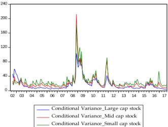
Figure 1 shows the dynamics of real returns and conditional volatility for the three U.S. stock caps (Large, Mid and Small) and WTI oil price. While stock returns are computed as previously defined, the conditional volatility is generated as the GARCH variance from the AR(1) speci-fication of the respective stock caps and oil price (see Arouri et al. 2011a; Salisu and Oloko, 2015b). A formal test for volatility by Engle (1982) - (ARCH) test, was conducted and pre-sented in Table 1. The table, in addition to the ARCH test result, presents the descriptive statis-tics and results for Autocorrelation and Normality tests.
Figure 1. Dynamics of real U.S. stock and Oil price returns and volatility.
-30 -20 -10 0 10 20
02 03 04 05 06 07 08 09 10 11 12 13 14 15 16 17
Real return_Large cap stock Real return_mid cap stock Real return_small cap stock
(A): Large cap, Mid cap and Small cap real stock returns
0 40 80 120 160 200 240
02 03 04 05 06 07 08 09 10 11 12 13 14 15 16 17
Conditional Variance_Large cap stock Conditional Variance_Mid cap stock Conditional Variance_Small cap stock
(B): Conditional volatility Large cap, Mid cap and Small cap returns
-40 -30 -20 -10 0 10 20 30
02 03 04 05 06 07 08 09 10 11 12 13 14 15 16 17
Real returns_WTI oil price (C): Real returns_WTI oil price
0 50 100 150 200 250 300 350 400 450
02 03 04 05 06 07 08 09 10 11 12 13 14 15 16 17
Conditional Volatility_Real WTI return (D): Conditional Volatility_Real WTI return
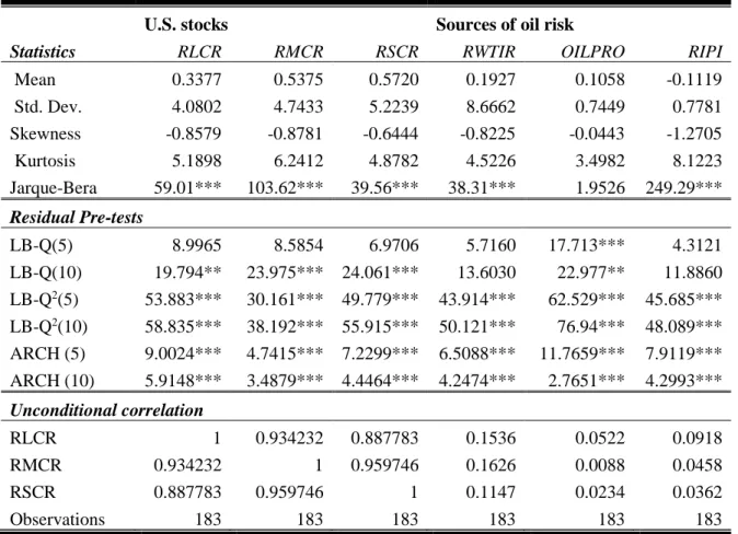
Furthermore, the skewness statistics show that the three categories of U.S. stocks are nega-tively skewed, while the kurtosis statistics show that they are fat tailed. These statistical behav-iours are summarized by Jacque-Bera statistics which conclude that the extent of the skewness and kurtosis of these series are large enough to warrant rejection of normality hypothesis. In addition, evidence from the residual pre-tests as presented in Table 1 suggests that the three stock caps and the three sources of oil price shocks suffer significantly from higher order auto-correlation and conditional heteroscedasticity. To remedy these statistical problems and account for relevant exogenous variables such as proxies for the sources of real oil demand and supply shocks, the relevance of VARMAX-DCC-GARCH is further justified.
Also, the result for the common break in multivariable model conducted using Bai et al. (1998) suggests that there is a significant common structural break between real WTI oil price and the three categories of U.S. stocks3 (see Table 2). In addition, with the pairwise
unconditional correlation of the three U.S. stock caps with real WTI oil price having relatively higher correlation compared with that of U.S. industrial production and global oil production, it suggests that WTI oil price may have higher direct impact on U.S. stock than other sources of oil shock. Hence, aside being identified as the direct source of oil shock by Kilian (2009), this further reinforces the direct impact of WTI oil price in our model specification.
3 Bai et al. (1998) asymptotically determine valid confidence intervals for the date of a single break in multivariate time series,
Table 1. Descriptive statistics.
Statistics
U.S. stocks Sources of oil risk
RLCR RMCR RSCR RWTIR OILPRO RIPI
Mean 0.3377 0.5375 0.5720 0.1927 0.1058 -0.1119
Std. Dev. 4.0802 4.7433 5.2239 8.6662 0.7449 0.7781
Skewness -0.8579 -0.8781 -0.6444 -0.8225 -0.0443 -1.2705
Kurtosis 5.1898 6.2412 4.8782 4.5226 3.4982 8.1223 Jarque-Bera 59.01*** 103.62*** 39.56*** 38.31*** 1.9526 249.29***
Residual Pre-tests
LB-Q(5) 8.9965 8.5854 6.9706 5.7160 17.713*** 4.3121
LB-Q(10) 19.794** 23.975*** 24.061*** 13.6030 22.977** 11.8860 LB-Q2(5) 53.883*** 30.161*** 49.779*** 43.914*** 62.529*** 45.685***
LB-Q2(10) 58.835*** 38.192*** 55.915*** 50.121*** 76.94*** 48.089***
ARCH (5) 9.0024*** 4.7415*** 7.2299*** 6.5088*** 11.7659*** 7.9119***
ARCH (10) 5.9148*** 3.4879*** 4.4464*** 4.2474*** 2.7651*** 4.2993***
Unconditional correlation
RLCR 1 0.934232 0.887783 0.1536 0.0522 0.0918
RMCR 0.934232 1 0.959746 0.1626 0.0088 0.0458
RSCR 0.887783 0.959746 1 0.1147 0.0234 0.0362
Observations 183 183 183 183 183 183
Source: Computed by the authors.Note: RLCR – Real Large Cap Returns; RMCR – Real Mid Cap Returns; RSCR – Real Small Cap Returns; RWTIR – Real Oil Price (WTI) Returns; OILPRO – Crude Oil Production (Percentage change); RIPI –Rate of Change in Demand (using Industrial Production Index as a proxy). Asterisks ***,** and * indicate rejection of null at 1%, 5% and 10% respectively. Ljung-Box Q-statistic test for autocorrelation is evaluated by LB-Q and LB-Q2statistics, while F-statistics for the
ARCH test by Engle (1982) are also presented. The significance of the statistics implies the rejection of null hypothesis of no serial correlation and no Autoregressive Conditional Heteroscedasticity (ARCH) for Ljung-Box Q-statistic and ARCH tests, re-spectively.
Table 2. Results for Common structural break test.
Variables Optimal lag Sample k ˆ 90% Conf. Int. Sup-W-15%
RLCR, RWTIR 1 2002:06-2017:09 2009:03 2005:01-2013:05 1.4953 (0.00) RMCR, RWTIR 1 2002:06-2017:09 2009:03 2002:11-2016:03 0.9688 (0.00) RSCR, RWTIR 1 2002:06-2017:09 2009:03 2002:11-2016:03 0.9985 (0.00)
Source: Compiled by the authors. Note: kˆ is the common break date determined using Bai et al. (1998) common breaks test. The figures in parenthesis are the p-values computed using the asymptotic distributions of the Sup-W test statistic. The asymptotic and estimation procedure for Sup-W test statistic process is detailed in Bai et al (1998). The optimal lag length is determined using Bayesian Information Criterion (BIC).
4. Empirical results
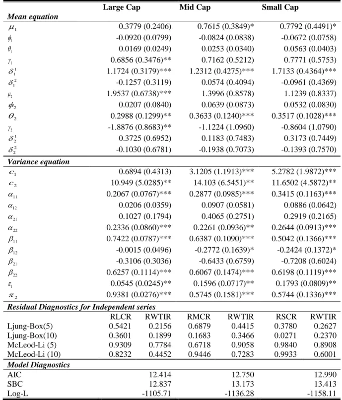
Table 3. Estimation results for VARMAX-DCC-GARCH model.
Large Cap Mid Cap Small Cap
Mean equation
1
0.3779 (0.2406) 0.7615 (0.3849)* 0.7792 (0.4491)*
1
-0.0920 (0.0799) -0.0824 (0.0838) -0.0672 (0.0758)
1
0.0169 (0.0249) 0.0253 (0.0340) 0.0563 (0.0403)
1
0.6856 (0.3476)** 0.7162 (0.5212) 0.7771 (0.5753)
1 1
1.1724 (0.3179)*** 1.2312 (0.4275)*** 1.7133 (0.4364)***
2 1
-0.1257 (0.3119) 0.0574 (0.4094) -0.0961 (0.4369)
2
1.9537 (0.6738)*** 1.3996 (0.8578) 1.1239 (0.8337)
2
0.0207 (0.0840) 0.0639 (0.0873) 0.0532 (0.0830)
2
0.2988 (0.1299)** 0.3633 (0.1240)*** 0.3517 (0.1028)***
2
-1.8876 (0.8683)** -1.1224 (1.0960) -0.8604 (1.0790)
1 2
0.3725 (0.6952) 0.1183 (0.7483) 0.3173 (0.7449)
2 2
-0.1030 (0.6781) -0.1938 (0.7073) -0.1393 (0.7570) Variance equation
1
c 0.6894 (0.4313) 3.1205 (1.1913)*** 5.2782 (1.9872)***
2
c 10.949 (5.0285)** 14.103 (6.5451)** 11.6502 (4.5872)**
11
0.2067 (0.0767)*** 0.2877 (0.0985)*** 0.3415 (0.1163)***
12
0.0206 (0.0359) 0.0907 (0.0581) 0.0886 (0.0642)
21
0.1027 (0.1794) 0.4065 (0.2751) 0.2919 (0.2165)
22
0.2336 (0.0860)*** 0.2261 (0.0936)** 0.2644 (0.0913)***
11
0.7422 (0.0787)*** 0.6387 (0.1090)*** 0.5042 (0.1366)***
12
-0.0015 (0.0496) -0.2772 (0.1639)* -0.2424 (0.1372)*
21
-0.3106 (0.3036) -0.6433 (0.6759) -0.7208 (0.6024)
22
0.6257 (0.1114)*** 0.6067 (0.1474)*** 0.6198 (0.1119)***
1
0.0545 (0.0245)** 0.1596 (0.0717)** 0.1793 (0.0809)**
2
0.9381 (0.0276)*** 0.5745 (0.1581)*** 0.5744 (0.1336)*** Residual Diagnostics for Independent series
RLCR RWTIR RMCR RWTIR RSCR RWTIR Ljung-Box(5) 0.5421 0.2156 0.6879 0.4415 0.3780 0.2627 Ljung-Box(10) 0.3601 0.1899 0.1683 0.3466 0.0271 0.2370 McLeod-Li (5) 0.9309 0.7784 0.6718 0.9058 0.9840 0.8908 McLeod-Li (10) 0.8232 0.4452 0.9446 0.7283 0.9933 0.6001 Model Diagnostics
AIC 12.414 12.750 12.990
SBC 12.837 13.173 13.413
Log-L -1105.71 -1136.28 -1158.11
Note: Asterisks ***, ** and * indicate significance at 1%, 5% and 10% levels respectively. The parameters are as described in the model. Meanwhile, subscript “1” indicates real stock caps while subscript “2” indicates real oil price. In the variance equation model, subscript “11” and “22” indicate own shocks or volatility spillovers while subscript “12” and “21” represent cross-market shocks or volatility spillovers. Superscript “1” and “2” in the mean equation indicate real economic activity demand and global oil production respectively. Also, figures in parenthesis and residual diagnostics are presented in probability values.
of the market segment being considered. But, considering the effect of oil price volatility/risk
on U.S. stock market volatility as indicated by the coefficient of (12), it may be observed that the volatility spillover from oil to the mid cap and small cap stocks is statistically significant, but not statistically significant for large cap stocks. This implies that higher volatility in oil market induces higher volatility in the mid cap and small cap segments of the U.S. stock market but not in the large cap segment. This may result from the fact that investors in large cap stock market are panic less in the face of high oil price risk/volatility, as the market is highly interna-tionalized and liquid (see Oloko, 2017). The relatively insignificant responsiveness of large cap stock market to oil price risk as against the mid cap and small cap stock markets confirms our position in this study. Apparently, it confirms that making generalization about U.S. stock mar-ket’s reaction to oil price risk/volatility without making specific reference to a particular stock market segment being considered may be misleading. This is because large cap reacts to oil price volatility differently from mid cap and small cap.
5. Concluding remarks
This study queries the act of making generalization about the dynamics of returns and volatility spillovers between oil price and U.S. stocks by merely considering only large cap stocks. It argues that this kind of generalization may be misleading, as the reactions of large cap, mid cap and small cap stocks to change in oil prices are not expected to be uniform. Our findings show that the generalization is incorrect when considering the effect of oil risk/volatility on U.S. stock volatility. This is evident as the result shows that the volatility spillover from oil price to the mid cap and small cap stock is statistically significant, but not statistically significant for large cap stock market.
Acknowledgements
The authors wish to thank the two anonymous reviewers and the editor for their useful contribution to the quality of the paper. The first and the third authors acknowledge financial support from the Centre for Econometric & Allied Research (CEAR), University of Ibadan, Nigeria.
References
Alsalman, Z. (2016) Oil price uncertainty and the U.S. stock market analysis based on a GARCH-in-mean VAR model, Energy Economics, 59, 251-260.
Arouri, M., Jouin, J. and Nguyen, D. (2011a) Oil prices and sector stock returns: Implication for portfolio management, International Journal of Money and Finance, 30, 1387-1405. Arouri, M., Lahiani, A., and Nguyen, D. (2011b) Return and volatility transmission between world oil prices and stock markets of the GCC countries, Economic Modelling, 28, 1815–1825.
Bai, J. and Perron, P. (1998) Estimating and Testing Linear Models with Multiple Structural Changes, Econometrica, 66(1), 47-78.
Bai, J., Lumsdaine, R. L. and Stock, J. H. (1998) Testing for Dating Common Breaks in Multivariate Time Series, Review of Economic Studies, 65, 395-432.
Banz, R. W. (1981) The Relationship between Return and Market Value of Common Stocks, Journal of Financial Economics, 9(1), 3-18.
Dias, A. (2013) Market capitalization and Value-at-Risk, Journal of Banking & Finance, 37(12), 5248-5260.
Filis, G., Degiannakis, S. and Floros, C. (2011) Dynamic correlation between stock market and
oil prices: the case of oil-importing and oil-exporting countries, International Review of Financial Analysis 20, 152–164.
Kilian, L. (2009) Not All Oil Price Shocks Are Alike: Disentangling Demand and Supply Shocks in the Crude Oil Market, American Economic Review, 99(3), 1053-1069. Kilian, L. and Park, C. (2009) The Impact of Oil Price Shocks on the US Stock Market,
Inter-national Economic Review 50(4), 1267–1287.
Ling, S. and McAleer, M. (2003) Asymptotic theory for a vector ARMA – GARCH model, Econometric Theory 19, 280– 310.
McAleer, M., Hoti, S. and Chan, F. (2009) Structure and asymptotic theory for multivariate asymmetric conditional volatility, Econometric Reviews 28, 422-440.
Mollick, A.V. and Assefa, T.A. (2013) US stock returns and oil prices: The tale from daily data and the 2008 – 2009 financial crisis, Energy Economics 36, 1 –18.
Oloko, T.F. (2017) Portfolio diversification between developed and developing stock markets: The case study of US and UK investors in Nigeria, Research in International Business and Finance, in press, doi.org/10.1016/j.ribaf.2017.07.153.
Pendse, G. and Slen, E. (2016) A smarter way to approach small cap investing, Nasdaq Global Indexes, 1-7.
Perron, P. (1989) The great crash, the oil price shock and the unit root hypothesis, Econometrica 57, 1361–401.
Quinn, J. (2004) U.S. Stock Indexes: Is there a best choice? Research Report, 1-24.
Sadorsky, P. (1999) Oil price shocks and stock market activity, Energy Economics 21, 449– 469.
Salisu, A. A. and Mobolaji, H. (2013) Modeling returns and volatility transmission between oil price and US–Nigeria exchange rate, Energy Economics, 39, 169-176.
Salisu A.A. and Oloko, T.F. (2015a) Modelling oil price-US stock nexus: A VARMA-BEKK-AGARCH approach, Energy Economics 50, 1-12.
Salisu, A.A. and Oloko, T.F. (2015b) Modelling spillovers between stock market and FX mar-ket: evidence for Nigeria, Journal of African Business 16 (1–2), 84–108.
Salisu, A.A., Isah, K. and Ademuyiwa, I. (2017) Testing for asymmetries in the predictive model of oil-inflation, Economics Bulletin 37 (03), 1797-1804.
Switzer, L. N. (2010) The behaviour of small cap vs. large cap stocks in recessions and recoveries: Empirical evidence for the United States and Canada, North American Journal of Economics and Finance 21, 332-346.