Arne Hillebrand, Han Hoogeveen, Roland Geraerts
Department of Information and Computing Sciences, Utrecht University Princetonplein 5, 3584CC, Utrecht, the Netherlands
[email protected]; [email protected]; [email protected]
Abstract - The quantification of pedestrian safety is an important research topic. If reliable quantification is
possible, it can be used to predict and prevent dangerous situations, such as the crowd crush at the 2010 Love
Parade. To quantify safety, we can use several metrics like density, velocity, flow and pressure. Unfortunately, there are several methods to evaluate these metrics, which may give different results. This can lead to different interpretations of similar situations. Researchers compare these metrics visually or search for trends in fundamental diagrams. This is inherently subjective. We propose an objective methodology to compare these methods, where we emphasize the different quantifications of peak “dangerousness”. Furthermore, we refine existing methods to include the obstacles in environments by replacing the Euclidean distance with the geodesic distance. In our experimental analysis, we observe large differences between different methods for the same scenarios. We conclude that switching to a different method of analysing crowd safety can lead to different conclusions, which asks for standardisation in this research field. Since we are concerned with human safety, we prefer to err on the side of caution. Therefore, we advocate the use of our refined Gaussian-based method, which consistently reports higher levels of danger.
Keywords: pedestrian safety, metrics, analysis, density, velocity, flow, pressure
1. Introduction
At the 2010 Love Parade [6], 21 people were crushed to death and hundreds got injured. In 2006 and 2015 hundreds of pilgrims got trampled during the Hajj to Mecca due to dangerously overcrowded situations [7]. Motivated by such disasters, researchers study ways of preventing these from happening again. By studying metrics like density, velocity, flow and pressure, early warning signs for potentially dangerous situations can be found.
In this paper, we refer to density, velocity, flow and pressure as metrics. Different methods exist to evaluate them. For density, the best-known method is the grid-based method [5]. A regular grid is superimposed on the environment, dividing the environment into cells. Another way of determining density uses Gaussian distributions [7,12]. Such methods place two-dimensional Gaussian distributions on the pedestrian’s locations. By adding the Gaussian distributions together, a density field is formed. A third method to determine local density uses Voronoi diagrams [13]. A Voronoi diagram is a division of the environment in cells, such that all points within a cell are closest to a single pedestrian. The density within each cell is 1 divided by the area of the cell. Details for these methods can be found in Section 2.1.
It is possible to determine the velocity by using density [15]. Using the density and velocity, both flow and pressure can be determined [7]. We describe their implementation in Section 2.2.
Fruin [5] computes the danger level based on the value of these metrics within a (small) region of the environment, which is mapped to six non-overlapping intervals. This method is called Level of Service (LoS). The different intervals encode situations from safe to dangerous. The exact boundaries of these intervals depend on different factors, such as the measurement location and even culture [1].
Duives et al. [4] compare density methods using fundamental diagrams. For different scenarios they formulate what trends they expect to be present in these diagrams, and look for them. One drawback of this method is that it requires expert knowledge about what trends are to be expected. Furthermore, it is inherently subjective due to the human classification step.
Duives et al. [4] also propose an objective measure of similarity between density methods called
scatter. The scatter is the range of measured velocities for non-overlapping density intervals. One downside of this measure is the interdependency between these metrics. A small change in the density method can result in a large shift in the measured scatter due to the potential recategorization of measured velocities.
1.1. Our Contribution
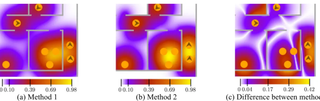
In this paper, we propose an objective methodology for comparing methods that compute safety metrics. We also refine existing methods to consider obstacles in the environment. We achieve this by replacing the Euclidean distance by the geodesic distance [10]. The resulting differences are showcased in Fig. 1. Method 1 uses the Euclidean distance, whereas method 2 uses the geodesic distance.
We also performed experiments on environments to test if our methodology yielded new insights into the differences between methods. We conclude that the classification of a situation as being safe depends on the method that is used, and that our refined methods consistently classify situations as more dangerous.
1.2. Overview
In Section 2, we discuss the different methods used for evaluating the metrics. Here we also introduce our refinements of two methods. Next, in Section 3 we give details of the four measures used to quantify the differences between the methods. These measures are used in Sections 4 and 5 to evaluate the different methods on three basic environments and several scenarios. We end with a conclusion in Section 6.
2. Methods for Measuring Safety
As discussed in Section 1, different metrics exist. Furthermore, there are different methods for computing each metric. In Section 2.1, we discuss different density methods. The considered methods are either grid-, Voronoi- or Gaussian-based. How the resulting density fields can be used to determine velocity, flow and pressure fields will be discussed in Section 2.2.
2.1. Density methods
The grid-based method was first defined by Fruin [5]. Intuitively, this method counts the number of pedestrians in a cell 𝐶𝐶𝑖𝑖, where the cells are defined by a regular grid which is placed over the environment. This grid does not consider the obstacles in the environment. Next, this number is divided by the area 𝐴𝐴𝑖𝑖 of the cell to get the local density. All the pedestrians are considered to be
(a) Method 1 (b) Method 2 (c) Difference between methods
Fig. 1: An environment with pedestrians, represented by orange discs. The environment measures 6𝑚𝑚× 7𝑚𝑚.
discs and measuring the fraction of the disc in a cell.
Steffen and Seyfried [13] take another approach at minimizing these large jumps in density. Their
Voronoi-based method describes the free space that is available to a pedestrian by using Voronoi diagrams. A Voronoi diagram of 𝑛𝑛 input points is the partitioning of the environment into 𝑛𝑛 cells, such that every position within that cell is closest to exactly one point. Steffen and Seyfried [13] use the locations of the pedestrians for calculating a Voronoi diagram as the input points. After obtaining this diagram, the density within each Voronoi cell 𝑖𝑖 is defined as 1/𝐴𝐴𝑖𝑖. Here, 𝐴𝐴𝑖𝑖 is the area of
Voronoi cell 𝑖𝑖. Next, this Voronoi cell density is used to calculate the density within grid cells by usinga weighted average of all the Voronoi cells that intersect that grid cell.
One drawback of this method is that the area of a Voronoi cell can be large, while it is locally very dense (e.g. pedestrians on the perimeter of a dense group). To this end, Steffen and Seyfried suggest a limit of 2 square meters on the area of a Voronoi cell. Furthermore, it is not mentioned how the obstacles should be handled. In our experiments with the Voronoi method, we will remove the area of a cell that is covered by obstacles. As a result, higher (more accurate) densities are reported.
However, only removing obstructed regions from a Voronoi cell can still give the illusion of too much free space. We show an example of this in Fig. 2(b). Here, a Voronoi cell is split into two disconnected pieces by an obstacle. To remedy this, we propose to use a geodesic Voronoi diagram [10], which accounts for the obstacles in an environment. This also changes the shape of the Voronoi cells. We exemplify this in Fig. 2(b) and (c). Some line segments are replaced by curves, because of the nearby obstacles.
Gaussian-based methods measure density for points instead of areas. Here, the contribution of a pedestrian to a point depends on the distance between the pedestrian and the point. This distance is used as input for a function 𝑓𝑓 that determines the contribution. More formally, the density at point 𝑙𝑙
is defined as 𝜌𝜌(𝑙𝑙) =∑𝑝𝑝∈𝑃𝑃𝑓𝑓(𝑒𝑒𝑒𝑒(𝑙𝑙,𝑝𝑝)). Here, 𝑃𝑃 is the set of all pedestrians and 𝑒𝑒𝑒𝑒(𝑙𝑙,𝑝𝑝) is the Euclidean distance between point 𝑙𝑙 and pedestrian 𝑝𝑝.
One of the first methods that uses this is due to Helbing et al. [7]. They use the following function:
𝑓𝑓(𝑥𝑥) =𝜋𝜋𝑅𝑅12
𝑒𝑒
−𝑥𝑥𝑅𝑅22 (1)This equation is a variation of a Gaussian distribution. Here, 𝑥𝑥 is the distance between a pedestrian and a point. 𝑅𝑅 is the only parameter of this method. It influences the pedestrian’s contribution to the perceived density. Duives et al. [4] point out that 𝑅𝑅 influences the contribution and should be picked carefully.
Plaue et al. [12] suggest a method that bypasses this issue altogether. Instead of having 𝑅𝑅 as a fixed parameter, it is dependent on the current locations of the pedestrians at time 𝑡𝑡. With all locations given as 𝑃𝑃(𝑡𝑡), the function used to determine 𝑅𝑅 for a pedestrian at location 𝑝𝑝 is
𝑒𝑒𝑞𝑞(𝑝𝑝) =� � 𝑒𝑒𝑒𝑒(𝑝𝑝,𝑝𝑝′)−𝑞𝑞 𝑝𝑝′∈𝑃𝑃(𝑡𝑡), 𝑝𝑝≠𝑝𝑝′
� −1𝑞𝑞
(2)
In their experiments the parameter 𝑞𝑞 is set to 4.
resulting in higher local densities. This becomes clear when we compare Figs. 2(d) and 2(e). However, this method still increases the density at the opposite side of an obstacle. In our example, we can see that there is a region with higher density close to walls because of the presence of pedestrians at both sides.
To further take the obstacles into account, we use the geodesic distance. When two pedestrians have the same Euclidean distance to a measurement point, they should not always contribute equally to the local density, because one or more obstacles may cause a detour for the pedestrian. The geodesic distance takes this detour into account. Such a geodesic Gaussian density field can be seen in Fig. 2(f).
2.2. Derived Metrics
Although density is an important metric for determining pedestrian safety, it is not the only one available. We mentioned velocity, flow and pressure in Section 1 and gave an intuitive definition. In this section, we will show how these metrics can be determined.
To compute (local) velocities, we use an adaptation of the method described in Helbing et al. [7, Equation 6]. In this method, the local velocity is defined as:
𝑉𝑉�⃗(𝑙𝑙,𝑡𝑡) = ∑∑𝑝𝑝∈𝑃𝑃(𝑡𝑡)𝑣𝑣⃗𝑝𝑝𝑓𝑓𝑓𝑓(𝑙𝑙(,𝑙𝑙𝑝𝑝,𝑝𝑝))
𝑝𝑝∈𝑃𝑃(𝑡𝑡) (3)
Here, 𝑙𝑙 is a location, 𝑡𝑡 is the current time, 𝑃𝑃(𝑡𝑡) is the set of locations of the pedestrians, 𝑣𝑣⃗𝑝𝑝 is the
velocity of the pedestrian at location 𝑝𝑝 and 𝑓𝑓(𝑙𝑙,𝑝𝑝) is a weighing factor. Helbing et al. use a Gaussian distance-dependent function for the weighing factor. This is the same function as given in Eq. 1.
Since we used different density methods, we will have 𝑓𝑓(𝑙𝑙,𝑝𝑝) reflect this. That is, we use different definitions of 𝑓𝑓(𝑙𝑙,𝑝𝑝) for the grid-, Voronoi- and Gaussian-based methods respectively. We do this to better reflect the underlying division of the environment in regions. These functions are given in Eqs. 4 through 6. In these equations, 𝑝𝑝 is the location of a pedestrian, 𝐶𝐶𝑖𝑖 is a cell used by
the density method, 𝑙𝑙 a point and 𝐴𝐴𝑝𝑝 is the area for the Voronoi cell 𝑉𝑉𝑝𝑝. Finally, the function 𝑒𝑒(𝑙𝑙,𝑝𝑝) is the geodesic distance gd(𝑙𝑙,𝑝𝑝) when evaluating our refined method, and the Euclidean distance 𝑒𝑒𝑒𝑒(𝑙𝑙,𝑝𝑝) in the other situations.
𝑓𝑓𝐺𝐺𝐺𝐺𝑖𝑖𝐺𝐺(𝐶𝐶𝑖𝑖,𝑝𝑝) =� 0,1, 𝑜𝑜𝑡𝑡ℎ𝑒𝑒𝑒𝑒𝑤𝑤𝑖𝑖𝑒𝑒𝑒𝑒𝑖𝑖𝑓𝑓𝑝𝑝 ∈ 𝐶𝐶𝑖𝑖 (4)
𝑓𝑓𝑉𝑉𝑉𝑉𝐺𝐺𝑉𝑉𝑉𝑉𝑉𝑉𝑖𝑖(𝑙𝑙,𝑝𝑝) =�
1
𝐴𝐴𝑝𝑝, 𝑖𝑖𝑓𝑓𝑙𝑙 ∈ 𝑉𝑉𝑝𝑝
0, 𝑜𝑜𝑡𝑡ℎ𝑒𝑒𝑒𝑒𝑤𝑤𝑖𝑖𝑒𝑒𝑒𝑒
(5)
𝑓𝑓𝐺𝐺𝐺𝐺𝐺𝐺𝐺𝐺𝐺𝐺𝑖𝑖𝐺𝐺𝑉𝑉(𝑙𝑙,𝑝𝑝) =𝜋𝜋𝑅𝑅12
𝑒𝑒
−𝑒𝑒(𝑙𝑙,𝑝𝑝)
𝑅𝑅2 (6)
(a) Classical [5] (b) Voronoi [13] (c) Voronoi (geo) (d) Gaussian [7] (e) Gaussian [12] (f) Gaussian (geo) Fig. 2: Different density fields. The orange disks represent pedestrians. (a): Fruin's classical density [5] with
𝑤𝑤= 1𝑚𝑚. (b) and (c): The Voronoi diagram as used by Steffen and Seyfried [13] and the geodesic Voronoi
diagram. (d), (e) and (f): The Gaussian-based density method by Helbing et al. [7] with 𝑅𝑅 = 1𝑚𝑚, the method
𝑙𝑙,𝑡𝑡 𝐶𝐶 𝐶𝐶 𝐶𝐶 𝑋𝑋 of the points in region 𝐶𝐶.
3. Comparing different methods
From Fig. 2 it is clear that different methods can give different results, but are these differences significant? We will look at four measures for comparing these methods to try and answer that question.
When we analyse a method 𝑀𝑀, we will look at a region of interest 𝑅𝑅 within the studied environment. This area is divided into a set of cells 𝐶𝐶𝑖𝑖 for 1≤ 𝑖𝑖 ≤ 𝑁𝑁. These cells follow from the
method we choose. The value for such a cell is given by 𝑣𝑣(𝐶𝐶𝑖𝑖,𝑀𝑀).
First, we look at the maximal value for 𝑀𝑀 within 𝑅𝑅, which enables us to compare measured peak densities, velocities, flows and pressures. We also look at the maximal difference between two methods. They are given in Eqs. (7) and (8).
max
(𝑀𝑀) = 1≤𝑖𝑖≤𝑁𝑁max
𝑣𝑣(𝐶𝐶𝑖𝑖,𝑀𝑀) (7)max
(𝑀𝑀1,𝑀𝑀2) = 1≤𝑖𝑖≤𝑁𝑁max
|𝑣𝑣(𝐶𝐶𝑖𝑖,𝑀𝑀1)− 𝑣𝑣(𝐶𝐶𝑖𝑖,𝑀𝑀2)| (8)These two measures do not offer more information than a visual inspection. The differences are accented, but other information is lost. For that reason, we introduce two new measures. For these measures it is important that 𝑅𝑅 is centred within the area we want to study. This, however, should not be a problem since we are interested in local values. We call the first one the quadratic score (qs). We define it as follows:
𝑞𝑞𝑒𝑒(𝑀𝑀) = 𝐴𝐴1
𝑅𝑅� �
𝑣𝑣(𝐶𝐶𝑖𝑖,𝑀𝑀)
max
(𝑀𝑀)�𝑁𝑁
𝑖𝑖=1
2
𝐴𝐴𝑖𝑖 (9)
Here, 𝐴𝐴𝑖𝑖 is the obstacle-free area of cell 𝐶𝐶𝑖𝑖 and 𝐴𝐴𝑅𝑅 =∑𝑁𝑁𝑖𝑖=1𝐴𝐴𝑖𝑖 is the obstacle-free area of 𝑅𝑅.
The resulting value is a number in the range of 0 to 1. A value of 1 denotes that all 𝑁𝑁 cells are at the maximal value. When 𝑞𝑞𝑒𝑒 gets closer to 0, it means that a large area of 𝑅𝑅 has low values. This function ensures that regions which are closer to high (i.e. dangerous) values are emphasized. Furthermore, this method evaluates to simple scalars. Therefore, it is possible to use existing statistical methods to determine if there is a statistically significant difference.
The last measure we discuss is a comparison based on how the industry often interprets the values from the metrics. Usually, a certain threshold value is used or categories are specified. An example is the LoS concept [5]. Eq. 10 calculates the difference in categorization between two different methods.
𝑏𝑏𝑒𝑒(𝑀𝑀1,𝑀𝑀2) = 𝐴𝐴𝑅𝑅1 � �𝑏𝑏𝑖𝑖𝑛𝑛(𝐶𝐶𝑖𝑖,𝑀𝑀1)− 𝑏𝑏𝑖𝑖𝑛𝑛(𝐶𝐶𝑖𝑖,𝑀𝑀2)�2 𝑁𝑁
𝑖𝑖=1 𝐴𝐴𝑖𝑖 (10)
Here, 𝑏𝑏𝑖𝑖𝑛𝑛(𝐶𝐶𝑖𝑖,𝑀𝑀) is a function that maps 𝑣𝑣(𝐶𝐶𝑖𝑖,𝑀𝑀) to the category's number. For example, when a
single threshold 𝑡𝑡 is given, a value 𝑣𝑣(𝐶𝐶𝑖𝑖 ,𝑀𝑀) < 𝑡𝑡 maps to 0 and all other values to 1. A higher
score means that there are many differently classified cells. The difference between the classifications is squared to emphasize larger differences.
4. Experimental Setup
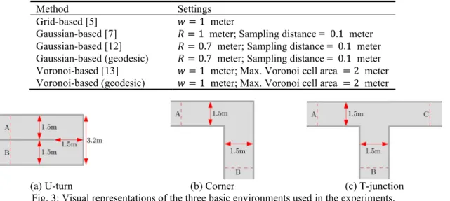
methods are shown in Table 1. The Voronoi-based method is the one that Steffen and Seyfried [13] refer to as 𝐷𝐷𝑉𝑉.
We tested the methods on the three environments depicted in Fig. 3. These environments are building blocks for larger environments and are frequently used in studies [2,3]. For both the U-turn and corner environment, simulated pedestrians (agents) moved from line 𝐴𝐴 to line 𝐵𝐵. For the T-junction environment, we tested two different variations. One with one entrance at line 𝐴𝐴 and two exits located at 𝐵𝐵 and 𝐶𝐶 (scenario 1), and one variation where the agents entered from 𝐵𝐵 and 𝐶𝐶
and moved towards 𝐴𝐴 (scenario 2). The agents were created at a random position behind the starting lines. The rate at which the agents were added was varied from 0.5/𝑒𝑒 to 2.5/𝑒𝑒. The agents' preferred speed was set at 1.4 𝑚𝑚/𝑒𝑒.
We recorded the location and velocity of the pedestrians every tenth of a second for 10 simulated minutes, starting 2 minutes after the first pedestrian reached the exit. We used this data to calculate the different fields. We also calculated the time-average fields over a timespan of 1s, 10s and 60s.
5. Results
The analysis of the results is split into three parts. First, we look at how the size of the averaging window influences our analyses. Second, we will perform an in-depth analysis for the U-turn environment to show what information can be extracted using the discussed measures. Third and last, we make general observations for all the different environments tested. We only discuss the 𝑞𝑞𝑒𝑒
and 𝑏𝑏𝑒𝑒 measures. Other results are available on the author’s website [9].
5.1. The Size of the Averaging Window
We analysed the effect of different averaging windows. The size of the averaging windows seems to be of little effect for the Gaussian-based methods when looking at the maximum values. Furthermore, the shape of the curves for the reported maxima stay the same. In case of the quadratic score, some details disappear when we increase the size of the averaging window. We found that averaging windows larger than 10s are not needed. Therefore, we will report all results for an averaging window of 10𝑒𝑒.
5.2. In-depth Analysis of the U-turn Environment
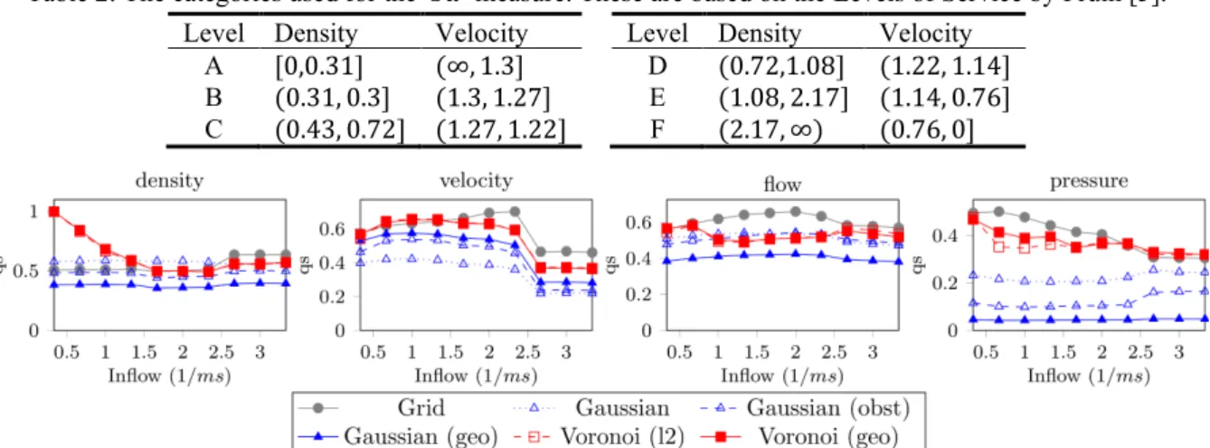
We summarized the results in Figs. 4 and 5. At first glance, it seems that the results for 𝑞𝑞𝑒𝑒 for the Voronoi-based density methods give unexpected results for lower inflows: the entire environment is at the peak density. When the inflow is increased, it steadily declines. This is an artefact of how the Voronoi-based method is defined. Steffen and Seyfried [13] defined a minimal density within all Voronoi cells. When the cells are large enough, the reported local density value is only determined by this maximal area. When the inflow is increased, this setting becomes less and less influential on the maximal measured values.
(a) U-turn (b) Corner (c) T-junction
Fig. 3: Visual representations of the three basic environments used in the experiments. Table 1: Overview of the settings for determining the fields used in the experiments.
Method Settings
Grid-based [5] 𝑤𝑤= 1 meter
Gaussian-based [7] 𝑅𝑅= 1 meter; Sampling distance = 0.1 meter
Gaussian-based [12] 𝑅𝑅= 0.7 meter; Sampling distance = 0.1 meter
Gaussian-based (geodesic) 𝑅𝑅= 0.7 meter; Sampling distance = 0.1 meter
Voronoi-based [13] 𝑤𝑤= 1 meter; Max. Voronoi cell area = 2 meter
Another interesting observation is the ordering of the different Gaussian-based methods. For the density, flow and pressure, the 𝑞𝑞𝑒𝑒 score is always lower, but for velocity it is always higher. This is a result of the use of the geodesic distance. The Gaussian-curves are more localized around the locations of the pedestrians in our version. As a result, less of the curves are on the opposite side of the obstacle and opposing velocities do not cancel each other out near the obstacle. This means that the geodesic Gaussian does not influence the area on the opposite side of the walls.
We also determined the 𝑏𝑏𝑒𝑒 for density and velocity measurements. The bins that were used are shown in Table 2. In case of the Gaussian method, it is interesting to note that the differences according to the velocity measurements were much bigger. It is also interesting to see that the Voronoi-based methods also show differences, although the 𝑞𝑞𝑒𝑒 was similar for all different inflows. However, at what inflow these differences register differs greatly on what metric we use. Further research is needed to determine what metric is more suitable or if more metrics should be used in conjunction.
5.3. Analyses of All Environments
For all tests for statistical significance we used ANOVA with a significance level of 0.05. For each environment, we performed statistical analyses for 𝑞𝑞𝑒𝑒 and 𝑏𝑏𝑒𝑒. This reported that there were differences between the different methods. Using Tukey-HSD post-hoc analyses, we found that at almost all flows, all methods were different from each other at almost all levels of inflow.
The situations where these differences were insignificant were at the lower inflows for the Voronoi-based methods. This is probably a result of the maximal Voronoi cell size, as discussed in Section 5.2. For the other environments, similar results were found. That is, the geodesic Gaussian consistently reports higher values than the other Gaussian-based methods. The two Voronoi-based methods seem to generate similar results (although the differences are still significant).
Therefore, we cannot simply use one cut-off point for determining if a situation is safe. This is already widely known when looking at different situations and cultures, but to the best of our knowledge it was not yet shown for different methods. This asks for standardisation in this research field.
Fig. 4: The different 𝑞𝑞𝑒𝑒 valies for the U-turn environment. The averaging window is set to 10 seconds.
Fig. 5: The different 𝑏𝑏𝑒𝑒 values for the U-turn environment. The averaging window is set to 10 seconds. Upper
6. Conclusion
In this paper, we have discussed different metrics for evaluating pedestrian safety. Each metric can be evaluated by several different methods. We described a refinement for existing methods, namely the usage of the geodesic instead of the Euclidean distance, which takes obstacles into account. We have shown experimentally that this change results in significantly higher densities, flows and pressures.
Furthermore, we discussed four measures for comparing different methods. The maximum (𝑚𝑚𝑉𝑉𝑥𝑥) and maximum difference (𝑚𝑚𝑉𝑉𝑥𝑥𝑒𝑒𝑖𝑖𝑓𝑓𝑓𝑓) are already used to show differences between two methods. We introduced the quadratic score (𝑞𝑞𝑒𝑒) and bin distance (𝑏𝑏𝑒𝑒) to better show the differences between methods. We analysed all methods by using these four measures and concluded that the differences between the methods are significant. Since we are concerned with human safety, we prefer to err on the side of caution. Therefore, we advocate the use of our method, which consistently reports higher levels of “danger”.
One major selling point of analysing the differences between different methods using 𝑚𝑚𝑉𝑉𝑥𝑥,
𝑚𝑚𝑉𝑉𝑥𝑥𝑒𝑒𝑖𝑖𝑓𝑓𝑓𝑓, 𝑞𝑞𝑒𝑒 and 𝑏𝑏𝑒𝑒 is that it leaves no room for subjective interpretation of the results. As a result, any researcher performing a similar study should be able to end up with similar conclusions.
6.1. Future Work
Although the measures described in this paper show that there is a difference between different methods, it is still not easy to explain what causes them. Therefore, it stays important to look at renderings of the respective fields. It would be interesting to research if there is an automatic classification possible that captures what causes the differences. Furthermore, we only tested on smaller environments. We still need to determine if these measures are effective for larger environments, such as a building or a city.
It would also be interesting to see how the geodesic distance influences the measurements for the different metrics on multi-layered environments [8]. Previously, this was difficult because the Euclidean distance for pedestrians in multi-layered environments is not well defined, but the geodesic distance is. Therefore, it is possible to use the two methods described in this paper for multi-layered buildings.
References
[1] U. Chattaraj, A. Seyfried and P. Chakroborty, “Comparison of pedestrian fundamental diagram across cultures,” Advances in Complex Systems, vol. 12, no. 3, pp. 393–405, 2009.
[2] M. Creasemeyer and A. Schadschneider, “Simulation of Merging Pedestrian Streams at
T-Junctions: Comparison of Density Definitions,” Traffic and Granular Flow ’13, pp. 291-298, 2015
[3] C. Dias and R. Lovreglio, “Calibrating cellular automaton models for pedestrians walking through corners”, Physics Letters A, vol. 382, no. 19, pp. 1255-1261, 2018
[4] D.C. Duives, W. Daamen, and S.P. Hoogendoorn, “Quantification of the level of crowdedness for pedestrian movements,” Physica A: Statistical Mechanics and its Applications, vol. 427, pp. 162– 180, 2015.
[5] J.J. Fruin, “Pedestrian planning and design,” Technical report, 1971.
[6] D. Helbing and P. Mukerji, “Crowd disasters as systemic failures: analysis of the love parade disaster,” EPJ Data Science, vol. 1, no. 1, 2012.
[7] D. Helbing, A. Johansson, and H. Z. Al-Abideen, “Dynamics of crowd disasters: An empirical study,” Physical review E, vol. 75, no. 4, 2007.
[8] A. Hillebrand, M. van den Akker, R. Geraerts, and H. Hoogeveen, “Performing multicut on walkable environments,” International Conference on Combinatorial Optimization and Applications, Hong Kong, 2016, vol. 10043, pp. 311–325.
[12] M. Plaue, G. Bärwolff and H. Schwandt, “On measuring pedestrian density and flow fields in dense as well as sparse crowds,” Pedestrian and Evacuation Dynamics 2012, Zurich, 2014, vol. 1, pp. 411–424.
[13] B. Steffen and A. Seyfried, “Methods for measuring pedestrian density, flow, speed and direction with minimal scatter,” Physica A: Statistical mechanics and its applications, vol. 389, no. 9, pp. 1902–1910, 2010.
[14] W. van Toll, N. Jaklin, and R. Geraerts, “Towards believable crowds: A generic multi-level framework for agent navigation,” ASCI.OPEN, 2015.