Optimizing a bi-objective vendor-managed inventory of multi-product EPQ model for a green supply chain with stochastic constraints

(1)

1

Optimizing a bi-objective vendor-managed inventory of

multi-product EPQ model for a green supply chain with stochastic

constraints

* 1

, Seyed Hamid Reza Pasandideh

1

Poshtahani

Saeide Jamshidpour

1_{Department of Industrial Engineering, Faculty of Engineering, Kharazmi University,} Tehran, Iran

[email protected], [email protected]

Abstract

In this paper, a bi-objective multi-product single-vendor single-buyer supply chain problem is studied under green vendor-managed inventory (VMI) policy based on the economic production quantity (EPQ) model. To bring the model closer to real-world supply chain, four constraints of model including backordering cost, number of orders, production budget and warehouse space are considered stochastic. In addition to holding, ordering and backordering costs of the VMI chain, the unused storage space cost is also added to the total cost of the chain. To observe environmental requirements and decrease the adverse effects of greenhouse gases emissions (GHGs) on the earth and human’s life, green supply chain is utilized to reduce the GHGs emissions through storage and transportation activities in the second objective function. Three multi-objective decision making methods namely, LP-metric, Goal attainment and multi-choice goal programming with utility function (MCGP-U) are implemented in different sizes to solve the presented model as well. Two multi-criteria decision making (MCDM) approach and statistical analysis are applied to compare the outcomes of three proposed solving methods. GAMS/BARON software is utilized to minimize the values of the objective functions. At the end, numerical examples are presented to represent the application of the mentioned methodology. To come up with more insights, sensitivity analysis is executed on the main parameters of proposed model.

Keywords: Economic production quantity (EPQ), vendor-managed inventory (VMI), greenhouse gases (GHGs) emissions, stochastic programming, bi-objective non-linear model.

1- Introduction

In today's progressively competitive business world, companies are trying to increase customer’s satisfaction by reducing their costs and increasing customer’s service levels. For instance, accommodating supply with demand, decreasing stock-outs, and increasing customer delivery times would be appropriate in this case. In this way, the success of companies is related to the efficient flow of products to customers, and without coordinated decisions between their members, the success of companies would not be achieved (Fugate, Sahin, & Mentzer, 2006). As a result, the supply chain is used to communicate among supply chain members. In today’s global markets, supply chain management (SCM) plays a crucial role to make a long-term cooperative relationship among organizations and companies in order to gain either a tensionless constant source of supply and demand of products, or optimum profit from each other, as well as reliability to achieve better performances and (Simchi-Levi, Kaminsky, Simchi-Levi, & Shankar, 2007).

*Corresponding author

Vol. 13, No. 1, pp. 1-34 Winter (January) 2020

(2)

2

Inventory is one of the important factors in SCM. In a supply chain, unpleasant or fluctuating inventory, leads to Bullwhip effect and Double marginalization and eventually undermines supply chain’s performance and may even contributes to the failure of companies (Disney, & Towill, 2003). Among several strategies of collaboration and coordination between supply chain (SC) partners, vendor-managed inventory (VMI) has been successfully implemented in many companies (Disney, & Towill, 2002). It has been used widely in recent years because of its profits. It accelerates the supply chain, improve the profitability for both vendors and customers, and remove the effects of bullwhip in supply chain management. The benefits of VMI are well recognized by successful retail businesses such as Wal-Mart, JC Penney, and Dillard Department Stores (Dong & Xu, 2002). Successful VMI implementation in retailing are more observable in the apparel industry. For example, VF Corporation was able to increase the sales of its men’s jeans by 20% through the adoption of a replenishment system based on point-of-sales data and VMI principles (Kaipia & Tanskanen, 2013). All of this evidence proves that the potential advantages of the VMI partnerships have a powerful effect and can be mentioned as a significant tool in order to reduce inventory costs for supply chain members and enhance customer service levels (Achabal, McIntyre, Smith, & Kalyanam, 2007).

The gradual increases of global warming and climate change have enforced industries and governments to reduce their greenhouse gases emissions to improve environmental sustainability. Nowadays, several businesses have launched to perform green supply chain management and pay attention to environmental issues and measure their vendors’ environmental performance. Inventory management and transportation are the major activities of supply chain that create the significant amount of greenhouse gases emissions in numerous studies. In reality, inventory control is a crucial activity in many types of organization (Tsou, Hsu, Chen, & Yeh, 2010). The inventory management of a company depends on the frequency of it transportation and storage process, so it is one of the main determinants of the greenhouse gases created in supply chain (Schaefer & Konur, 2015). As a result, current research aims to reduce the greenhouse gases emissions released through transportation and storage activities. In recent studies (Büyüközkan, & Cifci, 2013; Bonney, & Jaber, 2011; Zanoni, Mazzoldi, & Jaber, 2014), merging environmental requirements with inventory and logistics systems has been strongly emphasized. A joint consequence among these models is that the efficiency of an inventory policy becomes sensitive when greenhouse gases (GHGs) emissions are considered. On the other hand, extending the traditional EPQ model by adding effective constraints and objective function, and taking into account the parameters of model in an uncertain way by using stochastic programming approach, bring the EPQ model closer to real-world conditions.

In the next section, First, a brief review of research done on the effects of implementing VMI policy on whole supply chain is represented, and then some research worked on the environmental effects due to greenhouse gases emissions on inventory management are presented.

2- Literature review

Cetinkaya & Lee (2000) proposed a harmonized inventory and transportation analytical model Applicable in VMI systems. In particular, they considered a vendor who satisfied a sequence of retailers' demand in a particular geographic area. Ideally, these demands must be shipped immediately. Dong & Xu (2002) evaluated the effects of VMI on a supply channel. In a nutshell, they showed that VMI is found to reduce total costs of the channel system and it could increase the profitability of both vendor and buyer in the chain system. Yao, Evers, Dresner (2007) developed an analytical model that examines the effects of supply chain's parameters on cost savings. They used common initiatives, such as VMI system. The results of the model showed that the benefits, in the form of reducing inventory costs, might have been created according to the ratio of product integrity to the supplier's ordering costs to the buyer and the proportion of transportation cost to the buyer. The results also illustrated that vendor and buyer have equal share in the amount of benefits. Razmi, Rad, Sangari (2010) provided a two-echelon supply chain, including single buyer-single supplier assuming that the supplier meets only one buyer as the contract party. They compared the performance of the traditional system with VMI system and showed that VMI is a better approach than the traditional model and causes lower cost in all conditions. Pasandideh, Niaki, & Roozbeh Nia (2010) proposed a two-level economic order quantity (EOQ) model for a single supplier-single retailer in a supply chain under VMI policy. An analytical model has been investigated to examine the impact of important supply chain’s parameters on reducing costs in an integrated supply chain under backlogged shortage,

(3)

3

and the results of the analysis have been compared before and after implementation of VMI. Roozbeh Nia, Hemmati Far, & Niaki (2013) introduced fuzzy multi-products, multi-constraints economic order quantity (EOQ), including a single vendor-single buyer under VMI policy with the goal of minimizing total cost of supply chain. Ant colony optimization algorithm were used to find the near optimal solutions. In order to validate the obtained results a genetic algorithm (GA) and a differential evolution were presented. Bakeshlu, Sadeghi, Poorbagheri, & Taghizadeh (2014) presented a bi-objective two-echelon single vendor-single retailer model under VMI Policy with shortage. The first objective function was to minimize the inventory costs, and the second objective function aimed to minimize the warehouse space. Limits on the number of orders and budget were also presented to bring the model closer to reality. Particle Swarm Optimization (PSO) metaheuristic algorithm was implemented to solve the model. Sadeghi & Niaki. (2015) presented a bi-objective vendor-managed inventory model under two-echelon consisting of single vendor-multi retailers in which demand was considered fuzzy by using trapezoidal fuzzy number. The first goal was minimizing inventory costs and the second goal minimized the storage space. In this model, Limits on the number of orders and budget were applied in constraints. Non-dominated sorting genetic algorithm-II (NSGA-II), multi-objective evolutionary algorithm (MOEA), and non-dominated ranking genetic algorithm (NRGA) were implemented to solve the model. Park, Yoo, & Park (2016) proposed an inventory routing problem with lost sales under a vendor-managed inventory strategy in a two-echelon supply chain consisting of a single manufacturer and multiple retailers. They used Genetic algorithm (GA) to determine either replenishment times and quantities, or vehicle routes while maximizing the supply chain profits. Alfares & Attia (2017) proposed integration between quality control and inventory control in supply chain management. They presented vendor-managed inventory (VMI) and a consignment stock (CS) partnership with several buyers, and considered three different levels of supply, including VMI–CS system, traditional system, and integrated system. They also considered the cost of inspection errors. The products produced by the vendor were not perfect and the proportion of them was defective and the quality inspection of these items was done by buyers. Han, Lu, & Zhang (2017) proposed an indirect VMI problem in a three-echelon supply chain in which distributors (third-party logistics companies) took responsibility to balance between a vendor (manufacturer) and multiple buyers (manufacturers). They used vertex enumeration algorithm to solve their three-echelon decision making model. Bonny & Juber (2011) examined the importance of inventory control systems to considerate environmental concerns, and presented that the traditional Economic order quantity (EOQ) model does not have enough efficiency to cover some of the inventory models. Roozbeh Nia, Hemmati Far, & Niaki (2015) presented a multi-product single vendor-single buyer economic order quantity model under backorder and green approach. In their model, they used limited-capacity pallets to transport items. To implement the green approach, they used tax costs for greenhouse gas (GHG) and limitation on GHG emissions. In order to find a near optimal solution, the integrated of genetic and imperialist algorithms was proposed, and they also implemented the genetic algorithm to evaluate the results. Jiang, Li, Qu, & Cheng (2015) proposed a green VMI model with considering both environmental and economic goals. They compared their model with traditional VMI model. The impacts of important factors of carbon emissions and carbon cap were examined analytically on the optimal decisions, the carbon emissions and the total costs of supply chain. Karimi, Niknamfar, Pasandideh (2016) merged a two-level newsboy problem (NP) supply chain model with the supplier selection problem. In order to apply the green approach, the greenhouse gas emissions that are released by the various types of selected vehicles were limited. Alvarado, Paquet, Chaabane, & Amodeo (2016) considered the impacts of environmental regulations on businesses and inventory control systems, and provided demand for both manufacturing and remanufacturing, due to differences in costs and emissions of greenhouse gases. They used the Markov decision to solve the model. Mokhtari & Rezvan. (2017) presented a single supplier multi-buyer multi-product model, under the green supply chain and the VMI model. The shortage was allowed in the form of partial backorder, and the goal was to find the amount of economic production and the maximum level of shortage. The total greenhouse gas emissions have been modeled as a green constraint. To solve the model, a decomposition based analytical approach was proposed. Gharaei et al. (2018) presented an Outer Approximation with Equality Relaxation and Augmented Penalty (OA/ER/AP) in order to solve an integrated multi-product multi-buyer green supply chain under the penalty and VMI-CS policies considering real stochastic constraints. Furthermore, the model distinguished between the financial

(4)

4

and non-financial elements of holding costs in which the first and second, included space investment, and the expenditure allocated to physical storage, movement, and security of the products, respectively. Detcharat Sumrit (2019) developed VMI supply chain in healthcare system using fuzzy multi-criteria decision-making approach (MCDM) to determine the best potential supplier which has been performed in one of prominent public hospitals in Thailand as a case study. Three MCDM framework were presented, included Fuzzy Delphi approach to determine the suitable assessment criteria for VMI supplier selection, Fuzzy Step-wise Weight Assessment Ration Analysis (SWARA) method to select the relative importance weight of assessment criteria, and Fuzzy Complex Proportional Assessment of Alternatives (COPRAS) to collate, classify and determine the best allocated supplier. Stellingwerf et al. (2019) investigated VMI as a cooperative policy in order to reduce economic and environmental impacts of transportation, and eventually increased the efficiency of environmental sector of the supply chain. In this study, the Shapley value (a commonly used CGT approach) was used to allocate the financial profits in a way that gives consideration to the partners' contributions to the expenses and carbon dioxide emissions reduction. The method was carried out to assess the distribution of economic and environmental advantages of vendor-managed inventory between collaborative supermarket chains in the Netherlands. Golpîra (2020) introduced a comprehensive integrated model using the VMI strategy formulating a general multi project multi-resource multi-supplier CSC network design with a facility location problem. This paper scheduled the resources of network in terms of timing and delivery associated with determining suitable suppliers and appropriate potential locations confined to only certified facilities in a capacitated system. Taleizadeh et al. (2020) developed a two integrated vendor managed inventory system considering partial backordering and limited warehouse capacity for the buyer along with continuous review and periodic review replenishment policies under stochastic demand. This paper, moreover included the comparison between the new proposed integrated system and traditional retailer managed inventory systems. Among several papers worked on VMI models, the papers are categorized based on different fields of VMI in table 1.

Table 1. Some studies on VMI problem

Studies Green Level Deteriorating

Bi-Objective Routing Problem Stochastic programming Solution method Akbari kaasgari et al.

(2017)

Bi- level  GA and PSO

Bakeshlu et al. (2014)

Bi- level  PSO

Bazan et al. (2015)

 Bi- level Darwish and

Odah

Bi- level KKT

Gharaei et al. (2018)

 Bi- level  (OA/ER/AP)

Golpira et al. (2017)

 Bi-level 

Golpîra (2020) Multi-level Han et al.

(2017)

Tri- level VEA

Hemmati et al. (2017)

Bi- level Exact solution

procedure Jiang et al.

(2015)

 Bi- level Khan et al.

(2016)

Bi- level  Kleywegt et al.

(2002)

  approximation methods Lee and Kim

(2014)

Bi- level  Liao et al.

(2011)

Bi- level  GA algorithm

Lu et al. (2015)  Bi- level Stochastic demand

(5)

5

Rezvan (2017) Pasandideh et

al. (2011)

Bi- level GA algorithm

Pasandideh et al. (2014)

Bi- level  Lexicographic

max–min approach Rabbani et al.

(2018)

 SA and Tabu

search Radha and

Praveen Prakash (2016)

 Bi- level GA and KT

optimization Rahim et al.

(2016)

Bi- level  

Sadeghi et al. (2013)

Bi- level PSO and GA

Tri- level  HBA

Bi- level  NSGA-II

Sadeghi and Akhavan Niaki

(2015)

Bi- level  NSGA-II and

NRGA Sadeghi et al.

(2016)

Bi- level Hybrid ICA

Setak and Daneshfar (2014)

Bi- level 

Soni et al. (2018)



Taleizadeh et al. (2015)

Bi- level  Concavity of the

profit functions Taleizadeh et

al. (2020)

Bi- level Stochastic

demand

Efficient algorithms Tat et al.

(2015)

Bi- level  Xiao and Rao

(2016)

Tri- level  Fuzzy GA

Xiao and Xu (2013)

Bi- level Yu et al.

(2012)

Bi- level  Demand

Yu et al. (2013)

Bi- level The hybrid

algorithm DP, GA and analytical

methods Zhu et al.

(2007)

Tri- level  

Current research

 Bi-level   MODM

methods SA (simulated annealing); (PSO) Partial swarm optimization; (NSGA-II) Non dominated sorting genetic algorithm; DBA

(Decomposition based analytical); Genetic algorithm (GA); Kuhn Tucker (KT); imperialist competitive algorithm (ICA); Vertex enumeration algorithm (VEA); Karush-Kuhn-Tucker (KKT); dynamic programming (DP); hybrid bat algorithm (HBA); non-dominated ranking genetic algorithm.

Despite many research carried out in the field of VMI, a small number of these studies have considered green supply chain in VMI models with regard to EPQ models, especially within the context of stochastic programming. Also, there are parameters in VMI models that should be considered non-deterministic in order to bring the model closer to reality, but most of the previous studies examined the VMI supply chain under deterministic environment, or considered uncertainty only for a small number of parameters. As a result, as considering VMI supply chain with regard to main parameters can improve this chain, in this research, we try to cover the mentioned gap in previous studies. Solution method Stochastic programming Routing Problem Bi-Objective Deteriorating Level Green Studies

(6)

6

In the current research, we have inspired by the works of Pasandideh, Niaki, & Hemmati Far (2014), a bi-objective vendor-managed inventory (VMI) model is proposed to manage the inventory of supply chain with multi-product multi-constraint economic production quantity (EPQ) model and shortage at two-level of supply chain, consisting of single vendor-single buyer under green approach of supply chain. To propose the model closer to reality and make it more practical, various stochastic constraints are considered. The problem is formulated as a non-linear programming model to minimize the total inventory costs of supply chain including holding cost, ordering cost, backordering cost and the cost of unused storage space, and also the emissions of greenhouse gases should be minimized in the second objective function of model. Three exact methods of multi objective decision making are developed to solve the non-linear programming (NLP) optimization. To compare solving methods, two approaches of multiple-criteria decision making (MCDM) methods and statistical analysis are used.

To be more specific, the contribution of this research is that some constraints of model are considered stochastic, also unused storage space cost is added to total inventory costs in the first objective function that these works have not been done in literature related to VMI models. In addition, we consider green approach in the second objective function of our model, which aims to minimize greenhouse gases emissions in the two processes of storage and transportation. As a result, a combination of stochastic programming, green supply chain management (GSCM), vendor-managed inventory (VMI), and a bi-objective mathematical model is considered in this paper, which has not been attended in similar studies. Furthermore, we have implemented different solving methods and compared them one another that other researchers have not done in the same literature.

The overall structure of the remainder of the research is organized as follows. The third section, describes the problem and assumptions in more details. In the fourth section, the bi-level mathematical model is formulated as a non-linear programming. In the fifth section, solution methods and some numerical examples are presented. In the sixth section, computational results and comparisons are presented. Also, the sensitivity analysis is implemented in section 6 to investigate the effect of changes of the important parameters on the mentioned problem, and conclusions are presented in section 7.

3- Problem definition

This study is relevant to a green supply chain with multi-products multi-constraints using the EPQ model. A bi-objective model at a two-echelon supply chain includes single vendor-single buyer under VMI policy is proposed. To make the model more practical, the shortage is allowed and backordered. Orders are carried by trucks from vendor to buyer. Therefore, fossil fuels which released from the trucks cause significant amount of greenhouse gases emissions during transportation process. In addition, considerable amounts of greenhouse gases are released while holding products in warehouse. As a result, in this paper, we focus on reducing the greenhouse gases emissions that are released through transportation and storage activities in the second objective function to make a kind of green supply chain (GSC). An additional cost for unused storage space is also added to the total cost of VMI system including ordering, holding and backordering costs. The objective of this paper is to determine order quantities of products, total amount of each product shipped by each truck and the maximum backorder level per cycle, such that the total cost of VMI system and greenhouse gases emissions are minimized, while the mentioned constraints are satisfied. The number of orders and the capacity of trucks are also limited. Because there is no definitive sight for some data in real-world, in this research, we use stochastic programming to create more realistic answers. Thus, some constraints of model including maximum total allowable backordering cost, maximum allowable number of orders, total production budget and total storage space available for all products are considered stochastic.

3-1- Assumptions

The following assumptions are used for the mathematical formulation of the model:

(a) There is a multi-product single vendor-single buyer supply chain with several trucks. (b) Shortage is allowed for all products and backordered.

(7)

7 (d) Lead time is assumed zero.

(e) The selling prices of all products in the planning horizon are fixed (discounts are not allowed).

(f) The production rate for all products is continuous and finite.

(g) The rate of customer's demand for all products is deterministic and permanent.

(h) The time-independent fixed backorder cost per unit and the linear backorder cost per unit per time are limited and considered stochastic to be closer to reality.

(i) Total storage space available for all products in the vendor's warehouse is limited and considered stochastic to become more realistic.

(j) To bring the model closer to reality, budget constraint is considered stochastic. (k) The total number of orders for all products is limited and stochastic.

(l) The buyer's order quantity of an item is limited by upper and lower bounds. (m) The cost of unused storage space is added to the EPQ inventory system costs.

4- Problem formulation

Pasandideh et al. (2014) studied the vendor-managed inventory problem at a two echelon supply chain system, consisting of a vendor and a buyer in which the vendor is responsible to manage the buyer’s inventory. They considered the multi-product economic production quantity under three constraints of storage capacity, number of orders and available budget. In the current study, their model is developed to minimize the total inventory cost of the VMI chain, including ordering, holding, backordering and unused storage space costs in the first objective function, while another new objective function is added to create a kind of green supply chain (GSC) in which greenhouse gases emissions released through storage and transportation activities should be minimized. Four new stochastic constraints are also added to bring the model closer to real-world supply chain. The stochastic constraints include limitation on the backordering cost, number of orders, storage space and available production budget. Before presenting the mathematical model, we will introduce the indices, parameters and decision variables of proposed model.

4-1- Notations

Index and sets

𝐼 Set of trucks (𝑖



𝐼)

𝐽 Set of products (𝑗



𝐽)

Parameters

𝐿𝑗 Lower bound on the order quantity of product 𝑗

𝑈𝑗 Upper bound on the order quantity of product 𝑗

𝐷𝑗 Buyer’s demand rate of product 𝑗

𝑃𝑗 Vendor’s production rate of product 𝑗

𝐶𝑗 Variable production cost for each unit of product 𝑗

𝜋1 Fixed backorder cost per unit (time independent)

𝜋2 Linear backorder cost per unit per time unit

𝐴𝑗𝑆 Vendor’s fixed ordering cost per unit of product 𝑗

𝐴𝑗𝐵 Buyer’s fixed ordering cost per unit of product 𝑗

ℎ𝑗𝐵 Holding cost per unit of product j stored in buyer's warehouse in a period

𝐹 Maximum available storage space for all products

𝑓𝑗 Space occupied by each unit of product 𝑗

𝑀𝐴𝐵𝐶 Maximum total allowable backordering cost

𝑁𝑜𝑟𝑑𝑒𝑟 Maximum allowable number of orders

𝐵𝑢𝑑𝑔𝑒𝑡 Total available budget to produce products

𝑤 Unused storage space cost (per unit)

𝑐𝑎𝑝𝑖 Capacity of truck 𝑖 to transport products from vendor to buyer

𝛾0 Fixed amount of greenhouse gases emissions in holding products in warehouse

(8)

8

𝛾𝑗 The variable amount of greenhouse gases emissions in holding product 𝑗 in warehouse

𝜃0 The fixed amount of greenhouse gases emissions in transporting products when trucks are empty

𝜃𝑖 The variable amount of greenhouse gases emissions in transporting products by truck 𝑖

𝑇𝑂𝐶 Total ordering cost of products

𝑇𝐻𝐶 Total holding cost of products

𝑇𝐵𝐶 Total backordering cost of products

𝑇𝑈𝐶 Total cost of unused storage space

𝑇𝐵𝑉𝑀𝐼 Total cost of buyer’s inventory in the VMI chain

𝑇𝑆𝑉𝑀𝐼 Total cost of vendor’s inventory in the VMI chain

𝑇𝐶𝑉𝑀𝐼 Total cost of the VMI chain

𝑇𝐴𝐺𝐻𝐺 Total amount of greenhouse gases emissions

Variables

𝑄𝑗 Order quantity of product 𝑗

𝑍𝑖𝑗 The amount of product 𝑗 shipped by truck 𝑖

𝑏𝑗 Maximum backorder level of product 𝑗 in a cycle of the VMI chain

According to the above description of notations, the problem is formulated as a mathematical model in the next subsection.

4-2- The buyer's and vendor's total cost of VMI chain

In the EPQ model with shortage under the VMI policy, the vendor (supplier) is responsible for managing and controlling the inventory by specifying the time and quantities of order, and lead time. As a result, all costs of the VMI chain including the cost of ordering, holding, backordering and unused storage space are paid by the vendor and the buyer does not play any role in paying the costs of VMI chain. Referring to Pasandideh et al. (2014), we have:

𝑇𝐵𝑉𝑀𝐼 = 0 (1)

𝑇𝑆𝑉𝑀𝐼 = 𝑇𝑂𝐶 + 𝑇𝐻𝐶 + 𝑇𝐵𝐶 + 𝑇𝑈𝐶 (2)

Referring to Tersine (1993), the total ordering cost, total holding cost and total backordering cost are formulated in the next subsection.

4-2-1- Total ordering cost (𝑻𝑶𝑪)

The total ordering cost of product j includes the vendor's and buyer's ordering cost according to the number of cycles and obtained by:

𝑇𝑂𝐶 = ∑ (𝐷𝑗𝐴𝑗𝑆

𝑄𝑗 + 𝐷𝑗𝐴𝑗𝐵

𝑄𝑗 )

𝑗∈𝐽 (3)

4-2-2- Total holding cost (𝑻𝑯𝑪)

The buyer's total holding cost of products due to the upper area of the inventory graph and the number of cycles per year is as follows:

𝑇𝐻𝐶 = ∑ ℎ𝑗𝐵

(

[𝑄_𝑗(1 −𝐷_𝑃𝑗

𝑗)] 2

2𝑄𝑗(1 −

𝐷𝑗

𝑃𝑗)

)

𝑗∈𝐽

(4)

4-2-3- Total backordering cost (𝑻𝑩𝑪)

Due to the permissibility of shortages in the form of backlogged, its costs is divided into two dependent and independent of time categories. Independent annual shortage cost is determined based

(9)

9

on the amount of shortage in a cycle and the number of cycles, but the time-dependent shortage cost is obtained according to the lower area of the inventory graph and the number of annual cycles. Therefore, the annual total backordering cost of products is as follows:

𝑇𝐵𝐶 = ∑ (

𝜋2𝑏𝑗2

2𝑄𝑗(1 −

𝐷𝑗

𝑃𝑗)

+𝜋1𝑏𝑗𝐷𝑗 𝑄𝑗

)

𝑗∈𝐽

(5)

4-2-4- Total unused storage space cost (𝑻𝑼𝑪)

Referring to Khalilpourazari (2016), unused storage space cost is considered as follows:

𝑇𝑈𝐶 = 𝑤 (𝐹 − ∑ (𝑓𝑗𝑄𝑗(1 −

𝐷𝑗

𝑃𝑗

) − 𝑏𝑗) 𝑗∈𝐽

)

(6)

4-3- Total amounts of greenhouse gases (GHGs) emissions (

𝑻𝑨

_𝑮𝑯𝑮

)

Referring to Jiang et al. (2015), to make a type of green supply chain (GSC), the total amounts of GHGs emissions can be formulated as follows:

𝑇𝐴𝐺𝐻𝐺 =

(

𝛾0+ ∑ 𝛾𝑗

(

[𝑄𝑗(1 −

𝐷𝑗

𝑃𝑗)] 2

2𝑄𝑗(1 −

𝐷𝑗

𝑃𝑗) ₎ 𝑗∈𝐽

+ 𝜃0+ ∑ ∑ 𝜃𝑖𝑍𝑖𝑗

𝐷𝑗

𝑃𝑗 𝑗∈𝐽

𝑖∈𝐼

)

(7)

𝜃0+ (𝜃𝑖× 𝑍𝑖𝑗) is the amount of greenhouse gases emissions when product 𝑗 is shipped by the truck 𝑖, 𝜃0 is the amount of greenhouse gases emissions when truck is empty, and 𝜃𝑖 is the variable factor of greenhouse gases emissions in transporting products, which depends on the fossil fuels quantity released by truck 𝑖 and orders quantity of product 𝑗 shipped by truck 𝑖. 𝛾0+

𝛾𝑗(

[𝑄𝑗(1−𝐷𝑗_𝑃𝑗)−𝑏𝑗] 2

2𝑄𝑗(1−𝐷𝑗_𝑃𝑗)

) is The amount of greenhouse gases emissions in holding product j in warehouse,

𝛾0 is the fixed amount of greenhouse gases emissions, 𝛾𝑗 is the variable factor of greenhouse gases emissions in holding product 𝑗 in warehouse, and

[𝑄𝑗(1−𝐷𝑗_𝑃𝑗)−𝑏𝑗] 2

2𝑄𝑗(1−𝐷𝑗_𝑃𝑗)

is the average of inventory in warehouse.

4-4- Total costs of VMI chain and amounts of GHGs emissions

Based on equations (1) to (7), the total costs of VMI chain as first objective function, and total amounts of GHGs emissions as second objective function are as follows:

(10)

10

𝑇𝐶𝑉𝑀𝐼 = 𝑇𝐵𝑉𝑀𝐼+ 𝑇𝑆𝑉𝑀𝐼

= 𝑚𝑖𝑛 ∑ (𝐷𝑗𝐴𝑗𝑆 𝑄𝑗

+𝐷𝑗𝐴𝑗𝐵 𝑄𝑗

)

𝑗∈𝐽

+ ∑ ℎ𝑗𝐵

(

[𝑄𝑗(1 −

𝐷_𝑗 𝑃𝑗)]

2

2𝑄𝑗(1 −

𝐷𝑗

𝑃𝑗)

)

𝑗∈𝐽

+ ∑ (

𝜋2𝑏𝑗2

2𝑄𝑗(1 −

𝐷𝑗

𝑃𝑗)

)

+ 𝑤 (𝐹 − ∑ (𝑓𝑗𝑄𝑗(1 −

𝐷𝑗

𝑃𝑗

) − 𝑏𝑗) 𝑗∈𝐽

)

𝑗∈𝐽

(8)

𝑇𝐴𝐺𝐻𝐺 =

(

𝛾0+ ∑ 𝛾𝑗

(

[𝑄𝑗(1 −

𝐷𝑗

𝑃𝑗)] 2

2𝑄𝑗(1 −

𝐷𝑗

𝑃𝑗)

)

𝑗∈𝐽

𝐷𝑗 𝑃𝑗 𝑗∈𝐽 𝑖∈𝐼 ) (9)

4-5- The mathematical model

Referring to economic production quantity model (EPQ) (Tersine, 1993), in this section, based on Equations. (1) to (9), the multi-item multi-constraint bi-objective EPQ model under green VMI policy becomes:

𝑍1= 𝑚𝑖𝑛 ∑ (

𝐷𝑗𝐴𝑗𝑆

𝑄𝑗

+𝐷𝑗𝐴𝑗𝐵 𝑄𝑗

)

𝑗∈𝐽

+ ∑ ℎ𝑗𝐵

(

[𝑄𝑗(1 −

𝐷𝑗

𝑃𝑗)] 2

2𝑄𝑗(1 −

𝐷𝑗

𝑃𝑗)

)

𝑗∈𝐽

+ ∑ (

𝜋2𝑏𝑗2

2𝑄𝑗(1 −

𝐷𝑗

𝑃𝑗)

)

+ 𝑤 (𝐹 − ∑ (𝑓_𝑗𝑄𝑗(1 −

𝐷𝑗

𝑃𝑗

) − 𝑏𝑗) 𝑗∈𝐽

)

𝑗∈𝐽

(10)

𝑍2 = 𝑚𝑖𝑛

(

𝛾0+ ∑ 𝛾𝑗

(

[𝑄𝑗(1 −

𝐷𝑗

𝑃𝑗)] 2

2𝑄𝑗(1 −

𝐷𝑗

𝑃𝑗)

)

𝑗∈𝐽

𝐷𝑗 𝑃𝑗 𝑗∈𝐽 𝑖∈𝐼 ) (11) 𝑝𝑟𝑜𝑏 { ∑ (

𝜋2𝑏𝑗2

2𝑄𝑗(1 −

𝐷𝑗

𝑃𝑗)

)

≤ 𝑀𝐴𝐵𝐶

𝑗∈𝐽

}

≥ 𝛼 (12)

𝑝𝑟𝑜𝑏 {∑ (𝑓𝑗𝑄𝑗(1 −

𝐷𝑗

𝑃𝑗

) − 𝑏𝑗) 𝑗∈𝐽

≤ 𝐹} ≥ 𝛼 (13)

𝑝𝑟𝑜𝑏 {∑ (𝐷𝑗 𝑄𝑗

)

𝑗∈𝐽

(11)

11

𝑝𝑟𝑜𝑏 {∑(𝐶𝑗𝑄𝑗) 𝑗∈𝐽

≤ 𝐵𝑢𝑑𝑔𝑒𝑡} ≥ 𝛼 (15)

𝐿𝑗 ≤ 𝑄𝑗≤ 𝑈𝑗 ∀ 𝑗 ∈ 𝐽 (16)

𝑏𝑗≤ 𝑄𝑗 ∀ 𝑗 ∈ 𝐽 (17)

𝑄𝑗≤ ∑ 𝑍𝑖𝑗 𝑖∈𝐼

∀ 𝑗 ∈ 𝐽 (18)

∑ 𝑍𝑖𝑗≤ 𝑐𝑎𝑝𝑖 𝑗∈𝐽

∀ 𝑖 ∈ 𝐼 (19)

𝑄𝑗, 𝑍𝑖,𝑗> 0 ∀ 𝑗 ∈ 𝐽, ∀ 𝑖 ∈ 𝐼 (20)

𝑏𝑗≥ 0 ∀ 𝑗 ∈ 𝐽 (21)

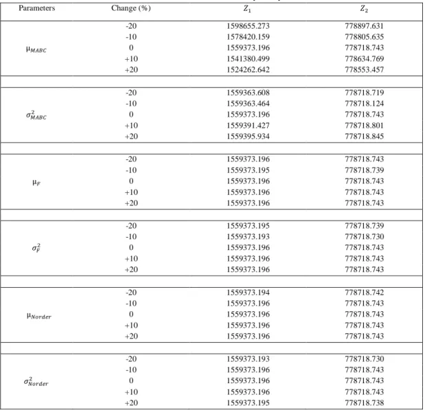
The first objective function (1) aims to minimize the total cost of VMI chain including ordering cost, holding cost, fixed and linear backordering costs and unused storage space cost, respectively. The second objective in Equation (11) aims to minimize the total amounts of GHGs emissions, including the amounts of greenhouse gases emissions in holding products in warehouse and the amounts of greenhouse gases emissions in transporting products by trucks from vendor to buyer, respectively. Equation (12) is a stochastic backordering costs constraint, where we assume that the backordering costs follow a normal distribution with mean µ𝑀𝐴𝐵𝐶 and standard deviation 𝜎𝑀𝐴𝐵𝐶. To put it another way, this constrain becomes:

∑ (

𝜋2𝑏𝑗2

2𝑄𝑗(1 −

𝐷𝑗

𝑃𝑗)

)

𝑗∈𝐽

+ 𝑍𝛼𝜎𝑀𝐴𝐵𝐶 ≤ µ𝑀𝐴𝐵𝐶

(22)

Where, 𝑍𝛼is the upper 𝛼-percentile point of the standard normal distribution. In equation (13) storage space constraint is considered stochastic, because in some cases, the supplier tends to lease warehouse to storage his products, but there may be uncertainty in the amount of storage space for storing products or the supplier may be the owner of the warehouse and tends to produce other products and store them in storage, in addition to the current products or he may be desirable to use part of the warehouse space for other activities, such as production besides storing products, there are uncertainty in the above conditions. Therefore, the storage space constraint can be considered stochastic, and similar to the previous constraint it becomes:

∑ (𝑓𝑗𝑄𝑗(1 −

𝐷𝑗

𝑃𝑗

) − 𝑏𝑗) 𝑗∈𝐽

+ 𝑍𝛼𝜎𝐹 ≤ µ𝐹

(23)

In equations (14) and (15) budget and the number of orders constraints are considered stochastic and similar to equation (12) we have:

∑(𝐶𝑗𝑄𝑗) 𝑗∈𝐽

+ 𝑍𝛼𝜎𝐵𝑢𝑑𝑔𝑒𝑡 ≤ µ𝐵𝑢𝑑𝑔𝑒𝑡 (24)

∑ (𝐷𝑗 𝑄𝑗

)

𝑗∈𝐽

+ 𝑍𝛼𝜎𝑁𝑜𝑟𝑑𝑒𝑟≤ µ𝑁𝑜𝑟𝑑𝑒𝑟

(25)

Equation (16) indicates the bounds on the buyer’s order quantity of product 𝑗. Equation (17) ensures that the maximum backorder level of product 𝑗 in a cycle should be equal or less than the quantity of the buyer's orders. Equation (18) guarantees that 𝑗th product carried by 𝑚 trucks should be more than or equal to the buyer's order quantity of product 𝑗. Equation (19) indicates the limited capacity of trucks. Equations (20) and (21) limit the decision variables of the model. The goal is to find the economic order quantity of product 𝑗 (𝑄𝑗), the maximum backorder level of product 𝑗 (𝑏𝑗), and the

(12)

12

total amount of product 𝑗 shipped by truck 𝑖 (𝑍𝑖𝑗), in a cycle of VMI chain, such that the total cost of the VMI chain in the first objective described in equation (10), and the total greenhouse gases emissions in the second objective function given in equation (11) are minimized, while the model constraints are satisfied.

5- The proposed solution methods

In numerous decision-making problems in real environment, we will be faced with a variety of goals and criteria, and all these goals and criteria could be proposed in the multi-criteria decision making space. A multi-objective optimization problem is a subset of a multi-criteria decision making in an uncountable (continuous) space. The proposed model in section 4.5 is a constrained multi-objective problem. Multi-objective problems are relevant to the optimization of multiple (vector of objectives), conflicting, and incommensurable objective functions issue to limit exposing the application of multi-objective optimization problems. Since both multi-objective functions aim to minimize the problem, the multi-objective optimization problem can be formulated as follows:

min {𝐹1(𝑥), 𝐹2(𝑥), … , 𝐹𝑘(𝑥)} (26)

𝑋



𝑅𝑛 ₍₂₇₎

Subject to:

𝑋



𝑥 (𝑋 is a feasible set; 𝑋 is unrestricted in sign) (28)

𝑘 ≥ 2 (The number of objectives) (29)

Where 𝑘 determines the number of objectives by assuming that 𝑘 is equal or more than 2, and the set 𝑥 is the feasible set of decision vectors. In order to optimize different and sometimes conflicting objective functions simultaneously, there are two general approaches: It can be used by combining the values of different objective functions and obtaining a fitness value, and eventually converting the problem into a single-objective function, or it is possible to use Pareto optimal solution to obtain answers that optimize the objective functions in a way that guarantee the rationality of a decision. There are different methods to solve multi-objective optimization problems such as multi-objective decision making (MODM) techniques, non-dominated sorting genetic algorithm-II (NSGA-II), multi-objective particle swarm optimization (MOPSO), strength Pareto evolutionary algorithm (SPEA-2), etc. In this research, MODM techniques are used to convert the multiple objectives into a single objective optimization problem.

5-1- MODM techniques

Generally, approaches used in multi-objective decision-making methods are based on the time and type of information received from decision makers, and are classified into four categories: in the first category, there are methods that don't receive information from decision makers during the resolution process, the LP metrics, global criteria, the Maxi-Min and the Filtering/displaced ideal solution (DIS) are placed in this category. The approach used in the second category consists of the goal programming, the lexicography/preemptive optimization, converting objectives into constraints, the goal attainment and the utility function that begins by getting initial information from the decision maker before solving the problem. In the third category, the analyst obtains information from the decision maker, interactively during the problem solving process, including Geoffrion method and satisfactory goals method. In the fourth category information, the preferences of decision maker for different solution methods will be achieved at the final stages of the resolution process, consists of the multi-criteria simplex method, the minimum deviation method, and the De Novo programming. In this section, there are three multi objective decision making (MODM) techniques, including LP-metrics, Goal attainment and Multi-choice goal programming with utility function. All of these methods are solved by a non-linear programming solver (i.e., Baron Solver) in Gams software.

5-1-1- Goal attainment

In this section, goal attainment method of Gembicki (1994), which is the modified form of the goal programming method is utilized to solve the multi-objective problem. In this technique, similar to the

(13)

13

goal programming method, the desirable solution is affected by the vector of goal and the vector of weighting specified by the decision maker. In contrast to the interactive multi-objective methods, Goal attainment technique is a one-stage approach which works with fewer variables. Thus, compared to other methods, this method has less computational complexity. Consequently, due to the high capability of this method in terms of computational time, it is one of the best MODM methods to solve our green VMI supply chain problem in the form of nonlinear program. Goal attainment technique has been successfully implemented to solve a number of real-world multi-objective optimization problems in reliability optimization (Azaron et al., 2007a), project management (Azaron et al., 2007b) and production systems (Azaron et al., 2006), and we use this technique to solve the stochastic green VMI supply chain problem. This method demonstrates a set of designed goals 𝐹∗₌

{𝐹₁∗_{, 𝐹}

2∗, … , 𝐹𝑘∗} which is associated with a set of objectives, 𝐹(𝑥) = {𝐹1(𝑥), 𝐹2(𝑥), … , 𝐹𝑘(𝑥)}. This method involves setting up a goal and weight, 𝑏𝑖 and 𝑤𝑖 (𝑤𝑖 ≥ 0), for 𝑖=1,2, for the two introduced objective functions. The 𝑤𝑖 described the relative under-attainment of the 𝑏𝑖. For under-attainment of the goals, a smaller 𝑤𝑖 is related to the more significant objectives. When 𝑤𝑖 reaches 0, then the objective function associated with, must be fully satisfied or the associated objective function value should be less than or equal to its goal 𝑏𝑖. The general mathematical formulation of this method obtained by:

min 𝑍 (30)

Subject to:

𝐹𝑖(𝑥) − 𝑤𝑖𝑍 ≤ 𝑏𝑖 (31)

𝑖 = 1,2, … , 𝑘 (32)

𝑋



𝑥 (

x

is a feasible set; X is unrestricted in sign( (33)

𝑘 is the number of objectives, 𝐹𝑖(𝑥) is the 𝑖th objective function, 𝑍 is the free variable of the problem that indicates the maximum objective deviation from the goal and must be minimized, 𝑤𝑖 is the normalized weight of the 𝑖th objective function, so that ∑𝑘𝑖=1𝑤𝑖 = 1, and 𝑏𝑖 is the ideal solution for the 𝑖th objective function. In fact, this method is a min-max method that minimizes the maximum objective deviation from the goal. The optimal solution using this formulation is sensitive to 𝑏 and 𝑤. According to the values for 𝑏, it is possible that the optimal solution is not influenced remarkably by

𝑤.

5-1-2- Multi-Choice Goal Programming with Utility Function (MCGP-U)

We use multi-choice goal programming with utility function (MCGP-U) technique, which is a combination of Choice Goal programming and utility function approaches to solve the multi-objective problem presented by Chang (2011) for the first time. This method, presented a novel theory of level achieving in the utility functions to substitute the aspiration level with scalar value in classical goal programming (GP) and multi-choice goal programming (MCGP) for multiple objective problems. Also, this method can be used as measuring tools to give assistance to decision makers make the best/suitable policy associated with their goals with the highest level of utility obtained. Moreover, it can improve the practical utility of MCGP in solving more real-world decision/management problems. It is for the first time that we use this technique to solve a multi-objective stochastic green VMI supply chain problem. In this method, according to the type of objective functions of problem, left linear utility function (LLUF) and right linear utility function (RLUF) are used. In this research based on the objective functions, we use LLUF to formulate MCGP-U. Therefore, we have:

min 𝑍 = ∑[𝑤𝑖(𝑑𝑖++ 𝑑𝑖−) + 𝛽𝑖𝑓𝑖−] 𝑘

𝑖=1

(34)

Subject to:

𝜆𝑖 ≤

𝑔𝑖,𝑚𝑎𝑥− 𝑦𝑖

𝑔𝑖,𝑚𝑎𝑥− 𝑔𝑖,𝑚𝑖𝑛

𝑖 = 1,2, … , 𝑘 (35)

𝑓𝑖(𝑥) − 𝑑𝑖++ 𝑑𝑖−= 𝑦𝑖 𝑖 = 1,2, … , 𝑘 (36)

𝑔𝑖,𝑚𝑖𝑛 ≤ 𝑦𝑖 ≤ 𝑔𝑖,𝑚𝑎𝑥 𝑖 = 1,2, … , 𝑘 (37)

(14)

14

𝑑_𝑖+, 𝑑_𝑖−, 𝑓_𝑖−, 𝜆𝑖≥ 0 𝑖 = 1,2, … , 𝑘 (39)

𝑋



𝑥 (𝑥 is a feasible set; 𝑋 is unrestricted in sign( (40)

Where 𝑑_𝑖+ and 𝑑_𝑖− are the positive and negative deviations attached to the 𝑖th goal. 𝑤𝑖 and 𝛽𝑖 are weights attached to deviations 𝑑_𝑖+, 𝑑_𝑖−and 𝑓_𝑖−. 𝑦𝑖 is the continuous variable with a range of interval values 𝑔𝑖,𝑚𝑖𝑛 ≤ 𝑦𝑖 ≤ 𝑔𝑖,𝑚𝑎𝑥, 𝑔𝑖,𝑚𝑎𝑥 and 𝑔𝑖,𝑚𝑖𝑛 are the upper and lower bounds of 𝑦𝑖. 𝜆𝑖 is the utility value of the 𝑖th goal and 𝑘 is the number of objective functions.

5-1-3- Linear Programming-metrics method (LP-metrics)

As the model proposed by current study is a multi-objective, non-linear programming model with conflicting objective functions, it was decided to apply the LP-metrics method that is useful and simple in execution introduced by Zeleny (1982), Duckstein & Opricovic (1980) and Szidarovszky et al. (1986). So far, several multi criteria decision making (MCDM) methods have been developed and investigated to solve multi-objective problems with inconsistent objective functions. One of the reasons we used the LP-metrics method is that LP-metrics approach is one of the well-known methods and widely used for solving the problems of this kind. In the Linear Programming (LP)-metrics method, a multi-objective problem is solved by optimizing each objective function separately, and then converting the problem to a single-objective optimization. By using LP-metrics method, the difference between any present solutions and the optimal solution are minimized (Branker et al., 2008). The mathematical formulation of this method is defined by:

𝑚𝑖𝑛 𝑍 = (∑ 𝑤𝑖|

𝐹𝑖(𝑥) − 𝐹𝑖∗

𝐹_𝑖∗ |

𝑝 𝑘

𝑖=1

)

1/𝑝 ₍₄₁₎

Subject to:

𝑋



𝑥 For 1 ≤ 𝑝 ≤



(42) (𝑥 is a feasible set; 𝑋 is unrestricted in sign(

𝑘 represents the number of objective functions, 𝐹𝑖(𝑥) is the 𝑖th objective function, 𝐹𝑖∗ presents the ideal solution for optimizing the 𝑖th objective function. 0 ≤ 𝑤𝑖 ≤ 1 (∑𝑘𝑖=1𝑤𝑖 = 1) represents the relative weight of components involved in the objective function (Mirzapour et al., 2011). The value of 𝑤𝑖 are given by decision maker’s measures. 𝑝 is a parameter that controls the deviation of the objective function from the ideal solution. There are different values for 𝑝. values 1, 2 or ∞ are usually considered for it. The value of 𝑝 demonstrates the type of metric. For 𝑝=1, we obtain the Manhattan metric and for 𝑝=∞, we obtain the Tchebycheff metric. In this study, we consider 𝑝=1. Whatever the amount of 𝑝 is considered lower, the problem shows the lower sensitivity to the difference from the optimal level. According to the above mathematical formulation mentioned, single objective function of our model (𝑍) can now be formulated by:

𝑚𝑖𝑛 𝑍 = 𝑤1×

𝐹1− 𝐹1∗

𝐹₁∗ + 𝑤2×

𝐹2− 𝐹2∗

𝐹₂∗

(43) By considering this single objective function and our model constraints, a single-objective, non-linear programming model can be acquired and solved by a non-non-linear programming solver (i.e., Baron Solver) in Gams software. It is noted that the 𝐹1 and 𝐹2 minimize the first and second objective functions, respectively. 𝐹1∗ and 𝐹2∗ are the ideal solution for optimizing the first and second objective functions, respectively. 𝑤1 and 𝑤2 represent the relative weights of the first and second objective functions, respectively.

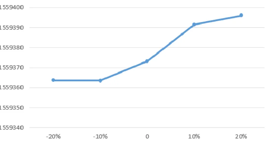
6- Computational results, comparisons and sensitivity analysis

In this section, first, three mentioned approaches are implemented on a set of 30 test problems, and then are compared in terms of the three comparison criteria, including the first objective function, the second objective function, and computational time (CPU time). Afterward, statistical analysis and MCDM approach that aim to specify significant differences among the proposed algorithms are applied. Finally, sensitivity analysis is investigated.

(15)

15

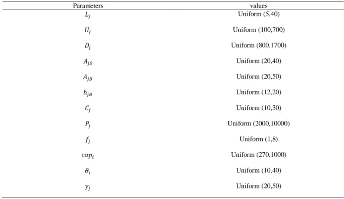
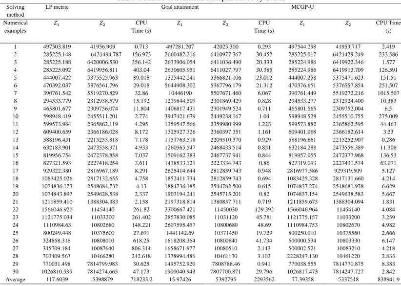
6-1- Comparison results

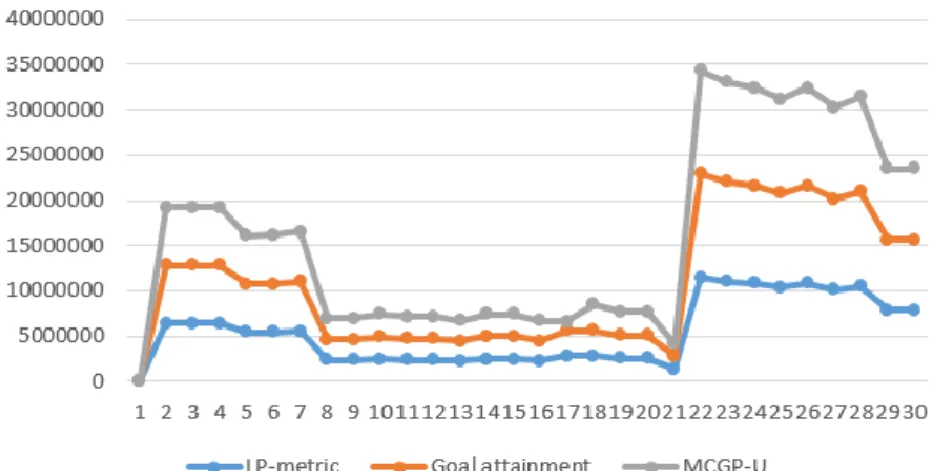
Referring to Roozbeh Nia et al. (2015), different dimensions and parameter values of the numerical example are used to solve the model presented in table 2 and table 3, respectively. It should be noted that we use uniform distribution to produce data in table 3. In order to evaluate and compare three proposed methods, 30 test problems in different sizes are designed and three mentioned methods are implemented to obtain solutions in terms of three considered evaluation criteria that shown in table 4. The results in this table show that in average, LP-metrics, MCGP-U, and Goal attainment have the best performance in terms of the first objective function, the second objective function, and CPU time criteria, respectively. Note that the solving methods are implemented using GAMS/Baron software (win32, 24. 1. 2) on a pc with 2.2 GHz Intel Core 2 Duo CPU, and 4 GB of RAM memory. In addition, the performance of methods in the first and second objective function and CPU time is shown in figures 1, 2, and 3, respectively.

Table 2. Numerical examples with different dimensions

Numerical examples 𝑖, 𝑗 Numerical examples 𝑖, 𝑗

1 20,60 16 10,55

2 20,50 17 10,55

3 20,90 18 10,55

4 20,90 19 10,50

5 20,80 20 5,50

6 20,80 21 5,50

7 20,80 22 20,120

8 10,70 23 20,120

9 10,70 24 20,115

10 10,70 25 20,115

11 10,65 26 20,115

12 10,65 27 20,110

13 10,60 28 20,110

14 10,60 29 15,100

15 10,60 30 15,100

Table 3. Parameters and values

Parameters values

𝐿𝑗 Uniform (5,40)

𝑈𝑗 Uniform (100,700)

𝐷𝑗 Uniform (800,1700)

𝐴𝑗𝑆 Uniform (20,40)

𝐴𝑗𝐵 Uniform (20,50)

ℎ𝑗𝐵 Uniform (12,20)

𝐶𝑗 Uniform (10,30)

𝑃𝑗 Uniform (2000,10000)

𝑓𝑗 Uniform (1,8)

𝑐𝑎𝑝𝑖 Uniform (270,1000)

𝜃𝑖 Uniform (10,40)

(16)

16

Table 4. Results of numerical examples solved by GAMS Solving

method

LP metric Goal attainment MCGP-U

Numerical examples

𝑍1 𝑍2 CPU

Time (s)

𝑍1 𝑍2 CPU

Time (s)

𝑍1 𝑍2 CPU Time (s)

1 497503.819 41956.909 0.713 497281.207 42023.300 0.293 497544.298 41953.717 2.419 2 285225.148 6421494.787 156.973 2660482.216 6410977.367 30.452 285225.017 6421429.249 233.586 3 285225.188 6420006.530 356.142 2633906.054 6411036.490 20.333 285224.986 6419922.346 1.577 4 285225.092 6419956.811 403.04 2630605.951 6411027.797 30.385 285224.986 6419913.709 126.591 5 444007.422 5375525.963 89.018 1325442.241 5366821.106 23.012 444007.258 5375471.623 151.51 6 470392.037 5376561.796 29.018 5644908.302 5367796.179 21.312 470376.651 5376557.854 251.507 7 390761.542 5519270.829 32.86 10446190 5507671.460 6.067 390761.449 5519272.216 1015.507 8 294533.779 2312938.579 15.192 1239844.509 2301869.429 0.828 294533.277 2312924.400 10.383 9 465801.677 2309756.074 11.804 1406817.431 2301949.524 0.711 465801.565 2309752.004 6.5 10 598948.419 2455511.201 2.774 3947421.679 2449238.167 1.04 598948.528 2455510.755 275.009 11 599573.964 2365862.119 4.295 1359547.566 2359980.999 1.223 599573.882 2365862.595 44.463 12 609400.659 2366186.028 8.172 1325927.326 2360397.351 1.161 609401.068 2366182.614 3.23 13 588196.451 2215253.818 7.178 1151763.518 2209510.370 0.929 588196.661 2215252.907 0.286 14 632183.901 2473558.371 4.933 1260565.547 2468433.514 0.851 632184.288 2473556.389 11.308 15 819956.754 2472378.858 7.037 1509162.383 2467737.941 0.844 819957.055 2472377.968 136.53 16 827321.593 2227418.254 3.611 1438533.321 2223334.743 0.86 827319.093 2227431.574 63.071 17 929322.380 2816967.189 8.291 2625414.644 2812859.743 0.948 2816977.586 929319.509 5.127 18 1083425.026 2817132.655 4.758 1852411.734 2812859.743 0.694 1083425.328 2817131.660 4.214 19 1074836.123 2548684.732 4.13 1884736.185 2544782.500 0.615 1074837.274 2548681.978 6.629 20 1074843.897 2549628.538 2.337 1903194.241 2545715.201 0.82 1074837.154 2549638.583 5.667 21 1211859.410 1388304.383 2.158 2197318.814 1380857.711 0.719 1211859.675 1388304.094 1.831 22 1566046.920 11454140 261.82 3300667.421 11450030 129.392 1566046.964 11454140 4.084 23 1121775.034 11033200 261.402 2857830.085 11031120 45.781 1121775.157 11033200 3.259 24 1110984.63 10802680 148.221 2607595.457 10800680 48.69 1110984.753 10802670 4.982 25 800249.448 10375600 27.691 1441142.69 10371450 19.729 800250.010 10375560 2.666 26 324858.316 10808010 618.25 1618208.364 10800640 41.734 500000.534 10803330 6.147 27 345709.184 10087640 806.314 1658671.977 10080510 2.143 500002.521 10083210 4.218 28 703409.567 10466280 242.618 1378994.486 10461130 3.103 2228247.130 10461220 2.833 29 770031.498 7814799.983 30.625 1495752.920 7808788.46 0.941 770038.555 7814770.875 8.383 30 1026810.535 7814274.665 47.173 1900040.943 7807700.871 29.796 1026817.473 7814247.727 2.842 Average 117.6039 5398879 718233.2 15.97426 5392795 2293562 77.39358 5337518 838941.9

Fig 1. Results of LP-metrics, Goal attainment and MCGP-U methods in first objective function

(17)

17

Fig 2. Results of LP-metric, Goal attainment and MCGP-U methods in second objective function

Fig3. Results of LP-metric, Goal attainment and MCGP-U methods in CPU time (s)

6-1-1- Comparison based on MADM technique

In this section, the technique for order preference by similarity to ideal solution (TOPSIS) is employed to compare three solving methods by using the first objective function, the second objective function and CPU time criteria, in order to find a method with the best performance.

6-1-1-1- The technique for order preference by similarity to ideal solution (TOPSIS)

The technique for order preference by similarity to ideal solution which first was introduced by Hwang & Yoon (1981) and developed by Yoon (1987) and Hwang et al. (1993), is one of the multi-criteria decision-making methods which is used to rank a set of alternatives, and choose the best alternative which havethe farthest distance from the negative-ideal solution and the shortest distance from the positive-ideal solution. Positive-ideal solution seeks to minimize the cost criteria or maximize the profit criteria.On the other hand, the negative-ideal solutionseeks to maximize the cost criteria or minimize the benefit criteria. The TOPSIS method consists of six steps which are explained below.

(18)

18

Table 5. The means of results prepared by algorithms

𝑍1 𝑍2 CPU time (s)

LP-metric 718233.2 5398879 117.6039

Goal attainment 2293562 5392795 15.97426

MCGP-U 838941.9 5337518 77.39358

1. The first step

To compare the alternatives LP-metrics, Goal attainment and MCGP-U, the means of four criteria presented in table 5, should be normalized using Euclidean norm which calculated in equation (44).

𝑛𝑖𝑗 =

𝑟𝑖𝑗

√∑3_𝑖=1𝑟_𝑖𝑗2

2

𝑗 = 1,2,3 (44)

Where 𝑖 and j are the indices related to the alternatives and attributes, respectively. 𝑛𝑖𝑗 is a normalized score for 𝑖th alternatives and jth attributes, 𝑟𝑖𝑗 is the score for the 𝑖th alternatives, according to the 𝑗th attributes. The normalized values are presented in table 6.

Table 6. The normalized values

LP-metric 0.282146273 0.579756846 0.830017474 Goal attainment 0.900988662 0.579103518 0.112742136 MCGP-U 0.32956473 0.573167615 0.546223584

2. The second step

According to the weights assigned to the attributes in table 7, the normalized scores are weighted, in which the equal weights are considered for three attributes.

Table 7. The weighted normalized values

LP-metric 0.094048758 0.193252282 0.276672491 Goal attainment 0.300329554 0.193034506 0.037580712 MCGP-U 0.10985491 0.191055872 0.182074528

3. The third step

Positive-ideal and negative-ideal solutions are calculated based on the normalized weighted values, so that 𝐴+=[0.094048758, 0.191055872, 0.037580712]is the best value of thejth attribute among all alternatives and 𝐴−_{=[0.300329554, 0.193252282, 0.276672491] is the worst value of the}_j_{th attribute} among all alternatives.

4. The fourth step

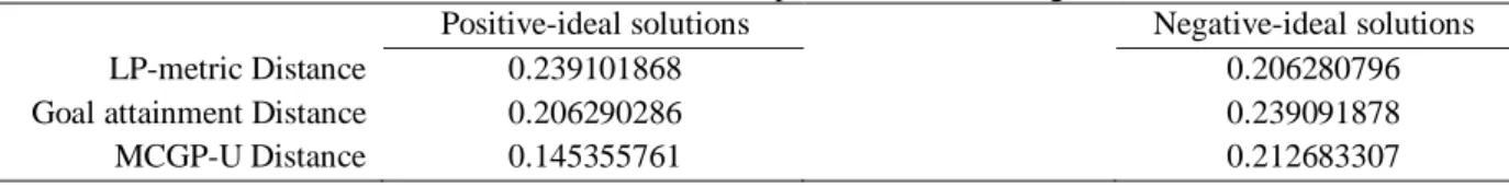
The Euclidean distances of each alternative from the positive-ideal and negative-ideal solutions are shown in table 8 which calculated as follows:

𝑑𝑖+= √∑(𝑣𝑖𝑗− 𝑣𝑗+) 2 3

𝑗=1

(19)

19

𝑑𝑖−= √∑(𝑣𝑖𝑗− 𝑣𝑗−) 2 3

𝑗=1

𝑖 = 1,2,3 (46)

Where, 𝑑_𝑖+ is the Euclidean distances of each alternative from the positive-ideal solutions, 𝑑_𝑖− is the Euclidean distances of each alternative from the negative-ideal solutions, 𝑣𝑖𝑗 is the normalized weighted values, 𝑣𝑗+ is the vector of the best values of each attribute, and 𝑣𝑗− is the vector of the worst values of each attribute.

Table 8. The distance of alternatives from the positive-ideal and negative-ideal solutions

Positive-ideal solutions Negative-ideal solutions

LP-metric Distance 0.239101868 0.206280796

Goal attainment Distance 0.206290286 0.239091878

MCGP-U Distance 0.145355761 0.212683307

5. The fifth step

Finally, in order to rank alternatives, the closeness index (𝐶𝐿+_{) for each alternative is calculated in} table 9 by using equation (47).

𝐶𝐿+= 𝑑𝑖− 𝑑_𝑖−+𝑑_𝑖+

(47)

𝐶𝐿+ determines the closeness of each alternative from the ideal solution, so the alternative with the highest 𝐶𝐿+_{has the best performance and should be selected as the best alternative. As}_𝐶𝐿+_for LP-metrics, Goal attainment and MCGP-U are 0.463154, 0.536824, and 0.594023, respectively, it can be concluded that MCGP-U has better efficiency than Goal attainment and LP-metrics, and Goal attainment has better performance than LP-metrics. It should be noted that bigger values of the three mentioned criteria are preferred.

Table 9. Results of TOPSIS method

LP-metrics Goal attainment MCGP-U

TOPSIS 0.463154 ≤ 0.536824 ≤ 0.594023

6-1-2- Statistical analysis

In this section, the differences between the three presented methods in terms of the means of the employed criteria are statistically investigated. For each criterion, a single-factor analysis of variance (ANOVA) is utilized to test the equality of the means of criterion gained by the methods against the inequality of the means in order to specify whether there are significant differences between the solution methods in terms of the employed criteria when the standard deviations are uncertain. In each experiment, the two hypotheses are:

{𝐻_𝐻0: µ1= µ2= µ3

1: µ1≠ µ2≠ µ3

(48)

On the one hand, the null hypothesis in (48), representing the equality of the means of the methods in terms of a particular criterion, indicates no significant differences between them. On the other hand, the opposite situation is speculated by alternative hypothesis in (48). In this paper, the MINITAB software is employed to execute the Tukey’s test. Three ANOVA experiments are designed according to the data results in Table 4, each for one criterion.

6-1-2-1- First objective function criterion

Table 10 provided the outputs of the single-factor analysis of variance by the Tukey’s multiple comparison tests for the first objective function (𝑍1) criterion.

(20)

20

Table 10. Single-factor analysis of variance by the Tukey’s multiple comparison tests for the first objective function criterion

Source DF Adjusted SS Adjusted MS F-value p-value Test result Method 2 4.74418×1013

2.37209×1013 _18.71 _0.000 _null Error 87 1.10292×1014 _1.2677×₁₀12 _---- _---- _hypothesis Total 89 1.57734×1014 _---- _---- _---- _{is rejected}

Confidence level = 95%

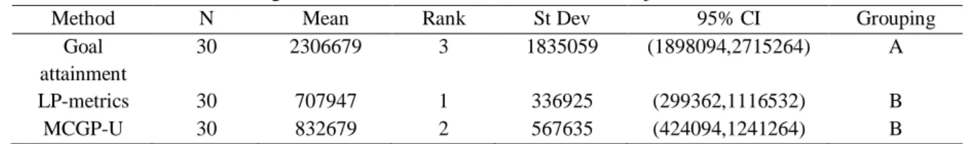
According to table 10, the p-value resulted from ANOVA, is less than 0.05. This implies that null hypotheses of equality of the first objective function is rejected at 95% confidence level, and significant differences are existed between the performances of LP-metrics, Goal attainment and MCGP-U methods in terms of the first objective function. In this case, when the solution methods generate significantly different outcome, in order to find out how the solution methods vary from each other, a post hoc analysis, such as the Tukey’s multiple comparison test is performed (Montgomery et al., 1973). Table 11 displays the ranking of the solution methods in terms of the first objective function,according to the results of Tukey’s test.

Table 11. Ranking the solution methods in terms of the first objective function criterion

Method N Mean Rank St Dev 95% CI Grouping

Goal attainment

30 2306679 3 1835059 (1898094,2715264) A

LP-metrics 30 707947 1 336925 (299362,1116532) B

MCGP-U 30 832679 2 567635 (424094,1241264) B

According to the results obtained by table 11, LP-metrics and MCGP-U are in the same group and Goal attainment is different from them. That means there is no significant difference between the LP-metrics and MCGP-U in terms of the first objective function, but significant differences are existed between the Goal attainment and two other solution methods in terms of the first objective function. Also, since lower value of the first objective function is preferred, the results of table 11 indicate that LP-metrics has remarkably the best performance in terms of the first objective function criterion among the mentioned solution methods. The results of the Tukey’s multiple comparison tests in an analogical manner are expressed in figures 4 and 5. Figure 4 depicts the lower and upper limits of the criteria generated by each solution method presented in box plots. Basically, if the boxes do not cross each other, a significant difference is existed between the solution methods. According to figure 4, since significant overlap exists between the boxes related to LP-metrics and MCGP-U, there is no significant difference between them, but, as no overlap is observed between the boxes of the Goal attainment and two other mentioned solution methods, significant differences are existed between the Goal attainment and two other mentioned solution methods in terms of the first objective function criterion. According to figure 5, if an interval does not contain zero, the corresponding methods are significantly different. As a result, Goal attainment is significantly different from LP-metrics and MCGP-U in terms of the first objective function criteria, but there is no significant difference between LP-metrics and MCGP-U in terms of the first objective function criterion. It can be concluded that LP-metrics and MCGP-U are in the same group.

(21)

21

Fig 4. Boxplot of the average of the first objective function of the solution methods

Fig 5. Tukey’s simultaneous 95 percent intervals for the first objective function comparison

6-1-2-2- Second objective function criterion

Table 12 provided the outputs of the single-factor analysis of variance by the Tukey’s multiple comparison test for the second objective function (𝑍2) criterion.

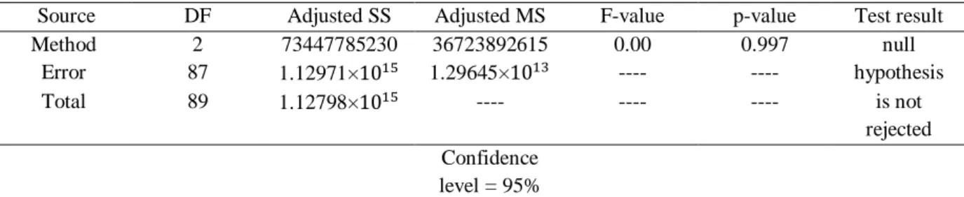
Table 12. Single-factor analysis of variance by the Tukey’s multiple comparison tests for the second objective function criterion

Source DF Adjusted SS Adjusted MS F-value p-value Test result

Method 2 73447785230 36723892615 0.00 0.997 null

Error 87 1.12971×1015 _1.29645×₁₀13 _---- _---- _hypothesis

Total 89 1.12798×1015 _---- _---- _---- _{is not}

rejected Confidence

level = 95%

According to table 12, the p-value resulted from the ANOVA is more than 0.05, expressing that null hypotheses of equality of the first objective function is not rejected at 95% confidence level, and significant differences are not existed between the performances of LP-metrics, Goal attainment and

(22)

22

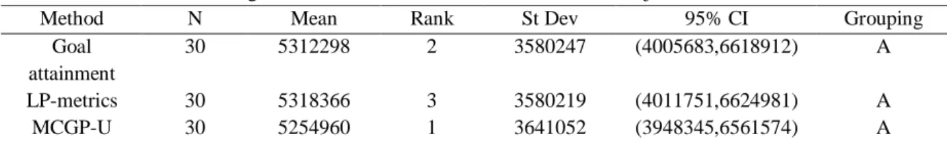
MCGP-U methods in terms of the second objective function. Table 13 displays the ranking of the solution methods in terms of the second objective function,according to the results of Tukey’s test.

Table 13. Ranking the solution methods in terms of the second objective function criterion

Method N Mean Rank St Dev 95% CI Grouping

Goal attainment

30 5312298 2 3580247 (4005683,6618912) A LP-metrics 30 5318366 3 3580219 (4011751,6624981) A

MCGP-U 30 5254960 1 3641052 (3948345,6561574) A

Based on the results obtained by table 13, all of the solution methods are in the same group and that means there is no significant difference between them. Also, since lower value of the second objective function is preferred, the results of table 13 indicate that MCGP-U has remarkably the best performance in terms of the second objective function criterion among the mentioned solution methods. Figures 6 and 7 express the results of the Tukey’s multiple comparison tests in an analogical manner. According to figure 6, since the boxes cross each other, a significant difference is not existed between the solution methods. According to figure 7, since an interval contains zero, there is no significant difference between the three methods in terms of the second objective function criterion.

Fig 6. Boxplot of the average of the second objective function of the solution methods

Fig 7. Tukey’s simultaneous 95 percent intervals for the second objective function comparison 6-1-2-3- CPU time criterion

Table 14 provides the outputs of the single-factor analysis of variance by the Tukey’s multiple comparison tests for the CPU time criterion.