A MinMax Routing Algorithm for Long Life Route Selection in MANETs

A MinMax Routing Algorithm for Long Life

Route Selection in MANETs

Abdorasoul Ghasemi

Tehran, Iran [email protected]

Mahmood Mollaei

Tehran, Iran [email protected]

Received: May 10, 2015- Accepted: August 28, 2015

Abstract— In this paper, the stable or long life route selection problem in Mobile Ad-hoc Wireless Networks (MANETs) is addressed. The objective is to develop an on demand routing scheme to find a long life route between a given source and destination assuming each node has an estimate of neighbors’ mobilities. Formulating the problem as a MinMax optimization one, we use a dynamic programming based scheme for route selection. The proposed MinMax Routing Algorithm (MRA) is an on demand routing that can be implemented in the traditional Ad-hoc On-Demand Distance Vector (AODV) structure. In the route request phase, tail subproblems of finding the most stable route from the source to each intermediate node are solved. MRA finds the most stable route in the route reply phase deploying the solutions of these subproblems. Simulation results using NS2 simulator are provided to show the performance of MRA compared to AODV and stable AODV schemes in terms of the lifetime of selected route and routing overhead. Also, the tradeoff between the route discovery delay and finding more stable routes is discussed and justified by simulations.

Keywords- Mobile ad-hoc network; routing; route stability; ad-hoc on-demand distance vector; dynamic programming.

I. INTRODUCTION

A Mobile Ad-hoc Network (MANET) is a wireless network which consists of mobile nodes with dynamic topology. The routing problem in MANETs has remained as a challenging topic in the researches of recent years. The purpose of routing is to find a proper route between a source and destination considering some predefined metrics and constraints. Routing overhead, delay, throughput and route’s stability can be regarded as the most important metrics in routing [1].

Proactive and reactive schemes are two important classes of routing protocols for wireless ad-hoc networks. In proactive protocols, routes are computed regardless of the possible sources and destinations which may use them in future. However, in reactive or on demand protocols routes are computed when a

communication between a source and destination is required [2]. While, proactive protocols have less route discovery delay, they incur higher overhead especially when the nodes are mobile. Therefore, for MANETs with dynamic topology the reactive protocols are more scalable and hence interesting. Dynamic Source Routing (DSR) and Ad-hoc On-Demand Distance vector (AODV) are the most famous and wildly used protocols in this class [2]. AODV discovers and establishes a route before sending data to the destination. The route which has the minimum number of hops to the destination is selected and considered as the optimal one.

In AODV, the source node broadcasts the Route Request (RREQ) packet in order to initiate route discovery process if there is no route entry to the destination in its table. RREQ contains the source and destination addresses, source and destination sequence

numbers, broadcast id and hop count field [3]. Both

sequence number and broadcast id are implemented as

in each node and is incremented when a new RREQ is broadcasting. A node which receives the RREQ may drop, broadcast or reply with Route Reply (RREP) packet. That is, if the node is the destination or knows a fresh route to the destination, it unicasts a RREP packet to the RREQ sender. If the node has already received an identical RREQ packet from other neighbors, it drops the packet to restrict the broadcast region. Otherwise, the node rebroadcasts the RREQ packet and keeps the RREQ field in a table for reverse path to the source node. The source node starts transmitting data packets when the RREP arrived.

Nodes' mobility leads to two main problems including link failure and changing in the computed optimal path. Link failure is reported by a Route Error (RERR) packet from the uplink node of the broken link in active route. In such cases, the source attempts to discover a new route toward the destination.

To avoid route errors and extra overhead, it is strongly desired to select long life or stable routes in the route discovery phase of reactive protocols. The key factor which determines the link stability in MANETs is the mobility of nodes. Since the characteristics of nodes’ movements are stochastic, finding a stable route in such networks is an interesting subject. The main challenge is to define a measure for link stability and then using this measure to characterize the route stability. It is worth to note that without using a plan for discovering a stable route between a source and destination, one needs an exhaustive search among all possible routes and this will force much overhead on the network.

In [4], an entropy based modeling is developed to address the nodes’ mobility effects on link stability. The relative mobility between a node and its adjacent nodes is deployed in a normalized entropy function to predict the link stability. The minimum or product of these local link measurements are considered as the route stability measure in [4]. Also, a probabilistic approach is used in [5] where the probability of route stability is determined under the assumption of random direction mobility model. Using the link stability measurements and optimum number of hops between a source and destination, the most stable route is selected in [5]. Furthermore, the self-content information is deployed in [6] to estimate a local link maintenance metric between two adjacent nodes.

In [7], the link lifetime is considered as the minimum of nodes’ lifetimes and the lifetime of connection. The former relates to the remaining energy of the nodes and the latter is determined by their mobility profiles. Authors in [7] also proposed a route lifetime prediction algorithm which can be implemented based on DSR. A random walk based mobility model is used in [8] to find the probability density function (PDF) for link stability. The product term of the probabilities of links’ stability is used to determine the corresponding route stability. Moreover, a new route stability computation model is developed using the correlation factor between adjacent links in [9]. This correlation shows the degree of dependency between links in a MANET.

In addition, the routing problem is formulated as an offline tractable optimization problem where the links’ costs and their durations are computed using an offline algorithm in [10].

The main challenge in finding a feasible and practical solution to the routing problem in a MANET is to find a stable route in term of link stability that can be implemented in the framework of existent routing protocols. In this paper, we propose a solution which jointly takes into account these criteria and has a reasonable time delay for route discovery as well. The implementation complexity of the proposed scheme for stable route selection is the same as AODV, and also, the stability of selected routes by this scheme is comparable with the recent proposed scheme in [11].

Also, some researchers have attempted to address the problem of sub optimality of the initial computed stable path due to nodes' mobility such as [12]. In [12], an “Event driven dynamic path optimization for AODV in MANET” is presented. In this scheme at first the route is established by AODV. If on active route two non-adjacent nodes become neighbors an event is triggered. Upon an event occurrence, the middle node initiates a new optimal path calculation by generating a proxy route request for each destination entry that it has in its routing table. This process increases the routing overhead dramatically.

We consider the routing algorithm as a sequential decision making problem where the objective is to find the most stable route using a proper link stability measurement. That is, starting from source, the sub problems of finding the most stable route to each intermediate node are computed in the route discovery phase. The route is then computed by using the solutions of these sub problems sequentially.

The rest of this paper is organized as follows. The system model and problem statement are presented in section II. In section III, we review some available metrics for link and route stabilities. Section IV discusses about a dynamic programming based algorithm for ad hoc routing as a sequential decision making problem. The MinMax model of the routing problem is presented in section V. Section VI includes the MinMax routing algorithm (MRA) for route selection and its performance is evaluated via simulations in section VII. Finally, the paper is concluded in section VIII.

II. SYSTEM MODEL AND PROBLEM STATEMENT Consider a MANET in which the set of nodes is denoted by 𝑁 = {𝑛1, … , 𝑛𝑁} where 𝑁is the total number of nodes. These nodes are uniformly distributed in a 𝐿 × 𝐿rectangular area and their transmission ranges are the same and equal to 𝑅𝑇. Two nodes are called neighbors if they are in the transmission ranges of each other. Let 𝑙𝑛_𝑖,𝑛_𝑗 denotes the link between 𝑛𝑖 and 𝑛𝑗 which is assumed to be symmetric.

The distributions of nodes’ mobility patterns are assumed to be independent and identically distributed. Also, Random Waypoint is considered as the mobility model of the nodes. That is, each node selects a random target in the network area and moves toward it

with a random velocity which is uniformly distributed in the range [0, 𝑉𝑚𝑎𝑥] . Before selecting another destination, the node pauses for a fixed duration of time that is called pause time [13].

The set of possible routes between a given source, 𝑆, and destination, 𝐷, is denoted by 𝑅 = {𝑅1, … , 𝑅𝑀} where 𝑀is the total number of routes between 𝑆 and 𝐷. The set of relaying nodes on route 𝑅𝑖 is shown by 𝑅𝑖= {𝑛1𝑖, 𝑛2𝑖, … , 𝑛𝑖𝑁_𝑖} where𝑛𝑘𝑖𝜖 𝑁, is the 𝑘𝑡ℎ relay node in the 𝑖𝑡ℎ _{route and 𝑁𝑖 is the total number of} relay nodes on this route. Furthermore, the set of links on route 𝑅𝑖 is denoted by 𝐿𝑖= {𝑙𝑛₁𝑖,𝑛₂𝑖, … , 𝑙𝑛

𝑁𝑖−1 𝑖 _,𝑛

𝑁𝑖𝑖 }.

It is assumed that 𝑙_𝑛

𝑗𝑖,𝑛𝑗+1𝑖 is active at time 𝑡 if the

distance between 𝑛𝑗𝑖 and 𝑛𝑗+1𝑖 are less than𝑅𝑇. The lifetime of a link, in general, is the time during which the link is active. Also, the route lifetime is defined as the time duration in which all the links in the route are active. The lifetime of the route 𝑅𝑖 and the link 𝑙_𝑛

𝑗 𝑖_,𝑛

𝑗+1

𝑖 𝜖 𝐿𝑖 are denoted by 𝑡𝑖 and 𝑡_𝑗𝑖, respectively.

The objective is to find the most stable route between 𝑆and 𝐷 in the network subject to a route discovery time delay. We use the cumulative distribution function (CDF) of the route lifetime to compare the results with other schemes. Also, we show the tradeoff between the route discovery delay and the probability of finding more stable routes.

III. LINK AND ROUTE STABILITY MEASURES

Route and link stabilities are related to each other because a good estimation of links’ lifetimes is a prerequisite to find a stable route. That is, deploying the local link stability measures a routing algorithm aims to find a global stable route between a source and destination. Given an estimation of links’ lifetimes, in this paper, we aim to find a routing algorithm that can be implemented in the framework of traditional routing protocols.

In this section, we first review two previously link stability criteria which can be deployed to construct a stable route. In following, we focus on our problem and argue about how to use these metrics for end to end route selection in MANETs. It should be mentioned that other link stability measures can be used in the proposed framework and formulation for stable end to end route selection.

A. Link Stability

In [8], a statistical model is developed to estimate the link stability, assuming that it is active at 𝑡0. The aim is to find the PDF of link stability in ∆𝑡 seconds after 𝑡0 . Also, it is assumed that the nodes’ transmission ranges are equal. Let 𝐴𝑗𝑖(∆𝑡) be the probability of finding node 𝑛𝑗𝑖 in the transmission range of node 𝑛𝑗+1𝑖 at 𝑡0+ ∆𝑡, on route 𝑅𝑖, if they were in the transmission range of each other at 𝑡0. It has been shown that the probability of finding this link stability for ∆𝑡 is given by [8]:

( 1 ) 𝐴𝑗𝑖(∆𝑡) = 1 − Φ (

1 2, 2,

−4𝑅_𝑇2 𝛼

𝑛𝑗𝑖 ,𝑛𝑗+1𝑖

) ; 𝛼𝑘,𝑚= 2∆𝑡(

𝜎_𝑘2+𝜇_𝑘2

𝜆_𝑘 +

𝜎_𝑚2+𝜇_𝑚2 𝜆_𝑚 )

Where Φ is the Kummer-confluent hypergeometric function, 1

𝜆𝑘is the mean of time epochs in mobility

model, and 𝜇𝑘 and 𝜎𝑘 are mean and variance of velocity of 𝑛𝑘, respectively. Therefore, having little information about the adjacent nodes, a node can predict the probability of finding its neighbors within Δ𝑡 seconds’ interval. For a given probability of link stability, the lifetime of each link in the network, can be calculated. Another approach to define the link lifetime is to measure the approximate time that a node will be available for its neighbors. In [14], this is approximated by:

( 2 ) 𝑡𝑗𝑖=

−(𝑎𝑏+𝑐𝑑)+√(𝑎2_+𝑐2_)𝑅 𝑇

2_{−(𝑎𝑏−𝑐𝑑)}2

(𝑎2_+𝑐2)

Where 𝑎 and 𝑐 are the relative velocity of 𝑛_𝑗𝑖 _and 𝑛𝑗+1𝑖 in 𝑥 and 𝑦 axes, respectively. Also, 𝑏 and 𝑑 are the relative location of the two nodes in 𝑥 and 𝑦 axes, respectively.

A time based link stability measure which is introduced in [11], defines link duration or link life time as the link stability measure. Sending Hello messages is the sign of presence of each node to its neighbors. Therefore, this measure is closely related to transmission interval of Hello messages. Note that, decreasing this interval will lead to increase the accuracy of this measure. However, it has adverse effect on overhead. The authors modify AODV protocol and simulate their approach using NS2 [15] and compare it with AODV as benchmark. In this paper, we use (2) as the link stability measure and the proposed algorithm is compared with [11] and traditional AODV.

B. Route Stability

Finally, given the links’ stability measures, greedy algorithm is the simplest scheme for link selection to find a stable route. In this scheme, deploying the mobility profiles, each node selects the most stable link in its neighborhood. It is obvious that this myopic scheme does not necessarily result in a stable route. In [8], the product of the links’ stabilities measures is considered as the route stability. Therefore, using (1), the route stability is computed by:

( 3 ) Pr(𝑃𝑖(𝑡0+ Δ𝑡) = 1|𝑃𝑖(𝑡0) = 1) = ∏ 𝐴𝑗𝑖(𝑡0+ Δ𝑡)

𝑁_𝑖−1 𝑗=1

Where 𝑃𝑖(𝑡0) = 1 indicates that 𝑅𝑖 is available atΔ𝑡. That is, the conditional probability of route existence at 𝑡0+ Δ𝑡 given that it is available at 𝑡0 is given by (3).

Therefore, the destination will select the most stable route between S and D if the links stability measures for all possible routes between these nodes are available. However, in a practical scenario, collecting this information incurs much overhead in the network.

In the following, we formulate the problem as a sequential decision making problem. The objective is to find a stable route taking into account the required overhead and simple implementation in the framework of a typical ad-hoc routing protocol like AODV. In this scheme, in the route discovery phase of AODV, each node acts as a decision maker to find the best route backward to the source. This information will be broadcasted to other nodes, and the destination can then select the most stable route deploying the achieved information in RREQ messages.

IV. DP FOR DECISION MAKING IN AD HOC ROUTING Dynamic Programming (DP) deals with problems that decisions are made in consecutive stages. The objective is to minimize the additive costs of decisions at each stage. That is, the decision maker should consider the effect of present decisions on the future decisions [16]. In DP algorithm, the optimal policy is constructed by finding the costs of the solutions of tail sub problems, sequentially. The optimal solution of the problem is then computed by back tracking the solutions of these subproblems.

In ad-hoc routing problem, we should decide about the next hop to the destination at each stage assuming that the cost to go forward to the destination is available using a local link stability measure. Tail subproblems help to find the optimal route from the source to a specific node. Specifically, in reactive routing protocols, the optimal solutions of tail subproblems are computed and broadcasted during route discovery phase by transmitting the RREQ message in the network. The back tracking phase can then be implemented by replying the RREP message backward to the source to find the optimal route between S and D.

We should note that the probabilities of links’ stabilities in (3) can be easily converted to additive costs by applying a log transformation as in:

( 4 ) 𝐶𝑗𝑖(𝑡) = − log (𝐴𝑗𝑖(𝑡))

Where 𝐶𝑗𝑖(𝑡) is the cost of transmitting the data

Fig. 1 DP based route discovery phase of routing

Fig. 2 RREQ packet format packets through 𝑙_𝑛

𝑗 𝑖_,𝑛

𝑗+1𝑖 . Note that this cost will increase

if the corresponding stability measure decreases. Also, the route stability is given by:

( 5 ) −log[Pr(𝑃𝑖(𝑡0+ Δ𝑡) = 1|𝑃𝑖(𝑡0) = 1)] =

∑ 𝐶𝑗𝑖(Δ𝑡) 𝑁_𝑖−1 𝑗=1

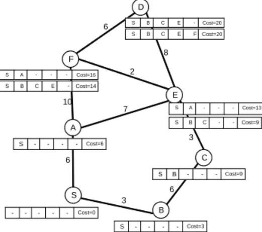
Therefore, we can calculate the route stability as the sum of additive costs. An illustrative example of using this scheme for ad-hoc routing is shown in Fig. 1 where the cost of each link is shown on it.

In route discovery phase of AODV, RREQ packet contains the addresses of source and destination nodes,

broadcast id, and hop count which will be updated by

each intermediate node. An additional field is required in order to put the cost of packet into RREQ message. Fig. 2 shows a brief view of the RREQ packet fields for the proposed scheme.

In order to implement DP approach in AODV protocol, in the route discovery phase of routing, the source node broadcasts RREQ packet with zero cost. When the first RREQ is received in relaying nodes, a table is created that we call RREQ table which is uniquely identified by source address and

broadcast id. Also, the cost field of the created entry is

updated by adding the link cost and RREQ cost field. For example, in Fig. 1 suppose F receives the first RREQ packet from A that its cost is 6. F adds the cost of AF link to packet cost and updates the cost field. If there is not any route entry toward source node in F, it creates a new entry which is used for the reverse route in RREP phase. Then a timer is started for a predefined duration that we call it 𝑡𝑑. If a RREQ with lower cost is received from other nodes before this timer is expired, the RREQ and route entry will be updated. Otherwise, the received RREQ packets are dropped. When the timer expired, the best RREQ with the lowest cost is rebroadcasted. Note that, increasing 𝑡𝑑, enhances the probability of finding more stable route. However, it imposes higher route discovery delay. In fact there is a tradeoff between the stable route discovery delay and the probability of loosing the most stable route. After receiving the first RREQ packet, destination node may wait the decision making with the hope of receiving better RREQ which leads to route discovery delay.

Following the route selection, the destination sends back the RREP message to fill the intermediate nodes S

B A

C E F

D

3 6

6 3 7

10 6

2 8

- - - Cost=0

S - - - - Cost=3

S B - - - Cost=9

S - - - - Cost=6

S A - - - Cost=13 S B C - - Cost=9 S A - - - Cost=16

S B C E - Cost=14

S B C E - Cost=20 S B C E F Cost=20

Source address

Destination address Source Sequence number Destination Sequence number

Broadcast id Cost

routing table and ignore the subsequent received RREQ messages.

The disadvantage of the above method is the route discovery delay. However, the overhead is comparable with the traditional AODV and in some cases is better than it. Also, our simulations results reveal that the overhead of our algorithm is very lower than the proposed algorithm in [11] in the case of the same scenarios.

V. ROUTE STABILITY AS A MINMAX PROBLEM In the previous section, the route stability measure is defined as the product of the links’ stability measures from which the route is traversing. Applying a log transformation makes the route stability measure to an additive function of the corresponding links’ stability measures. Then a DP algorithm is presented to find the stable route toward the destination. The drawback of this route stability measure is that the effect of less stable links may fade in these additive measures and is not reflected properly when there exists some strong stable links in the path.

In this section, we argue that the stable route selection can be better described as a MinMax problem. That is, the stability of a route, in essence, is determined by the least stable link on it. In other words, the stable route is the one for which the maximum link stability cost on it is minimized over the space of all available routes.

Let 𝑅𝑠 denotes the most stable route between 𝑆 and 𝐷. The problem is to find:

( 6 ) 𝑠 = 𝑎𝑟𝑔 max

𝑖=1,2,…,𝑀𝑡 𝑖 where 𝑡𝑖 _{is the lifetime of route 𝑅}

𝑖. As a MinMax problem, 𝑡𝑖 _{is given by:}

( 7 ) 𝑡𝑖_{= 𝑚𝑖𝑛 {𝑡}

𝑗𝑖, 𝑗 = 1,2, … , 𝑁𝑖}

Recall that 𝑡𝑗𝑖, and 𝑁𝑖 are the lifetime of 𝑙𝑛_𝑗𝑖,𝑛_𝑗+1𝑖 𝜖 𝐿𝑖 and the number of relay nodes on route 𝑖, respectively. Using (6) and (7) we have:

( 8 ) 𝑠 = 𝑎𝑟𝑔 max

𝑖=1,2,…,𝑀{𝑚𝑖𝑛 {𝑡𝑗 𝑖_{, 𝑗 =} 1,2, … , 𝑁𝑖}}

Let 𝜁 be a strictly decreasing function which convert the lifetime of each link to its cost, i.e., 𝐶𝑗𝑖= 𝜁(𝑡𝑗𝑖). Where 𝐶𝑗𝑖 is the cost of 𝑙𝑛_𝑗𝑖,𝑛_𝑗+1𝑖 . Using (2) we have:

( 9 ) 𝐶𝑖_{= 𝜁(𝑡}𝑖_{) = 𝑚𝑎𝑥 {𝜁(𝑡}

𝑗𝑖), 𝑗 = 1,2, … , 𝑁𝑖}

Where 𝐶𝑖 _{is the cost of 𝑅}

𝑖. Finally we have: ( 11 ) 𝐶𝑠_{= 𝜁(𝑡}𝑠_{) = 𝑚𝑖𝑛}

𝑖=1,2,…,𝑀{𝐶 𝑖_}

( 11 ) 𝑠 = 𝑎𝑟𝑔 min

𝑖=1,2,…,𝑀{𝑚𝑎𝑥 {𝐶𝑗 𝑖_{}, 𝑗 =} 1,2, … , 𝑁𝑖}

As (11) shows, the stable route selection problem cast as a MinMax problem. In the remainder of this paper we discuss how we can solve this problem in an

algorithmic manner that can be implemented in MANET’s routing protocols.

VI. A DP SOLUTION FOR MINMAX ROUTING

The routing procedure is a sequential decision making process when at the 𝑖𝑡ℎ _{stage each node selects} the next one. Let 𝑛𝑖(𝑗) denotes the 𝑖𝑡ℎ _{node in the 𝑗}𝑡ℎ stage of the routing procedure.

Consider the routes which are passing through 𝑛𝑘(𝑖 − 1). 𝐹𝑘(𝑖 − 1) and Γ𝑛𝑘(𝑖 − 1) denote the minimum lifetime of the links in the most stable route ending at (𝑖 − 1)𝑡ℎ _{stage and the node through which} this route is passed at (𝑖 − 2)𝑡ℎ _{stage, respectively.} We have the following proposition.

Proposition 1 If the most stable route through

𝑛_𝑘′(𝑖) is traversing 𝑛_𝑘(𝑖 − 1), then this route includes

the most stable route through 𝑛𝑘(𝑖 − 1), and 𝑙𝑛

𝑘′,𝑛𝑘.

Proof 1 By contradiction, assume that the most

stable route through 𝑛_𝑘′(𝑖), includes 𝑅_𝑔 and 𝑙_𝑛

𝑘′,𝑛𝑘, in

which 𝑅𝑔 is not the most stable route ending at 𝑛𝑘(𝑖 −

1). That is, 𝑡𝑔_{< 𝑡}𝑠_{, where 𝑡}𝑠 _{is the lifetime of the}

most stable route through 𝑛𝑘(𝑖 − 1). We have:

𝐹𝑘′(𝑖) = min {𝑡𝑔, 𝑇(𝑘, 𝑘′)}

Where 𝑇(𝑖, 𝑗) denotes the lifetime of 𝑙𝑛_𝑖,𝑛_𝑗. On the

other hand, 𝐹𝑘′(𝑖) should be the lifetime of the most

stable route through 𝑛_𝑘′(𝑖). Since:

min {𝑡𝑔_{, 𝑇(𝑘, 𝑘}′_{)} ≤ min {𝑡}𝑠_{, 𝑇(𝑘, 𝑘}′_)}

We find that the lifetime of the route which

includes the most stable route through 𝑛𝑘(𝑖 − 1) is

greater than 𝐹_𝑘′(𝑖) which is a contradiction.

Let us assume that the most stable route through 𝑛𝑘′(𝑖) is through 𝑛1(𝑖 − 1). According to Proposition

1, the most stable route’s lifetime at 𝑛𝑘′(𝑖) is given by

(12-13).

( 12 ) 𝐹𝑘′(𝑖) = min {𝐹1(𝑖 − 1), 𝑇(1, 𝑘′)}

( 13 ) Γ𝑛𝑘′(𝑖 − 1) = 𝑛1(𝑖 − 1)

As 12 ) indicates, the lifetime of the stable route ( ending at 𝑛_𝑘′(𝑖) is the minimum of the lifetime of the

previous stage of the route which passes through 𝑛1(𝑖 − 1) and the lifetime of the new link which is added to the route at 𝑖𝑡ℎ _stage.

Similarly, assume that the most stable route through 𝑛_𝑘𝑖′ is through 𝑛2(𝑖) . Then we have:

( 14 ) 𝐹_𝑘′(𝑖) = min {𝐹₂(𝑖 − 1), 𝑇(2, 𝑘′)}

( 15 ) Γ𝑛𝑘′(𝑖 − 1) = 𝑛2(𝑖 − 1)

In general, all nodes at stage 𝑖 − 1should be considered as the node through which the most stable route is passed and then goes through 𝑛𝑘′(𝑖).

( 16 ) 𝐹_𝑘′(𝑖) = 𝑚𝑎𝑥 {𝑚𝑖 𝑛{𝐹_𝑗(𝑖 −

1), 𝑇(𝑗, 𝑘′_{)} 𝑗 = 1,2, … , 𝑁}

( 17 ) Γ𝑛𝑘′(𝑖 − 1) = 𝑛_ℎ(𝑖 − 1)

Where

ℎ = 𝑎𝑟𝑔 max

𝑖=1,2,…,𝑁{𝜁(𝑖, 𝑗, 𝑘 ′_)} and

𝜁(𝑖, 𝑗, 𝛾) = min {𝐹𝛽(𝛼 − 1), 𝑇(𝛽, 𝛾)}

The problem is now broken down into sub problems of finding the most stable route ending at 𝑛𝑖(𝑗) 𝑖, 𝑗 = 1,2, … , 𝑁. The initialization step of this recursive procedure is given by (18) for 𝑖 = 1.

( 18 ) 𝐹𝑘′(1) = 𝑚𝑎𝑥 {𝑚𝑖 𝑛{∞, 𝑇(𝑆, 𝑘′)}

Which states that, without consideration of any loop in routing, the lifetime of a route which is started at 𝑆 and ended at 𝑆 is ∞. Therefore, the lifetime of the routes at stage 1 is given by:

( 19 ) 𝐹𝑘′(1) = 𝑇(𝑆, 𝑘′)

( 21 ) Γ𝑛𝑘′(1) = 𝑆

Finally, the recursive function is computed by: 𝐹𝑘′(𝑖)

= { 𝑇𝑆

𝑘′ _{𝑖 = 1 , 𝑘}′_{= 1,2, … , 𝑁} max {min{𝐹𝑗(𝑖 − 1), 𝑇(𝑗, 𝑘′)} 𝑖 = 2,3, . . , 𝑁

Γ_𝑛𝑘′(𝑖) =

{_𝑛 𝑆 𝑖 = 1

ℎ(𝑖 − 1) 𝑖 = 2,3, … , 𝑁, 𝑘′= 1,2, … , 𝑁

Note that, local information about the neighbors of each node is sufficient to deploy this recursive scheme.

Following computation of, 𝐹𝑘′(𝑖) and Γ𝑛𝑘′(𝑖), we can construct the most stable route between source and destination. Destination node may receive many RREQ packets with different number of hops. Assume 𝑓∗ _{and 𝛾}∗ _{denote the lifetime of the stable route} between 𝑆 and 𝐷 and the last node in this route before 𝐷.

( 21 ) 𝑓∗_{= max{𝐹}

𝐷(𝑖)} 𝑖 = 1,2, … , 𝑁

( 22 ) 𝛾∗_{= Γ𝐷( 𝑝 )}

Where

ℎ = 𝑎𝑟𝑔 max 𝑖=1,2,…,𝑁𝐹𝐷(𝑖)

If 𝐹𝐷(𝑖) = 0, it means that there is no route with 𝑘 hops between 𝑆 and 𝐷. Also, 𝑓∗_{= 0 means that there}

is no route between source and

destination. Algorithm. 1 summarizes the procedure to find the most stable route.

Using the above analysis, the AODV based implementation of MRA is available by changing the updating rule of the RREQ cost at each node in DP algorithm. It is sufficient to update the RREQ packet cost using the maximum of current RREQ packet cost and the cost of the link to the next adjacent node instead of adding these costs.

In Fig. 3, the RREQ packets are computed using MRA for the network topology in Fig. 1. It should be noted that the route discovery delay and route stability tradeoff is the same as it discussed in DP Algorithm.

VII. SIMULATION RESULTS

To assess the performance of the proposed algorithm, extensive simulations have been done using NS2-simulator [15]. We evaluate and compare the performance of the proposed scheme in terms of the route stability, delay and overhead for different scenarios. In these scenarios the density of nodes in the network and their mobility profiles are subject to change where the number of the nodes is varying from 20 to 60. In all cases, the nodes are uniformly distributed in 1400 × 300 𝑚2 _{area and the} transmission range of each node is assumed to be 250 meters. The mobility model of the nodes is Random Waypoint which their pause time is 5 seconds and the

Algorithm. 1 MinMax based Ad hoc routing algorithm //Initialization Phase:

Computes 𝜁(𝑇(𝑘, 𝑘′_{)), ∀ 𝑘 𝜖neighbors of 𝑘}′ _{using (2).}

The source broadcasts RREQ (srcaddr;desaddr;srcseq number;desseq number;brid;cost).

//Broadcasting Phase or Route Discovery Phase: for each node that receives RREQ do

if (𝑘′ _{== src addr) then}

drop RREQ else

create a RREQ table (src;bid;rreqcost) src← src addr

bid ← br id

rreqcost ← 𝑚𝑎𝑥( 𝑐𝑜𝑠𝑡, 𝜁(𝑇(𝑘, 𝑘′₎₎₎

Γ𝑛_𝑘′(𝑖) ← 𝑘

start a timer with td duration wait to get more identical RREQ for new arrived RREQ during 𝑡𝑑 do

if (cost < 𝜁(𝑇(𝑘, 𝑘′_{))) then}

cost ← 𝜁(𝑇(𝑘, 𝑘′₎₎

end if

if (rreqcost > cost) then rreqcost ←cost Γ𝑛_𝑘′(𝑖) ← 𝑘

end if

if the timer is expired then if (𝑘′ _{!= des addr) then}

rebroadcast the best RREQ else if (𝑘′ _{== des addr) then}

send back the RREP packet through Γ𝑛_𝑘′(𝑖)

end if end if end for end if end for

Fig. 3 MRA route discovery phase for routing. maximum velocity, 𝑉𝑚𝑎𝑥, is changing from 5 𝑚/𝑠 to 40 𝑚/𝑠. Also, IEEE 802.11 is set as the MAC layer protocol and nodes use RTS/CTS based DCF to transmit their packets. Queue buffer lengths of all nodes are the same that is assumed 50 packets. When buffers are overflow, the DropTail mechanism is deployed for packet dropping. Moreover, all nodes use omni-directional antenna. The reported results are the average and confidence interval (95%) of performance parameters for 100 times simulation runs where each simulation last for 500 seconds. Simulation parameters that are used in our work are summarized in Table. 1. Packets use UDP as their transport layer protocol and Constant Bit Rate (CBR) is used as their packet arrival model. The size of packets in all simulations is 500 bytes and their arrival rate is 240 Kbps.

A. Stability of Selected Routes

The CDF of routes’ lifetimes of the three algorithms are shown in Fig. 4. In this simulation we consider a MANET consists of 𝑁 = 5and 𝑉𝑚𝑎𝑥= 15 𝑚/𝑠 . Hello interval in the MRA and AODVS1 [11] are assumed 10 seconds and 1 seconds respectively. This figure shows that the probability of route breaking before a given time for MRA is less than two other algorithms which means MRA finds more stable routes compared to two other schemes. As the graph reveals, the probability that a selected route disconnects before 40 seconds in MRA is about 0.33. This probability for AODV and AODVS1 [11] is about 0.47 and 0.46 respectively. Note that, in AODVS1, if the Hello interval increases, the result will be worse than the reported graph in Fig. 4. As mentioned earlier, the reason is that in AODVS1 the stability measure is depend on Hello packets interval and the measurement become more accurate as the this interval decreases.

Table. 1 Simulations parameters Number of nodes 20N60

Network area 1400 × 300 𝑚2

MAC protocol IEEE 802.11 Maximum Node

speed

5𝑚/𝑠 < 𝑉𝑚𝑎𝑥< 40 𝑚/𝑠

Drop policy DropTail

Antenna type Omni-Directional

Basic rate 2 Mbps

Slot time 50 s

DIFS time 128 s

SIFS time 28 s

Propagation delay 1 s

Fig. 4 The CDF of average route life time for AODV, AODVS1[11] and MRA, 𝑁 = 50, 𝑉𝑚𝑎𝑥=

15 𝑚/𝑠, Hello interval = 10 Seconds.

In the next simulation the mobility profile of nodes is changed and lifetime of the selected route by each algorithm is evaluated. 0 shows the mean lifetime of the selected routes for different maximum nodes’ velocities.

The simulations have been done for 𝑁 = 20and 𝑁 = 60. As expected, the lifetime of the selected route of all schemes is decreased as the nodes’ velocity is increased. From this graph we can find that in all cases the MRA algorithm has better performance and the average lift time is longer than the other algorithms, specially, when 𝑉𝑚𝑎𝑥 is lower than 15 𝑚/𝑠. It should be noted that the average life time in the dense network is higher than the sparse one. The reason is that in dense networks the probability of existing more routes between source and destination is increased compared to sparse networks. However, in both cases, when 𝑉𝑚𝑎𝑥 is increased, the CDF of average routes life time becomes similar.

B. Total Overhead

In Fig. 6, the total overhead of three investigated schemes for different number of nodes, 𝑁, is compared. Also, in this figure the total overhead for two maximum velocities, 𝑉𝑚𝑎𝑥= 5 𝑚/𝑠 and 𝑉𝑚𝑎𝑥= 40 𝑚/𝑠 , is

depicted. As the figure shows, AODVS1[11] has the maximum overhead and as 𝑁 increases the overhead of this scheme is increased remarkably. Whereas, in MRA and AODV the trend is fairly flat. It means that increasing N has minor effect on total overhead of AODV and the proposed scheme. Comparison of MRA and AODV in the case of 𝑉𝑚𝑎𝑥= 40 𝑚/𝑠 reveals that

except for 𝑁 = 20, the total overhead of MRA when 𝑁 is varying from 30 to 60, is lower than AODV indicating

better performance of MRA.

Fig. 5 Comparison of the route’s average lifetime for shortest path AODV, AODVS1 [11] and MRA for different maximum speed of nodes, 𝑁 = 20, 𝑁 = 60. S

B A

C E F

D

3 6

6 3 7

10 6

2 8

- - - Cost=0

S - - - - Cost=3

S B - - - Cost=6

S - - - - Cost=6

S A - - - Cost=7 S B C - - Cost=6 S A - - - Cost=10

S B C E - Cost=6

S B C E - Cost=8 S B C E F Cost=6

Fig. 6 Total overhead vs. number of nodes for AODV, AODVS1 [11] and MRA,𝑉𝑚𝑎𝑥=

5 𝑎𝑛𝑑 40 𝑚/𝑠.

We also consider the effect of 𝑉𝑚𝑎𝑥 on the total overhead for𝑁 = 60. As Fig. 7 illustrates, the overhead of three schemes is proliferated as 𝑉𝑚𝑎𝑥 is

increased. However, the increasing rate of total overhead in AODVS1 [11] is greater than the AODV and MRA. Moreover, the overhead in AODVS1 is three times greater than the other methods. Also, closely looking at the figure shows that when 𝑉𝑚𝑎𝑥 is

changing from 10 𝑚/𝑠 to 40 𝑚/𝑠, overhead of MRA is lower than AODV which shows that as the nodes mobility is increased, MRA requires less cost in order to find more robust routes.

C. Route Discovery Delay

As discussed earlier, there is a tradeoff between route discovery delay and the chance of finding better routes by receiving more RREQ packets. To demonstrate the effect of route discovery waiting time on routes life time, 𝑡𝑑 is changing from 1𝑚𝑠 to 30 𝑚𝑠. Fig. 8 shows the CDF of route life time in a network with 𝑁 = 50 and 𝑉𝑚𝑎𝑥= 15 𝑚/𝑠. As the graph represents, in the case of 𝑡𝑑= 1𝑚𝑠 the MRA results is fairly comparable with AODV and for 𝑇𝑖𝑚𝑒 > 80seconds is worse than AODV. As 𝑡𝑑 increases, the CDF of route life time is improved and for 𝑡𝑑= 20 𝑚𝑠 the best performance is achieved. It has been mentioned that as 𝑡𝑑 is increased, the probability of receiving better RREQ rising, which lead to increase the life time. It should be noted that increasing 𝑡𝑑 is related to have more delay in route discovery phase. Consequently, there is a tradeoff between finding a long life route and route discovery delay.

Fig. 7 Total overhead vs. maximum speed of nodes for AODV, AODVS1 [11] and MRA,

𝑁 = 60.

Fig. 8 CDF of the average routes life times which are selected by MRA for different route discovery delay, 𝑁 = 50 , 𝑉𝑚𝑎𝑥= 15 𝑚/𝑠

VIII. CONCLUSION

The stable route selection in wireless ad-hoc networks is formulated as a MinMax problem and a dynamic programming based algorithm is proposed to solve it. The proposed scheme can find the most stable route in the network and can be implemented in existent routing protocols like AODV provided that each node has an estimate of its neighbors mobility profile. Also, discussing the tradeoff between the route discovery delay and its stability, it is shown that in the proposed scheme this delay is comparable to the shortest path AODV scheme and is independent of network parameters. Extending the results for other mobility models and finding the optimum 𝑡𝑑 to have less overhead and discovery delay is the topic of future work.

REFERENCES

[1] J. Corson, S., Macker, “Mobile ad hoc networking (MANET): Routing protocol performance issues and evaluation considerations.,” Mob. Ad-hoc Netw. Work. Gr., 2003.

[2] J. Schiller, Mobile communications. Addison Wesley, 2003.

[3] C. E. Perkins and E. M. Royer, “Ad-hoc On-Demand Distance Vector Routing.,” in Proceedings of the Second IEEE Workshop on Mobile Computer Systems and Applications, 1999, pp. 90–100.

[4] B. An and S. Papavassiliou, “An entropy-based model for supporting and evaluating route stability in mobile ad hoc wireless networks,” IEEE Commun Lett., vol. 6, pp. 328– 30, 2002.

[5] G. Carofiglio, C. F. Chiasserini, M. Garetto, and E. Leonardi, “Route Stability in MANETs under the Random Direction Mobility Model.,” IEEE Trans Mob. Comput, vol. 8, pp. 1167–79, 2009.

[6] M. Al-Akaidi and M. Alchaita, “Link stability and mobility in ad hoc wireless networks.,” IET Commun, vol. 1, pp. 173–78, 2007.

[7] X. M. Zhang, F. F. Zou, E. B. Wang, and D. K. Sung, “Exploring the Dynamic Nature of Mobile Nodes for Predicting Route Lifetime in Mobile Ad Hoc Networks,” IEEE Trans Veh Technol, vol. 59, pp. 1567–72, 2010. [8] A. B. McDonald and T. F. Zanti, “A mobility-Based

Framework for adaptive Clustrering in Wireless Ad Hoc Networks.,” IEEE J Sel. Areas Commun, vol. 17, pp. 1466–87, 1999.

[9] H. Zhang and Y. N. Dong, “A Novel Path Stability Computation Model for Wireless Ad Hoc Networks.,” IEEE Signal Process. Lett., vol. 41, pp. 928–31, 2007. [10] J. Tang, G. Xue, and W. Zhang, “Reliable Ad Hoc

Routing Based On Mobility Prediction.,” J Comb Optim., vol. 11, pp. 71–85, 2006.

[11] N. Chama, R. C. Sofia, and S. Sargento, “Multihop Mobility Metrics based on Link Stability.,” in In 27th Internatinal Conference on Advanced Information Networking and Applications Workshops, 2013, pp. 809– 16.

[12] K. Mahajan, M. A. Rizvi, and D. Singh Karaulia, “path optimization of aodv by eo-aodv in manet,” in ICTCS ’14 Proceedings of the 2014 International Conference on Information and Communication Technology for Competitive Strategies, 2014.

[13] T. Camp, J. Boleng, and D. V., “A Survey of Mobility Models for Ad Hoc Network Research.,” Wirel. Commun. Mob. Comput., vol. 2, pp. 483–502, 2002. [14] W. Su and M. Gerla, “IPv6 Flow Handoff in Adhoc

Wireless Networks Using Mobility Prediction.,” in Proceedings of IEEE Global Telecommunication Conference, 1999, pp. 271–5.

[15] “Network Simulator---{NS} (Version 2).” [Online]. Available: http://www.isi.edu/nsnam/ns/.

[16] D. P. Bertsekas, Dynamic Programming and Optimal Control. Athena Scientific, 2000.

Abdorasoul Ghasemi received his B.Sc. degree (with honors) from Isfahan University of Technology, Isfahan, Iran and his M.Sc. and Ph.D. degrees from Amirkabir University of Technology (Tehran Polytechnique), Tehran, Iran all in Electrical Engineering in 2001, 2003, and 2008, respectively. He is currently an Assistant Professor with the Faculty of Computer Engineering of K. N. Toosi University of Technology, Tehran, Iran. His research interests include communication networks, network protocols, resource management in wireless networks, and applications of optimization and game theories in networking.

Mahmood Mollaei received the B.Sc. degree in Electrical Engineering from Tabriz University, Tabriz, Iran, in 2004 and the M.Sc. and Ph.D. degree both in Electrical Engineering from K. N. Toosi University of Technology, Tehran, in 2008 and 2014, respectively. His current research interests include performance analysis of wireless networks, network management, and quality of service.