1118.pdf

ABSTRACT

ACKNOWLEDGEMENTS

This research was made possible by a grant from the Water Resources Research In¬ stitute.

I would like to thank Dr. Cass T. Miller for his patience, guidance, and assistance, and especially for providing me with the opportunity to do this work. Also, thanks to my committee for their involvement, and to my fellow students, whose encouragement and

TABLE OF CONTENTS

Page

Abstract... i

Acknowledgements... ii

Table of Contents... iii

List of Figures... v

List of Tables ... vii

1. Introduction ... 1-1

2. Theoretical Background... 2-1 2.1 Darcy's Law... 2-1 2.2 Partially-Saturated Flow... 2-3 2.3 Fltiid-Phase ADR Equation ... 2-7

2.3.1 Velocity Vector... 2-8

2.3.2 Hydrodynamic Dispersion... 2-8 2.4 Vapor-Phase ADR Equation... 2-10

2.5 Diffusion... 2-11

2.5.1 Steady State... 2-11

2.5.2 Transient... 2-12

2.6 Reactions ... 2-14

2.6.1 Aqueous-Solid Equilibrium... 2-14

2.6.2 Aqueous-Solid Rate... 2-16 2.6.3 Vapor-Liqmd Equilibrium ... 2-18 2.7 Governing Equations ... 2-20 3. Experimental Methods... 3-1

3.1 Introduction... 3-1 3.2 Materials ... 3-3

3.3 Analytical Methods... 3-6

3.3.1 Extraction Methods... 3-6 3.3.2 Measurement Methods... 3-7

3.4 Experimental Methods... 3-9 3.4.1 Field Sampling... 3-9

3.4.2 Bottle-Point Isotherm... 3-9

3.4.3 Bottle-Point Rate Study... 3-11 3.4.4 Diffusion Coltmm Experiments ... 3-13 3.4.4.1 Description of Apparatus... 3-13 3.4.4.2 Column Preparation... 3-15 3.4.4.3 Sampling Procedure... 3-15

Page

4. Experiment2d Results... 4-1

4.1 Field Results... 4-1

4.2 Sorption Study Results ... 4-5

4.3 Diffusion Column Results ... 4-11

4.4 Modeling Results... 4-11

5. Discussion... 5-1 5.1 Diffusivity... 5-1 5.2 Sorption... 5-5

5.3 Impa,ct at the Field Scale ... 5-19

LIST OF FIGURES

Page 1-1 Groxmdwater Subsurface Zones... 1-2

1-2 NAPL in the Vadose Zone... 1-4:

1-3 Partitioning in the Subsurface... 1-5

3-1 Grain Size Distribution of Pope AFB Soil... 3-5 3-2 Aqueous Extraction Procedure... 3-8 3-3 Field Sampling Procedure... 3-10 3-4 Procedure for Bottle-Point Studies... 3-12 3-5 Diffusion Apparatus ... 3-14 4-1 Topographic Map of Fire Training Area No. 4... 4-2 4-2 Groundwater Elevations at Fire Training Area No. 4... 4-3 4-3 Normalized Concentrations of Hydrocarbons in the Partially-Saturated Zone 4-4 4-4 Results of Bottle-Point EquiUbrium Study... 4-6 4-5 FreundHch and Linear Isotherm Models... 4-7 4-6 Rate Study Results: Time vs. Concentrations ... 4-9

4-7 Rate Study Results: Time vs. C/Co ... 4-10

4-8 Results of Column B-1... 4-12 4-9 Results of Coliman C-1... 4-13 4-10 Results of Colimm B-2... 4-14 4-11 Results of Column B-3... 4-15 4-12 Results of Column C-3... 4-16

4-13 Results of Column B-4... 4-17

4-14 Comparison of Model: Kp = 0 ... 4-20 4-15 Comparison of Model: isTp = 0.37... ... . . . 4-21

4-16 Comparison of Model: Kp = Best Fit ... 4-22

5-1 Comparison of Tortuosities ... 5-4

5-2 Simulation of .Colvmrn B-1: Kp = 0...^^^:-<^7 T''^. ... 5-8

Page

5-4 Simulation of Coliman B-2: Kp = 0... 5-10

5-5 Simulation of Column B-3: iifp = 0... 5-11 5-6 Simulation of Coltunn C-3: Kp = 0... 5-12 5-7 Simulation of Column B-4: Kp = 0... 5-13 5-8 Simulation of Column B-1: Best Fit iiT,... 5-14

5-9 Simulation of Column C-1: Best Fit iiTp... 5-15

LIST OF TABLES

Page

3-1 Physical and Chemical Properties of Toluene... 3-4

4-1 Sximmaxy of Experimental Equilibrium Parameters... 4-8 4-2 Summary of Diffusion Column Data ... 4-18

5-1 Published Tortuosity Factors and Variance with Experimental Data .... 5-3

>^^

1 INTRODUCTION

In the United States, grotmdwater has become one of our most essential and most

exploited natural resources. We depend on groundwater for industrial and domestic use

for a number of reasons. In some areas, such as the southwest, large influxes of people have raised the demand for water in a region where surface water is not abtindant. In other areas

of the country groundwater is preferred to surface water because it is a more reliable water

source. Annual and seasonal fluctuations are much more pronounced in surface water, and surface water may not be convenient because it occurs at specific points, at springs, lakes or rivers. Dependence on groundwater has also required less long-range planning because there has always been a seemingly endless supply of it; as the population of a region grows we simply install axiother well. Another advantage of groundwater has been its superior quality; surface water is generally more susceptible to man-made waste, either by run-off

or by direct dumping.

Groundwater supplies, however, are neither infinite nor indestructible. Aquifers are fragile, delicately-balanced natural systems which, because of their dynamic nature, are easily contaminated, and difficult to restore. Recharge to an aqviifer system occurs mainly through contact with surface water and by infiltration of rain water. This recharge water filters through the subsurface environment, which can be divided into four general regions: the soil zone, where plant life is supported; the vadose, or partially- saturated zone; the saturated zone; and the capillary fringe zone, which is the interface between the saturated and unsaturated zones. Figvire 1-1 is a diagram of groimdwater subsurface zones.

Groundwater contamination may occur in various ways. Contaminants in surface

water or spilled or dimiped on the groimd svirface in a recharge zone may be carried

through the soil zone and into the vadose and satvirated zones by the natural recharge

GROUND SURFACE

UNSATURATED ZONE

RATED ZONE

WATER TABLE

IMPERMEABLE LAYER

• )

m^mmmsmmmmt

storage tanks (USTs), which are used to store gasoline and industrial chemicals. The

Ufetime of most existing tanks is approximately 18 years, and it was estimated that as

many as 100,000 tanks were leaking in the U.S. in 1985 (Mackay et al., 1985).

Contaminants that have a higher density than water that pass through the vadose

zone and into the saturated zone may pass through this region and eventually acc\unulate

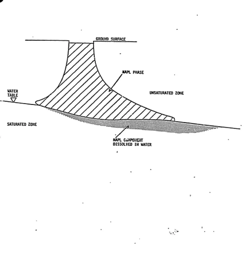
at the bottom of the aquifer. However, organic compovmds that are less dense than water,

such as many components of gasoline, will remain at the top of the saturated zone and gradually go into solution in the groimdwater. Some contaminants will remain as residuals

in the vadose zone as well, as is shown in Figure 1-2. In the saturated zone a contaminant

may sorb onto the soil from the Uquid phase, and once on the solid it may desorb back

into the grovmdwater. The contaminant may be transported by the bulk movement of

the groimdwater and it may disperse through the groundwater by molecular movement and mechanical mixing. Many large hydrocarbons will, in time, chemically degrade into smaller chemical species. Biological degradation also accounts for the destruction of many

groundwater contanainants.

Contaminants that remain in the partially-saturated zone may partition into the vapor phase as well as sorb onto solids (Figure 1-3). Movement of contaminants in this region

can occur by btdk movement of the vapor phase or by vapor-phase diffusion. Both chemical and biological degradation may also occur in this region.

Traditionally, the evaluation of a contamination problem has been based on measure¬

ments from the saturated zone. Measurements of the free product, that is the contaminant

floating on the groundwater, and of the location of the contaminant plume have been used

to determine the extent of a spill and also to identify the source of a contaminant. Relying

on meastirements from the saturated zone are not always adequate for these evaluations.

For the cases where the contamination includes low-density hydrocarbons, a large volume

of these compounds may reside in the vadose zone. In this region the movement of the

GROUND SURFACE

WPX. PHASE

WATER

TABLE

UNSATURATED ZONE

SATURATED ZONE

HAJn. CiW4P0;JEIU

DISSaVED IH WATER

Figure 1-2. Non-Aqueous-Phase Liquid in the Vadose Zone.

#

WATER

m

difFxise from axeas of high concentration to areas of low concentration, volatile organic com¬ pounds may migrate in any direction away from a source, including up-gradient from that source. Once away from the area of high concentration the volatile organic compounds (VOCs) will establish a new vapor-liquid equilibrivun and some will eventually end up in

the groundwater even up-gradient from the soiurce.

The partially- saturated zone can hold great volumes of VOC vapor, and migration of

these vapors by diffusion, although slow, may occur over large distances. The result is that,

over time, the source of a contaminant spreads; what was once a small point source may

become a large source area. Diffusion of VOCs not only creates a problem in identifying

the source of a contaminant, it also complicates restoration of a contaminated aquifer. The cleanup of contaminants in the subsurface may be a small-scale operation if the remedial

action is talcen immediately after the release. But the longer the VOCs are left to diffuse

through the partially-saturated zone, the larger the source area becomes, and thus, the

larger the area requiring remedial action. Restoration of the saturated zone must therefore

be coupled with restoration of the vadose zone which, with time, may become a significant sovirce of additional contamination.

Steady-state diffusion through porous media has been studied by some researchers in

order to determine the rate of movement of pesticides, herbicides, or nutrients through

the soil (van Genuchten et al., 1977; Albertson, 1979). Researchers have also attempted to quantify the rate at which benzene or other industrial waste products vaporize out of landfills (Farmer et al., 1980; Karimi et al., 1987), and others have determined the diffusion parameters at potential hazardous waste disposal sites to determine how effectively the waste will be contained (Weeks, 1982). The characteristics of transient diffusion in porous media have only recently begun to receive attention due to the large niimber of sites at

with these sites, which was discussed earher. The objective of this work was to quantify the

transient nature of vapor-phase diffusion in the partially- saturated zone, while accounting

2 THEORETICAL BACKGROUND

2.1 Darcy's Law

In the year 1856 a French engineer named Henry Darcy developed an empirical law

that governs the flow of water through porous media. Darcy's experimental apparatus

consisted of a satvirated cylinder of porous media. Water flowed in one end of the cylinder

at flow rate Q, and flowed out the other end at the same flow rate. Each end of the cylinder

was connected to a reservoir suspended above it, each at a different height, hi and /12. The experiments consisted of varying hi, /12, and Al, the length of the column, and measuring

the resiilting flow rate out of the column. The specific discharge, qx is defined as:

Q

9x = 5 (2-1)

where A is the cross-sectional area of the coltmin and q^ has units of length per time.

Darcy fotmd that the specific discharge is directly proportional to the difference in reservoir

elevations, hi — /12, for constant A/, and inversely proportional to A/ for constant Ah:

Ah

9- = -^^ (2-2)

or

dh

i. = -K^ (2-3)

The hydraulic conductivity was examined more careftdly by Hubbert in 1940. Hubbert

was looking for a way to separate the effect of the flmd properties from the media properties

in the hydraulic conductivity. He deflned the hydrauHc conductivity as:

K=^-^ (2-4)

where p is the density of the fluid; /x is the dynamic viscosity of the fluid; g is the grav¬

2.2 Partially-Saturated Flow

The governing equation for the flow of fluid in the partially-saturated zone can be

derived using a control-volume approach. A mass balance on a control volume of partially-saturated media may be written:

MassAccumulated = Massin — MassOut (2-5)

which can be represented mathematically by:

^=Mir.-Moui (2-6)

where M is the mass of fluid. Describing the mass of fluid passing through the volvune in

one direction, x, in terms of the variables of the system, we have:

ͣ

^(pwVnS) = Ap^qin - \Apr„qin +

ͣ

^(Aprt,qx)/^xj (2-7)

where /9u, is the density of water; V is the volume of the control element; n is the porosity of the media; S is the degree of water saturation; A is the area of the face of the control volume normal to the x direction; and qx is the x component of the specific discharge

vector. This equation simplifies to:

-^{prvVnS) = -—{Ap^q^)Ax (2-8)

Adding the contributions to the control voltraie from the y and z directions, including the condition that the control volvune is constant, and introducing the relationship:

where 9y, is the volumetric fraction of the water phase, we get:

Q O O «3

This equation can also be written:

V-(/=>u,9-)=-^Mu,) (2-11)

To define the specific discharge vector, q, we start with the general form of Daxcy's law:

d<f> d<f> d(j)

^^ = ~^y'Ii~^^^^-^''Tz ^^"^^^

where Kxx-, Kxy, etc. are elements of the hydraulic conductivity tensor, and (j> is the

hydraiilic head defined as:

<^ = 0+ —= z + V' (2-15) P9

If the control volume is aligned with the principal axes we can drop the non- diagonal

terms of the hydrauHc conductivity tensor. Now, substituting Darcy's law into our working

equation gives:

d_

If changes in fluid density are assumed to be smeill compared to changes in moisture

content the equation becomes:

d

d.

K-O-l(-'<0-IHS-^ ^-"'

A more common form of the flow equation for partially saturated media is Richard's

equation. In Richard's equation the dependent variable is pressure head, ij), rather than

having two dependent variables, xj) and ^u,, as in equation 2-17. The use of pressiure head

as the dependent variable is generally preferred because of the dimensional convenience

(Parker et al, 1987). Making this conversion gives:

(2-18)

The specific moistvire capacity, c(^), is defined as the slope of the volmnetric moisture

content as a function of the pressure head:

c(« = ^ (2-19)

Making this final substitution gives Richard's equation:

d_

dx

HS+IHS)+IHf+^')-wf (2-^0)

The most significant simplifying assumption in Richard's equation is that the pressure in

the vapor phase is atmospheric (Faust, 1985).

In this development of Richard's equation both the hydraulic conductivity, K, and

functions have been found to be nonlinear and hysteretic in nature (Kool and Parker, 1987;

Kool and Parker, 1988). These relationships are important because they determine the

relationship between aqueous flow zuid saturation in the partially-saturated zone. This

means that changes in pressure head, hence satiu:ation,has a significant impact oh the

2.3 Fluid-Phase Advective-Dispersive-Reactive Equation

The advective-dispersive-reactive (ADR) equation is generally used as the macroscopic

equation that governs the fate and transport of groimdwater contaminants, though some

researchers have proposed other approaches (GiUham et al., 1984; Tompson, 1986). There

axe several ways to develop the ADR equation, including the use of the control volume

approach, as was used in the development of the flow equation. The derivation of the

transport equation will not be presented here, however. The general form of the ADR

equation is:

dCg

dt

= -V- grad C„ + div (Dfc grad Co) + V{Ca) + {j^\ (2-21)

where Ca is the aqueous concentration of contaminant; v is the vector of average

ground-water pore velocity; D^ is the hydrodynamic dispersion tensor that includes the effects

of both mechanical dispersion and molecular diffusion (Bear, 1979); and V{Ca) represents

either a mass source or sink within the control volume. The reaction term accounts for

any mass that is abided or removed by reaction. This term includes biological degradation,

chemical transformations, sorption onto the soUd phase, and desorption from the solid

phase.

In the partially-saturated zone contaminant transport may occin: in two phases, fluid

and vapor, and therefore the ADR equation must be formulated and solved for eax;h phase.

For the fluid phase, ignoring any internal sources or sinks, the ADR equation can be

written:

Velocity Vector

The pore velocity vector, v, describes the average linear macroscopic velocity of the

fluid phase zind is obtained by solving Richard's equation for partiaUy-satmrated flow. The

pore velocity is related to the specific discharge, q, by the relationship:

v = f (2-23)

where 0^) is the fluid-filled porosity of the media. The specific discharge defines a lin¬

ear velocity through a control volimie of media. The pore velocity refers to the average

ma<:roscopic pore velocity of the fluid.

Hydrodynamic Dispersion

Bear (1979) describes the hydrodynamic dispersion tensor as the sxim of a mechanical

dispersion term and a molecular diffusion term:

Dij=aTvSij+{aL-ocT)viVj/v + Dm (2-24)

where D,j is the i j term of the dispersion tensor; oct is the transverse dispersivity; ai is

the longitudinal dispersivity; v is the average magnitude of the groundwater velocity; 6ij

is the Kronecker delta function (6 = 1 {or i = j; 6 = 0 for i ^ j); and Dm is the effective

molecular diffusion coefficient.

Mathematical solutions to the ADR equation have been proposed and have compared

well with the results of laboratory experiments. However, discrepancies occvir between the

results of laboratory experiments and field experiments. Some researchers have concluded

that the discrepancies occur because dispersivity is a scale-dependent paxameter (Sudicky

amd Cherry, 1979; Pickens and Grisak, 1981). The dispersivity may be scale-dependent

The product of the flow velocity and the dispersivity is generally known as the me¬

chanical dispersivity. In groundwater systems the molectdar diffusion term. Dm, is often

very small relative to the mechanical dispersion, and may be neglected if groundwater

velocities axe large. One should note that the grovindwater velocity is present here in the

2.4 Vapor-Phase Advective-Dispersive-Reactive Equation

In the partially-saturated zone the advective-dispersive-reactive equation caji be writ¬

ten to describe contaminant transport in the vapor phase. Assuming that there are no

internal sources or sinks the equation is:

^ = -v . grad C„ -f- div (Dfc grad C„) + (^^ (2-25)

It is common, though possibly rash, to assmne that the pore velocity in the vapor

phase is negUgible and therefore that the effect of mechanical dispersion is small compared

to that of molecular diffusion (van Genuchten and Wieranga, 1976; Weeks et al, 1982;

Peterson et al, 1988). If one asstunes that the velocity approaches zero the ADR equation

reduces to:

^ = div(D.gradC„)+(^) (2-26)

Also as the velocity approaches zero, the hydrodynamic dispersion tensor can be

rewritten. Assuming that the effective diffusivity is the same in all directions, that there

axe no variations in media properties that could lead to anisotropic diffusion, the governing

equation becomes:

2.5 Diffusion

Steady-State Diffusion

Steady-state diffusion of a vapor through air was first described by Fick when he drew

an analogy between molecular difFiision and heat transfer in solids. Fick recognized that

the amount of vapor diffusing along a path length x is proportional to the concentration

gradient a<:ross this distance. Just as the conductivity, K, is the constant of proportionality

for heat transfer, Fick defined the diffusivity, £)*, as the constant of proportionality for

diffusion (Bird et al, 1960). Thiis Fick's First Law can be written:

j = _D*^ (2-28)

where, J is the flux; D* is the diffusion coefficient for the diffusion of one pure gas through

another; and dCy/dx is the concentration gradient.

In the case where a vapor is diffusing through porous media there axe several ap¬

proaches that may be taken to describe diffusion. One approach is to define an effective

diffusivity in which case Fick's first law is written as in equation 2-28. In this case the

effective diffusivity is a value that is specific to the media and to the conditions under

which the diffusivity was determined. These conditions include temperature, bulk density,

water content, and presence of other solutes.

A common way of describing diffusion in porous media is to define a tortuosity factor,

which accounts for the geometric effects of the solid media on the apparent diffusion. This

tortuosity factor accounts for the increased path length of diffusion and therefore includes

effects of water content. The steady-state diffusion equation for porous media can therefore

ͣ

fP^HWww^—^m

J = -dorD* ^ = -eoD, ^ (2-29)

where dj^ is the drained porosity of the soil, or the fraction of the total volume that is

occupied by air; r is the tortuosity, and D^ is an effective diffusivity. Empirical equations

for the tortuosity factor have been determined by various researchers (Buckingham, 1904;

MiUington, 1959; Millington and Qmrk, 1961; Albertson, 1979). The most commonly

accepted equation has been that proposed by MiUington and Quirk (1961). However,

even Millington and Qmrk's tortuosity has been found to be inaccurate by some recent

researchers (Peterson et al., 1988).

Transient Diffusion

The ADR equation for vapor-phase contaminant transport, neglecting velocity effects,

sorption effects and chemical reactions reduces to:

dt = D*V^C„ (2-30)

This equation is also known as Fick's second law of diffusion (Bird et al, 1960). Fick's

second law is applicable to the movement of one gas through another with no net flow of

gas (convection) and under isothermal, constant density conditions. Fick's second law was

also originally derived by analogy to heat transfer, and therefore many solutions to the

transient diffusion equation under a variety of boundary conditions are available in the

literature (Carslaw and Jaeger, 1959; Crank,1975)

Fick's second law can be adapted to describe diffusion in porous media:

This equation also assumes that molecular diffusion is the only means of vapor transport,

2.6 Reactions

Reactions between volatile organic chemicals (VOCs) and the soUd matrix retard the

movement of the chemical through that matrix. In the partially- satxirated zone, in the

absence of advective transport in the vapor phase, vapor-phase diffusion may be the most

significant method of transport of VOCs, but there are other physical phenomena that

play an important role. By definition the partially-saturated zone retains some residual

saturation, which creates a complex and tortuous path through which an organic vapor

must move. Throughout this partially-saturated zone the vapor is in contact with water as well as air and partitioning of the organic solute occurs between the aqueous and vapor

phases. Because the residual water is in contact with the solid phase, partitioning occurs

in turn between the axjueous and solid phases. The result is a dynamic system consisting

of three phases.

Aqueous-Solid Equilibrium

Sorption and desorption refer to the processes of transfer of mass from the fluid phase

to the soUd phase and from the solid phase to the fluid phase, respectively. The transfer

of an organic compound between a fluid and a solid phase is generally believed to be

a partitioning phenomena, and this partitioning has been found to be a function of the

fraction of organic matter present in the soil (Karickhoff, 1979). When the rate of transfer

of mass from the fluid phase to the solid phase is equal to the rate of transfer in the

opposite direction, the system is in a state of dynamic equilibrium.

Several models have been used to describe sorption equilibrium. The most common

of these is the Unear equilibrium model:

qe = KpCae (2-32)

of solid; Cac is the equilibritun fluid-phase concentration with units of mass per volume;

and Kp is the linear eqmlibriiun partitioning coefficient with units of volume per mass.

There are many empirical expressions for the partitioning coefficient. One such expression

for the partitioning of organic compomids in sediments has been described as (Karickhoff,

1979):

ͣ

^p = foc^oc (2-33)

where foe is the fraction of organic carbon in the soUd; and Koc is the organic-caxbon

partition coefficient of the soUd. Karickhoff found the organic-carbon partition coefficient

to follow the empirical expression:

log Koc = log i^ou, - 0.21 (2-34)

where Kow is the octanol-water partition coefficient of the solute. Octanol-water coeffi¬

cients axe compiled in the literature for a variety of compounds (Hansch and Leo, 1979).

This relationship was derived for soils of relatively high organic content, and may not

yield accurate predictions of Kp in soils of low organic carbon content (less than 0.1 per¬

cent). Also, the expression was derived for use with neutral, non-polar, and hydrophobic

compotmds and will not give accurate results if used for other types of compounds.

There axe also nonlinear equilibrium models. The most common of these is the

Fre-undUch sorption equilibrium model:

?e = KfC^I (2-35)

models this behavior more accurately than a lineax model. The great advantage of the

linear model, of course, is its simplicity.

Aqueous-Solid Rate

In a system for which the rates of sorption and desorption have not reached an eqtiilib-rium, it is necessary to determine the rate of sorption in order to thoroughly characterize the mass-transfer process. There axe several models that are used to describe the rate of

sorption of mass from the aqueous phase to the solid phase.

The simplest of these models is the linear local-equilibrium model. Many researchers

have used this model, which assumes that local equilibritun is achieved instantaneously

(Back and Cherry, 1976; Anderson, 1979; Freeze and Cherry, 1979).

Assuming that the fluid and soUd phases are always in equilibrium, the fluid and solid

phase concentrations can be related using the chain rule:

dq _ dq dCa . .

The linear local-equilibrium model also assumes that the equilibrium solid- phase concen¬

tration is a linear function of the fluid phase concentration:

q^^KpCae (2-37)

and

^^ =Kp (2-38)

aCa

ͣ

HS5

dt'^" dt

^ = Kp^ (2-39)

It has also been suggested by many researchers that sorption rates are not instanta¬

neous and that the rate of sorption is important for certain solute- soil systems (KarickhofF,

1980; Karickhoff, 1984; Miller, 1984; Miller and Weber, 1984; Weber and Miller, 1986).

Another popular sorption model is the two-site model, which assumes that there are

two conceptual sorption sites on the soUd phase (Canaieron and Klute, 1977). The first

type of sorption site is one upon which equilibrium between the fluid and solid phases

occurs instantaneously, Jind sorption on the second site follows first-order kinetics. The

equiUbrium models may be Unear:

qfe=KfpCa (2-40)

q,. = K,pCa (2^1) in which case the rate expressions for these two sorption sites are:

and

^ = KQs.-q.) (2-43)

where fc is a mass transfer coefiicient, g/ refers to the solids concentration on the fast

sites, and 5, refers to the solids concentration on the slow sites. Equilibrivun may also be

qf, = KfpCl^ (2-44)

9« = K,fC2' (2-45)

It shotJd be noted that the two-site model with EVeimdlich eqioilibria sub- models is a gen¬

eral model, of which the local linear equilibrium model and the local non-linear equiUbrium

model are special cases.

Vapor-Liquid Eqmlibrium

As a volatile organic vapor diffuses through the solid matrix, it will partition into the

aqueous phase, which is occupying a portion of the pore space and is surrounding each soil

particle. If a soil system is not at equilibrium with respect to the vapor-phase concentration

diffusing through the region, then the transfer of material between the aqueous and vapor

phases will not be at equilibrium. That is, as the concentration of VOC in the

vapor-phase increases, more mass will be transferred into the aqueous- vapor-phase and the system will

continuously seek a new level of eqtiilibrium. It is common to assume that vapor-liqmd

equilibrium occiirs instantaneously, that at any given instant the concentrations of VOC

in the two phases are in equilibrium and can be described by a simple equilibrium model.

A simple way to describe vapor-liquid equilibrium is to assume that there is a linear

relationship between the vapor concentration and the aqueous concentration (Smith and

Van Ness, 1975). This is Henry's Law and it is written:

Pi = Hxi {2-AQ)

where pi is the partial pressure of compound i; H is Henry's constant; and Xj is the mole

when both vapor and liqmd concentrations are dilute.

Henry's Law can be restated to describe a linear equilibrium between the vapor zmd

axjueous phases in the partially saturated zone;

Ca^KuC, (2-47) and

In this case, Henry's constant, Kh, has imits of vapor voliune per aqueous volume, but it

2.7 Governing Equations

Combining the ADR equation for the vapor-phase with equilibritmi and sorption equa¬

tions, we can arrive at a governing equation for vapor-phase diffusion in the

partially-saturated zone. The ADR equation from section 2.4 can be written for porous media:

This equation was derived based on the assumption that there is no advection, or net

flow of air, in the pore spaces of the vadose zone. This assumption has been made by a

number of vapor-phase researchers (Farmer et al, 1980; Karimi et al, 1987; Peterson et al,

1988).

We can now examine the reaction terms of this equation, which must accoxmt for any

mass that is added or removed from the vapor phase. One of these terms must describe

the exchange of mass between the vapor and liquid phases; another must describe the mass

which sorbs onto the solid matrix. These two terms caji be written with negative signs to

denote a loss of mass from the vapor phase:

Bd^ = OnD^V'C^ - {9t - 9^)^ - P.(l - ^r)§ (2-50)

where />, is the density of the solid; ^£> is the drained porosity; and St is the total poros¬ ity. The porosities are introduced into this equation to accoimt for the actual volumes occupied by the vapor, liquid, and solid phases. The density term is necessary to maintain

dimensional consistency.

and the general two-site sorption model can be used to describe the sorption term:

I = UfKfC:^-'^ + k{K,C2' -q.) (2-52)

In this case both fast and slow sorption terms have been described with Freundlich isotherm models. Expressing the sorption in terms of the vapor- phase concentration gives:

^ = KfK^„^-'nfC:^-'?^ + k[K.iK„C„y' -q^] (2-53)

Substituting the eqtiilibrium expressions into the ADR equation and assuming that the liquid phase completely wets the solid phase, and that gaseous diffusion through the Uquid

film surrotmding the sohd particle is instantaneous, the ADR equation can be written:

dC„ . ^^2^ .. . ^.. dC„

Od^ =eDD,V^C, - {Ot - dD)KH ^^

' dt

/,,(! - eT)KfK''H'~\C^'~'^- /'.(I - 0T)k[K,{KHC,r - qs]

Linear equilibritun models can also be \ised to describe sorption equilibritun and this greatly simpUfies the ADR equation. The linear sorption model can be stated:

dq _ dCa .

Substituting this expression into the ADR equation gives:

^D^ = eoD^V'C^ - [{9t - dD)KH + p,(l - eT)KHK,] ^ (2-56)

dt

BdD,

v^a _(2-57)

eo + {dr - eD)KH + (1 - eT)psKHKp\

The term in the brackets is a constant with the units of difFusivity, L"^/T, and can be

considered a retarded effective difFusivity through the porous media, Dn- (Weeks et al,

1982). Finally, a governing equation for the vapor phase trajisport of contaminants in the

partially-saturated zone, subject to all of the assumptions discussed in this section, may

be written:

•

3.1 Introduction

The purpose of this work was to study the diffusion of volatile organic contaminants

through partially-saturated porous media. Glass colimms packed with both glass beads and

soil were used to observe diffusion rates in media of both high and low sorptive capacities.

Both glass bead and soil columns were run at various degrees of saturation. Sorption

equilibriimi and sorption rate studies were also performed in order to separate the sorption

effects from the diffusion effects in the experimental columns.

The sorption equiUbrium and rate studies both followed the same general procedures. Soil samples were placed in centrifuge vials and then an aqueous solution of toluene was added and the vials sealed. The sanaples were then shaken vigorously and continuously on an orbit shaker. In the equiUbritun studies, the vials were prepared with various ini¬

tial aqueous concentrations of toluene and all samples were shaken until they approached

equiUbrium; in the rate studies all the vials were prepared with the same initial concen¬ tration of toluene and the samples were analyzed every few hours until equilibrium was achieved. After shaking, the solids were settled by centrifugation and the aqueous toluene

concentration was determined by extrax:ting the aqueous phase and analyzing with gas

chromatography. The amount of sorbed toluene was calculated by difference based on the

final aqueous concentrations of the blanks, which were carried along through the entire

procedure.

To prepare the diffusion columns the soil was first saturated in de-ionized water and

then slurried into the glass colunms which were fitted with frits at one end to contain

the soil. Next the soil was drained until some degree of partial saturation was achieved.

assembly which allowed for replacement and removal of ax:tivated carbon samples at the

ends of the colmnns. The chamber itself was filled with a nitrogen atmosphere that was

maintained nearly saturated with toluene and water, which were supplied from constantly

The activated carbon was left in place at all times to maintain zero concentration at

the end of the col\imns. Samples were talcen every 12-24 hours by inserting a fresh plug

of carbon into the valve assembly and removing it exactly one hour later. This sample

was then extracted and analyzed for the mass of toluene, which could be interpreted as a

3.2 Materieds

Toluene was chosen as the contaminant for this study because of its high volatiHty

and its prevalence in gasoline, and therefore in contaminated groundwater systems. The

high volatility suggests that toluene should be a major contaminant in the vapor phase of

the vadose zone at any gasoline spill site. The physical properties of toluene axe Usted in

Table 3-1.

Toluene that was used in the experiments was reagent grade and was obtained from

Fisher Scientific Co., Pittsbtirgh, PA. All extraction solvents and internal standards (car¬

bon disulfide, ethyl benzene, hexanes and iso-octane) were reagent grade or better and

were obtained from Mallencrofdt, Inc., Paxis, Texas.

All soil that was used in diffusion colvunns, equilibrium studies, and rate studies was

obtained from a field site at Pope Air Force Base in Fayetteville, NC. The soil was excavated

from three to four feet beneath the surfax:e. Twigs and other large organic material was

floated out of the soil using de-ionized water in a five-gallon taxik, washing small batches

of soil at a time. The fraction of organic caxbon (foe) in. the soil was 0.004. A grain size

analysis of the washed soil is shown in Figvire 3-1.

Activated carbon that was used to sample the diffusion columns was ground and sieved

to 30-40 mesh. It was subsequently rinsed several times with de- ionized water before use.

All glassware was acid washed in either nitric acid or a mixture of sulfuric acid and

chromic acid (Chromerge^, Fisher Scientific Co.). Glassware was then rinsed several times

Table 3—1. Physical and Chemical Properties of Toluene

Mol. Wt.(g/mol) 92.14

Boiling Pt. (°C) 1 10.6

Log kJ . 2.46

Density (g/mi) 0.867

Water Solubility^ (mg/l) 515

Henry's Constant (atm-m /mol) 6.68 x10~

I Hansch and Leo (1979)

100 80 '0 C ^ 60 40 20

0^01

Pope AFB

Grain Size Analysis

p 1 V M

Y

-1

I

-I

-/

'

Grain Size (nnnn

10

3.3 Analytical Methods

Extractions Methods

In the sorption equihbrium and rate experiments aqueous solutions had to be analyzed

for toluene. In each case 10 ml of solution were used for the extraction procedure. The 10

ml of solution were plax:ed in a 20-ml sample vial with 3 ml of hexanes spiked with iso-octane as an internal standard. The concentration of the internal standard was approximately 200 iigll. The vial was shalcen vigorously on an orbit shaker for several minutes. After the two phases were separated, approximately three ml of the organic phase were drawn off using a three ml syringe. The organic phase was then dried in a three-ml sample vial with 0.25 grams of sodium sulfate. The sample was then ready for analysis with a gas chromatogram. The aqueous extraction procedure is illustrated in Figure 3-2.

Activated carbon was used to sample toluene in the diffusion column apparatus. Once an activated carbon sample had been exposed to a column for one hour it was desorbed in three ml of carbon disulfide spiked with ethyl benzene which was used as an internal

standard. The concentration of internal standard was approximately 200 ng/l. All samples

were shaken continuously for 30 minutes to maximize desorption efficiency. One /// of the carbon disulfide was then injected into a gas chromatograph for analysis.

carbon. After desorption, one fil injections were analyzed by gas chromatography and the

recovery of toluene was calctdated to be 92% on the average. These experim.ents were repeated axid recovery was consistently above 90%. Therefore, this became the method of desorption.

Measurement Methods

All gas chromatograms were generated by injecting one fil of sample into a Vaxian 3700 gas chromatograph eqmpped with a flame ionization detector (FID), a DB-1 colmnn, and

a Hewlett Packard 3390 integrator. The temperature program for the analysis of toluene

in hexanes consisted of ramping at four degrees per minute from an initial temperature

of 60°C to a final temperatvire of lOO'C and then ramping at ten degrees per minute from 100°C to 135°C. A calibration curve for the gas chromatography was generated by preparing five solutions, each of different concentrations of toluene in hexanes spiked with

the internal standard, iso-octane.

The temperature program for analysis of toluene in carbon disulfide consisted of ramp¬ ing at eight degrees per minute from an initial temperature of 60° C to a final temperature

of 140° C. A calibration curve for the gas chromatography was generated by preparing five

solutions, each of different concentrations of toluene in carbon disulfide spiked with the

>

Shak

3 ml Hexanes

Remove

Organic Phase

m

Dry Organic

Phase Over

Sodium Sulfate

|WBWPM«piMBBBBBi;^—UJi—^-i.^.-^ai—w_^---^^.--^— _...^^----:---i-J.ͣ^-jjiajg.y '

3.4 Experimental Methods

Field SampUng

Vapor-phase sampling at Pope Air Force base was performed with a sampling probe

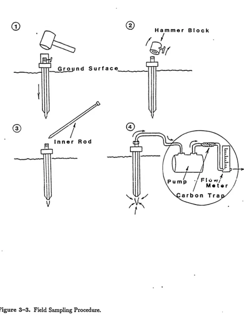
developed by WaUingford et al. (1988). The instrument is shown in Figure 3-3. To take a

vapor-phase sample, a 5-cm hole was drilled to a depth of 1.3 m, and then the probe was

inserted and poimded another 15 cm into the groamd. A diaphragm pump equipped with

a Teflon-silica diaphragm was then attached to the top of the probe and soil vapor was

pimaped at a flow rate of 50 cm^ per minute for 20 minutes. After passing through the

pump, the soil vapor was passed through an activated carbon trap to remove any organic

vapors. The carbon trap was then stored on ice vmtil it could be extracted and analyzed

back at the laboratory (see sections on extractions and analysis).

Bottle-Point Isotherm.

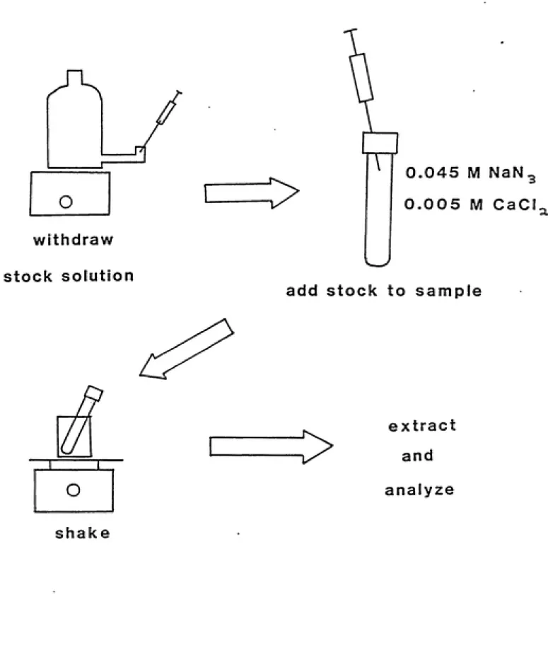
Aqueous-soUd isotherms were performed using 24-50 ml centrifuge vials. Samples were nm in pairs, and with each pair was a blank that was prepared exactly as the samples but

with no soil. Samples consisted of 20 grams of soil and 40 ml of solution. A schematic of

the bottle-point sample preparation procedure is shown in Figure 3-4.

Soil was placed in each sample vial and then a solution of calcixmi chloride and sodiimi

azide was added. This solution was 0.005 molar calcium chloride to help settle the solids

during centrifugation, and was 0.045 molar sodium aaide to suppress microbiological ac¬

tivity. This solution was added in varying amounts to each sample depending upon the

amoimt of toluene stock solution that would be added to achieve the desired final concen¬

tration of toluene.

The stock solution of toluene was prepared in a one-liter bottle. The concentration of

ͣ

Bmnci

®

0

/,

Hammer Block

/

Ground Surface

m

Inner Rod

n.

\^

I

Pump

Meter

•

into solution before use. Stock solution was withdrawn with a syringe from the septum at the bottom of the bottle and then added to the isotherm vials through the Teflon septa in the vial caps. A second syringe needle was inserted into the vial septa to allow venting of displaced air as the stock was added. This technique is believed to have reduced volatility losses because the solution was never open to the air, but was always contained within

either the solution bottle, the syringe, or a sample vial.

Diuing the sample preparation three samples were taken from the stock solution. One sample was taken at the start of the sample preparation; a second was taken after half of the vials were prepared, about 20 minutes later; and the third sample was taken after the last vial was sealed. These three samples were used to detect any change in the

concentration of the stock solution during the sample preparation procedtire.

At the end of the eqiiiUbration period, the samples were placed in a centrifuge for 30 minutes to settle the solids. Ten ml of the supematent were then removed with a syringe and then extracted with hexanes as described in the extraction section.

Bottle-Point Rate Study

The method for bottle point rate studies is very similar to that used in the isotherm experiments. The bottle point samples, however, all start with the same aqueous concen¬

tration and each is analyzed at a different time on the rate curve as the system approaches

equilibrium.

As with the isotherm experiments, 20 grams of soil sample was weighed into each of

16 50-ml centrifuge vials. Next a solution of toluene in distilled water was added to each of these samples, and also sodiimi azide to 0.25% and calcium chloride to 0.005 Molar.

The initial concentration for each sample was the same: approximately 20 mg/l. Samples

were then shaken and one was analyzed every two hours for the first 12 hotirs and then

is 515 mg/1 at 20oC. The solution was stirred for 24 hours to allow all the toluene to go

into solution before use. Stock solution was withdrawn with a syringe from the septum at

the bottom of the bottle and then added to the isotherm vials through the Teflon septa in

the vial caps. A second syringe needle was inserted into the vial septa to allow venting of

displaced air as the stock -was added. This technique is believed to have reduced volatility

losses because the solution was never open to the air, but was always contained within

either the solution bottle, the syringe, or a sample vial.

During the sample preparation three samples were taken from the stock solution.

One sample was taken at the start of the sample preparation; a second was taken after

half of the vials were prepared, about 20 minutes later; and the third sample was taken

after the last vial was sealed. These three samples were used to detect any change in the

concentration of the stock solution during the sample preparation procedure.

At the end of the equilibration period, the samples were placed in a centrifuge for 30

minutes to settle the solids. Ten ml of the supematent were then removed with a syringe

and then extracted with hexanes as described in the extraction section.

Bottle-Point Rate Study

The method for bottle point rate studies is very similar to that used in the isotherm

experiments. The bottle-point samples, however, all start with the same aqueous concen¬

tration and eaxh is analyzed at a different time on the rate curve as the system approaches

equilibrium.

As with the isotherm experiments, 20 grams of soil sample was weighed into each of

16 50-inl centrifuge vials. Next a solution of toluene in distilled water was added to each of

these saanples, and also sodium azide to 0.045 molax and calcium chloride to 0.005 molar.

ͣͣͣͣͣ

•ͣͣiiiiBRiiaip

P

withdraw

stock solution

:>

0.045 M NaN3

0.005 M CaC!

add stock to sample

>

extract and

analyze

shake

approximately 24 hours.

Samples were analyzed exactly as they were for the isotherm studies. After

centrifuga-tion, 10 ml of supematent were drawn off with a syringe and then extracted with hexanes.

Diffusion Coliman Experiments

Description of Apparatus

The diffusion experimental design is shown in Figure 3-5. The apparatus consists of

four glass coltunns exposed at one end to a chamber which is maintained at a constant

concentration of toluene in nitrogen. The other end of the soil colimans axe exposed to

a<:tivated carbon to effectively maintain the concentration of toluene at that end of the

coltmon at zero.

The chamber is a two-liter glass reaction vessel with four ground-glass ports in a

removable lid. The lid is secured to the vessel with clamps that axe easily removed, and

it is sealed with grotmd glass. One of the four ports is sealed with a Teflon plug, which

has 0.318 cm borosilicate glass tubing inserted and extending well into the chamber. This

tubing is for purging the vessel with nitrogen before beginning an experiment. The other

three ports axe fitted with groimd-glass connectors that hold the soil columns. Thus the

entire soil colmnn and connector assembly is attached by means of a groimd glass fitting.

The glass colunm is a 0.85-cm diameter glass tube 6 cm in length. The end of the tube

which is exposed to the toluene chamber is fitted with a fritted glass plug; the other end is

fitted with a ball-valve assembly that is used for inserting and removing activated carbon

samples. The carbon is placed in small glass sample vials that are covered with stainless

steel screens, which are held in place by Teflon caps. These sample vials axe placed into the

ball-valve assembly and then rotated into place. In this way the samples may be inserted

Glass Tubes

for Purging

Toluene

Stir Ring

Ball-Valve

Sampling Ports

Soil Column

Magnetic Stirrer

V ,.ͣ

mmm

Column Preparation

Both soil and glass beads to be used in the columns were first saturated with de-ionized water and then sliiixied into the glass coltimns. After weighing, the coliunns were partially dried by draining and/or blowing nitrogen through them at a very low flow rate and then they were weighed again. After the experiment was finished the columns were dried thoroughly and then weighed again. From the three weights the porosity and the

water-filled porosity could be determined.

Sampling Procedure

Samples were talcen using 0.5 grams of activated carbon in the sample vial. This vial was inserted into the ball valve assembly, rotated into place and left for one hour. At the end of the hour the ball valve was rotated back, the sample vial removed and a new vial with a fresh sample of carbon was inserted and then rotated into place. Due to the long times required for the colunms to reach equilibritmi, samples were only taken every 24-36 hovirs. Dviring the 24-36 hour period between samples 1.5-2 grams of carbon were left inserted in the ball valve to be sure to adsorb all the toluene that diffused through the end of the column dtiring that time. These larger slugs of caxbon were first saturated with water before being inserted into the apparatus. This was done to prevent a water vapor gradient occurring across the soil column between a saturated vapor chamber and a dry

slug of activated carbon.

Once an activated caxbon sample had been exposed to a colmnn for 1 hour it was extracted with carbon disulfide as described in the extraction section

Modeling Methods

A ftJly impUcit, one dimensional, finite difference model was written to simulate the

utilizes Dirichlet boundary conditions at both ends of the column. The governing equation

for the model is:

en^ = enD.^ - {Bt - eD)KH^ - P.(l - 9t)KhK,?§^ (3-1)

Combining terms gives:

1 + (1 - Ot)PsKhKp _^ jdT - dD)KH

^=De^

dt dx (3-2)

We can now define a retardation factor, Rf.

Rf = l

+---4---2---tfD "D (3-3)

and the equation becomes:

(3^)

Discretizing this equation, and dropping the vapor subscript gives:

^^ At = ^'---A^^---~~

where / represents the time step, ajid i represents the node number. Finally the equation

can be rearranged to a form which can be easily programmed in FORTRAN:

c!+i = DeAt

Ax^Rf + 2DeAi_

{cltl + cltl) +

Ax^Rf

4 EXPERIMENTAL RESULTS

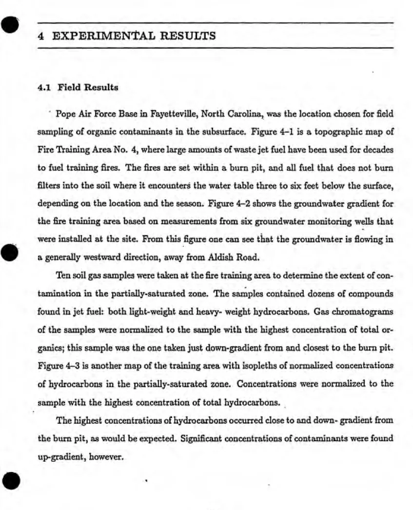
4.1 Field Results

Pope Air Force Base in FayetteviUe, North CaroHna, was the location chosen for field

sampUng of organic contaminants in the subsurface. Figure 4-1 is a topographic map of

Fire Training Area No. 4, where large amotmts of waste jet fuel have been used for decades

to fuel training fires. The fixes are set within a hum. pit, and all fuel that does not bum

filters into the soil where it encounters the water table three to six feet below the surface,

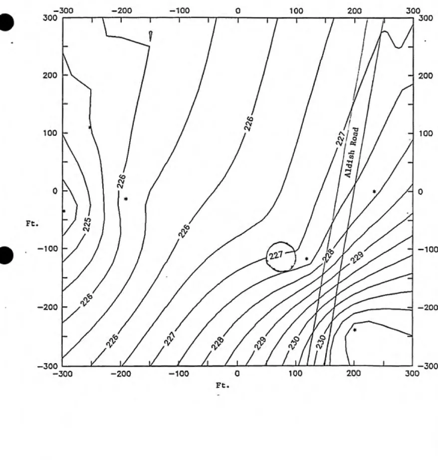
depending on the location and the season. Figure 4-2 shows the groundwater gradient for

the fire training area based on measurements from six groundwater monitoring wells that

were installed at the site. From this figure one can see that the grovmdwater is flowing in

a generally westward direction, away from Aldish Road.

Ten soil gas samples were taJsen at the fire training area to determine the extent of con¬

tamination in the partiaUy-sat\u:ated zone. The samples contained dozens of compounds

found in jet fuel: both light-weight and heavy- weight hydrocarbons. Gas chromatograms

of the samples were normalized to the sample with the highest concentration of total

or-ganics; this sample was the one talcen just down-gradient from and closest to the burn pit.

Figure 4-3 is another map of the training area with isopleths of normalized concentrations

of hydrocarbons in the partially-saturated zone. Concentrations were normalized to the

sample with the highest concentration of total hydrocarbons.

The highest concentrations of hydrocarbons occurred close to and down- gradient from

the bum pit, as would be expected. Significant concentrations of contaminants were found

Ft.

-200

-300 -100

-200 -100

300

-300

300

- 200

100

- 0

---100

---200

-300

300

Ft.

-200 -100

-300

-200

300

100

200

--300

300

- 200

- 100

^ 0

---100

- -200

-300

300

-300

300

200

-100

0

-Ft.

100

200

--300

-300

-200 -100 100 200

-200 -100 100 200

300

300

- 200

- 100

- 0

- -100

- -200

-300

300 Ft.

4.2 Sorption Study Results

Equilibrium Study

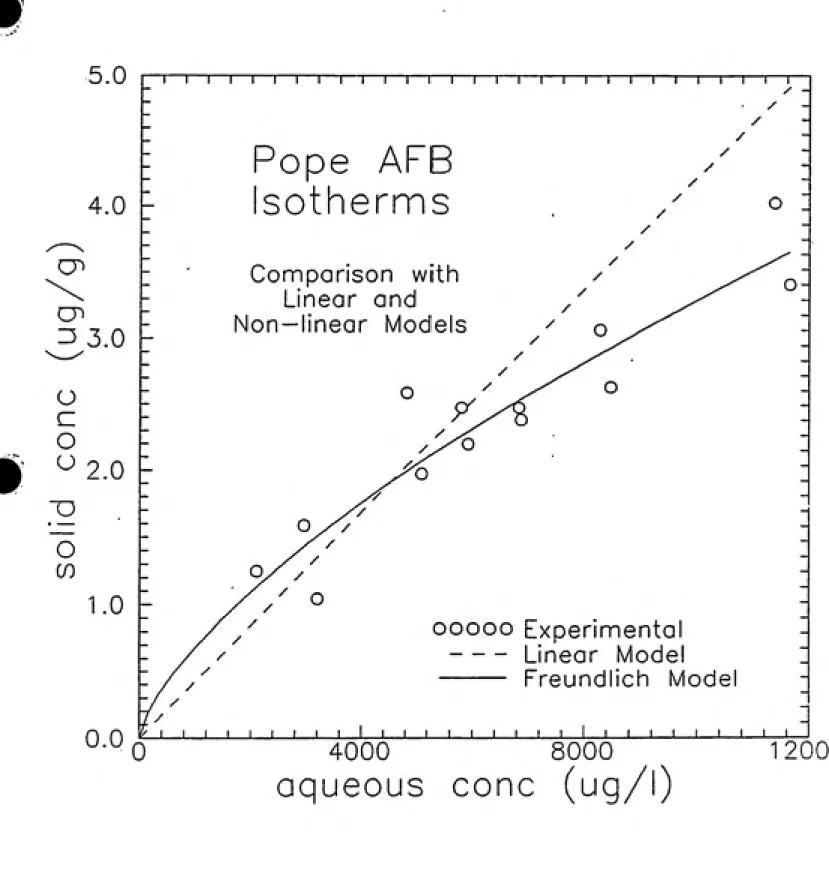
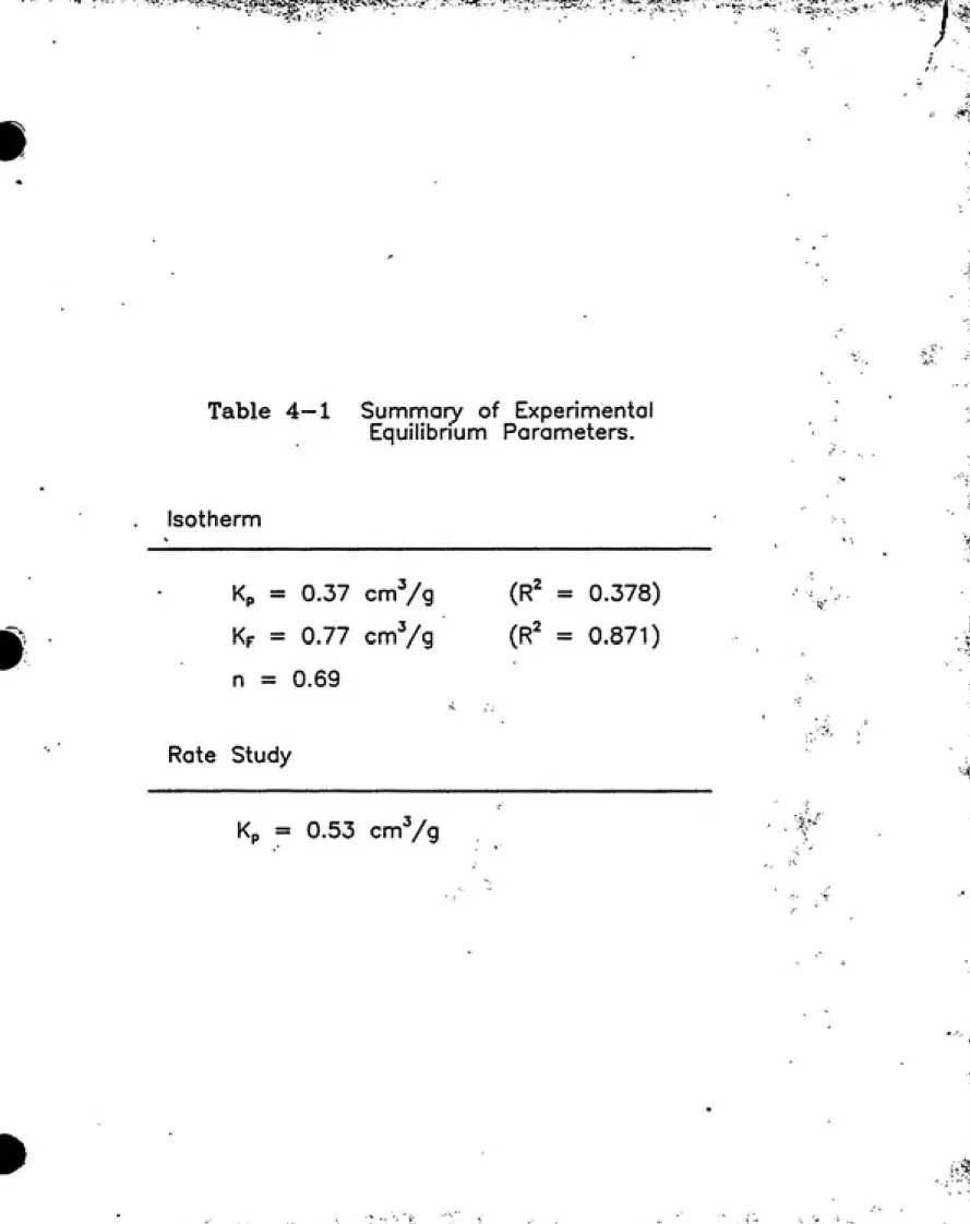
The results from the bottle-point equilibrimn study are presented in Figure 4—4. The data was fit to both linear and FVeimdlich models using a computer program written by Joseph Pedit. The linear and Fretmdlich models are graphed with the experimental data

in FigTure 4-5. The linear model gives a partition coefficient, Kp, of 0.37 cm^/g. The

correlation coefficient, i?^, for this fit is 0.378. The Freundlich model, however, produces

a much closer fit with a correlation coefficient of 0.871. The FreundHch sorption capacity

constant, Kp, is 0.0077 (cm^/g)", and the sorption intensity constant, np, is 0.685. This

data is summarized in Table 4-1.

Rate Study

The results from the bottle point rate study are presented in Figure 4-6. This graph is a plot of time versus the aqueous concentration of toluene. The samples reached an

apparent equiUbrium in approximately 24 hours, at a final aqueous concentration of 15

mg/1. The initial aqueous concentration of the samples was 19 mg/1, and Figure 4-7 is a

plot of time versus the fraction of initial toluene remaining in the aqueous phase. From this

plot one can see that at equihbrium, 20% of the toluene had sorbed onto the solid phase.

The equilibritun concentrations in the aqueous and solid phases were used to calculate a

./~*>.. 5.0 CI 4.0 O^ ^3.0 c o

/^2.0

_l 1 IT 1 1 1 1 1 1 1 r-TT

' ' ' 1 1 1 1 1 1 1 1 1 1 1 1 1 1 1 _{1 1 1 1 1 1 1 rr 1 I 1 1 i 1 1 1}

-Pope AhB

-sotherms

-Experimental

-Results -— o: -O

-o O :

-° 8

-O -o -O -O — -O

-1 -1 ._{J---L. 1 1 1 1}

J---1---L 1 1 1 I , 1 1 1 J—1 1 1 1 _{1 1 1 1 1}

-0

4000 8000

aqueous eonc (ug

1 900'^^^ v^ \_j

Figure 4-4. Results of Bottle Point Equilibriiun Study.

•

5.0 "T I 1 I I 1 I I—\—I—1—I—1—I—\—1—I—I—I—I—i—I—I—I—I—I—I—1—r

/

4.0

Cn

=3 3.0

o c

O

^2.0

O

m

1.0

Pope AFB

Isotherms

Comparison with

Linear and

Non —linear Models

0.0 J______I I I_____1_____L__J_____I_____\_____1_____I_____\_____L

ooooo Experimenta

---Linear Model

--- Freundlich Model

I I I I I I I I I I I

0 4000 8000

aqueous cone (ug

1 2000

Table 4—1 Summary of Experimental

Equilibrium Parameters.

Isotherm

Kp = 0.37 cmVg

Kf = 0.77 cmVg

n = 0.59

(R^ = 0.378)

(R^ = 0.871)

Rate Study

#

"^ 16

-]—I—I—1—I—I—I—I—I—i—I—I—I—I—I—I—I i i I—I—I—I—I—I—I—r

Bottle Point Rate Stu

-O

oo _o

Initial Conc.= 19 mg^

K. 0.53

o o

o o o

o

J____1____1____1____I____I____I I I I I I I I I I I I I I I I

0 50 100 150 200 250 300 350

Time fhr

1.00

(3 0.90

O

en

o (D

< 0.80

0.70

1—i—I—1—I—I—I—I—I—I—I—I—I—r 1—1—I—I—I—I—I—I—I—I—1—r

Bottle Point Rate Study

JD

"O

O O _O

initial Conc.= 19 nng/l

Kp = 0.53

o

o o o

o

I I I I I I i I I I I I I I I I I I I 1 I I I I I I I I I I I I I

0 50 100 150 200 250 300 350

Time (hr)

^^ex 4.3 Diffusion Column Results

Several nms were made with the diffusion column apparatus. The results of these

column experiments axe presented in Figures 4-8 through 4-13.

For each col\imn the total porosity, dx, and the gas-filled, or drained porosity, 6^, were

calculated gravimetrically. A stunmary of these properties are presented in Table 4-2. Also

in this table are the effective diffusivities calcidated for each column at steady state, and tortuosity fa<:tors. Tortuosity factors were calculated from the steady state diffusivity and

the diffusivity of toluene in pure nitrogen:

JDe = rD* (4-1)

All columns were run at constant moisture content except column 1-A. This column grad¬

ually dried out completely until 9d equaled 6t- The steady-state data is included in Table 4-2, but a graph of the transient behavior is not presented because the transient diffusion

in this column was compUcated by the drying process.

4.4 Modeling Results

The diffusion columns were modeled using the one-dimensional finite difference model described in the methods section. The porosity, drained porosity and effective diffusivity from each experimental colvuim. run were used as parameters for each successive model run. The model is capable of simulating linear partitioning of toluene between the aqueous and vapor phases, and also linear sorption from the aqueous to the solid phase. The model was

therefore run with the linear sorption constant, Kp, that was determined from the

bottle-point experiments, but could not be nm with the experimental FretmdUch parameters, Kp, and np.

160

120

O

80

CO (f)

o

40

0,

1 I I 1 I I I I I I I I I I rn I I I I I i I i I I I \ I I r

ͣ

---e---o

Column B—^

Results

soil

0T = 0.552 0D = 0.154

I I I I I I I I I I I I...___I___LJ___\___LJ___I___I___I___I___L I I I

0 100 200 300

Time (hours

/I nr\

-t-wu

200

150 sz

Z3

Li_

if) if)

O

100

50

0

"T—I—I—I—1—I—\—\—I—I—\—1—I—I—\—I—\—I—I—I—I—\—I—I—1—I—1—I—I—1—1—\—I—r

-O

Column C

Results

soil

0T = 0.572 0D = 0.249

111...I I I I 1 I I I I I I I I I I I I I I I I I I I I I

0 100 200 300 H-00

Time (hours)

1200

1000

800

O

600

% 400

D

200-T I I I 1 1 I 1 1 1 I I I I I I I i I I 1 1 I I 1 I i I I I 1 I r

-^

Column B —2

Results

glass beads 0T = 0.594 0D = 0.462

1 I I I I I I I I I I I I I I I I___l_J___I___I___I___i___I___1_1___I___I___I___I___I___I___I___L_J—I___L

20 40

Time fhours

60 80

#

90r

80

70

13 •60

_o

L^ 50

if) if)

^40

30 E

I I I I I I I I I I I I I I I I I I T~i—I—I I I I I—r

Column B —3

Results

soil

0T = 0.505

0Q = 0.265

on ri I I I I I I I I I I I I I I I I I I I I I I I I I I I I I I I I I I I I I I I I I I I I I I I I

^^0 50 100 150 200 250

Time (hours)

50

40

_c en =5 30

O

20

if)

if)

D

10

0,

1—I I I I I I I I I I I I—I—I—\—i—I—I—I I I I I—r-T—1—1—I—1—\—I—I—r

Column C —3

Results

soil

0T = 0.505 00 - 0.153

I I I I I I I I I I I I I I I I I I I I I I I I I I I I I I I I I I I I I I I I

0 50 100 150 200

Time (hours)

11111

?sn

800

700

600

ͣ

500

O

400

cn if)

^ 300

200 r

100

.1 I I I I I I I I I I I I I I I I I I I I I I I I I I I I I I I I I I I I I I I I I I I ...

-o

Column B —4

Results

glass beads 0T = 0.563 0D - 0.378

•| I I I I I I I I I I M I M I I I I I I I I I I I M I I I I I I I I I I I I I M I I I I I I I I I I I I I I I I I I I I I I I I I

0 20 40 60 80 100

Time (hours)

120 140

Table 4—2 Summary of Diffusion Column Data.

Column Steady State Dg

Column Media Length Mass Flow Qj Qq r

(cm) (^g/hr) (cm /hr)

A-1 soil 15

B-1 soil 6 C-1 soil 6

B-3 soil 6 C-3 soil 6

B-2 glass beads 6 B—4 glass beads 6

D* = 280 cm^/hr

700 233.8 0.550 0.550 0.835

155 74.0 0.552 0.154 0.264

180 53.0 0.572 0.249 0.190

84 23.4 0.505 0.265 0.083

45 21.6 0.505 0.153 0.077

1030 163.9 0.594 0.462 0.585

data. Aqueous- and solid-phase partitioning were not included in this sample run; the results from the model predict the transient diffusion through the soil column assuming that there was no loss of toluene from the vapor phase to either the aqueous or solid phases. The difference in the shape of the two curves, experimental and predicted, suggest that there is some loss of mass from the vapor phase during the transient period.

The experimentally determined linear sorption constant was included in the model and run for each column also. Figure 4-15 is a sample graph of the results of one of these runs. It was foxmd that the model utilizing the experimentally determined Hnear sorption

constant did not describe the transient colvmin behavior well for most of the column runs.

A linear sorption constant that best fit the experimental data was determined for each

column using the model, and then a simulation was nm using that constant. A sample of

%-200 150 13 _o (f) if) O 100 50 0

I I I I I I I I I I I I I I I I I I I I 1 r I I I I I I I I I I I I

-O / _ / - / / / _l 1 J ͣ i 1 I ^ r

Columnn C —

Connporison

with

Viodel

0

SOI

0T = 0.572

0D = 0.249

QOOOQ Experimental

---Model: Kp = 0

I I I I I I I I i I i I I I I I I i I I i I I...I I I I I I I I I I 100 200 300

Time (hours)

400

200

150

_o Lj_

(f)

O

100

50

0

I I I I I I I I I I I I I I I I I I I I I I I I n I I I 1 I 1 i I 1 r

- / : /

: /

:/ :i

'J

]

Columnn C —

Comparison

with

Mode

SOI

0T = 0.572

Od = 0.249

&^^^o Experimental

---Model: Kp = 0.37

I I I I I I I I I I I I I I I I I I I I I I I I I I I I I I I I I I I I I I

0 100 200 300

Time (hours)

400

200

150

sz

en

13

_o

(f) (f)

o

100

50

a

11111111111111111111111111111111111111

Columnn C —

-o

Best Fit

Linear Sorption

/

/

I r I I IZj

SOI

0T = 0.552

0D = 0.154

OOOOQ Experimental

---Model: Kp - 24.2

I I I I I I I I I I I I I I I I I I I I I I I I I I

0 100 200 500

Time (hours)

400