ACKNOWLEDGMENTS
I would like to thank my research advisor Dr. Douglas Crawford-Brown for his insight and guidance which has been invaluable to me in completing this project.
I would also like to thank Dr. Edward Chaney and Harris McMurry of the Radiation Oncology Department of North Carolina Memorial Hospital for their time and use of the resources of
the Department.
TABLE OF CONTENTS
ACKNOWLEDGEMENTS...iii
LIST OF TABLES...V LIST OF FIGURES...vi
ABSTRACT...vii
Section 1. PURPOSE...___... 1
2 . LITERATURE REVIEW...2
a. Bonner Spheres Used in Previous Studies...2
b. Neutron Production...11
3. THEORY OF NEUTRON MEASUREMENT WITH BONNER SPHERES...17
4 . MATERIALS AND METHODS...19
a. Neutron Counting Equipment...19
b. The Computer Program...24
5 . RESULTS...30
6. CONCLUSIONS...44
APPENDIX A...54
1. 52 X 5 response matrix for Bonner Spheres...26
2 . PuBe source count data...31
3. Accelerator count data...31
4. PuBe computer data, log-log smoothing...36
5. PuBe computer data, iteration...36
6. PuBe computer data, iteration-smoothing...36
7. Accelerator computer data, log-log smoothing...37
8. Accelerator computer data, iteration...37
9. Accelerator computer data, iteration-smoothing...37
10. Residuals at "best fit" steps...46
LIST OF FIGURES
Figure
1. Relative counting rate vs energy for Bonner Spheres....4
2. Cross section vs neutron energy for reactions of interest ...5
3. Various neutron integral spectra...14
4. Neutron counting system...21
5. Radiation therapy treatment room at N.C. Memorial Hospital...23
6. PuBe spectra, log-log smoothing alone...3 3 7. PuBe spectra, iteration alone...3 3 8. PuBe spectra, iteration-smoothing...34
9. Accelerator spectra, log-log smoothing alone...34
10. Accelerator spectra, iteration alone...35
11. Accelerator spectra, iteration-smoothing...35
12. PuBe "best fit" spectrum, iterative-normalized...39
13. Accelerator "best fit" spectrum, iterative-normalized...39
14. "Best fit" PuBe spectrum (histogram)...4 0 15. "Best fit" Accelerator spectrum (histogram)...41
16. Previously published neutron energy spectrum of PuBe source...42
ABSTRACT: A METHOD FOR UNFOLDING THE SPECTRUM OF NEUTRON
ENERGIES PRODUCED BY MEDICAL LINEAR ACCELERATORS by William W.
DeForest
The use of high energy linear accelerators for radiation therapy has given rise to an unexpected Health Physics
concern. These accelerators are designed to produce electrons
or photons in excess of 10 MeV. In recent years it has been noted that these accelerators are producing significant
fluences of high energy neutrons which contribute greatly to the dose equivalent received by technicians and others in
areas adjacent to treatment rooms. Proper shielding of these neutron fluences requires knowledge of the neutron spectrum at
barriers to the treatment room. The present paper presents
one method by which the neutron spectrum may be unfolded. The
method makes use of Bonner Sphere data and matrix inversion
computer codes to approximate the spectrum of neutrons
which a spectrum of neutron energies associated with neutrons produced by medical accelerators may be determined. A
technique by which to unfold neutron spectra has been of great interest to the medical physics field since the advent of high energy linear accelerators used for radiation therapy.
These high energy linear accelerators are used to provide
both electrons and, with the introduction of target materials, photons in excess of 20 MeV. Not long after these
accelerators came into use, it became evident that neutrons
were also being produced. Neutrons are produced primarily in the target and head shielding materials. These neutrons
provide no medical benefit and can be thought of as
contamination to the primary beam. A detrimental effect of the neutrons is to increase whole body dose to the patient.
Technicians, and others in adjacent areas, may also be exposed
to these neutrons due to their high penetrability and
scattering characteristics. The whole body dose equivalent
delivered to patients and others as a result of this contamination may be significant due to the high quality factors associated with neutrons.
Proper attenuation of neutron dose equivalents and
fluences is not easy to achieve, even for monoenergetic beams.
This is due to the fact that most interactions that neutrons
Because neutron reaction cross-sections change appreciably with neutron energy, the picture is still further complicated. Neutron spectra arise in accelerators due to the variety of
neutron production modes and materials in which the neutrons
are produced and interact.
Taking these points into consideration, it is evident
that proper neutron shielding is difficult to predict.
Furthermore, in order to make the attempt, knowledge of the
neutron spectrum is a necessity.
This paper will investigate one method by which an
approximation of a neutron spectrum may possibly be
determined. The method makes use of Bonner sphere data,
matrix inversion computer codes and smoothing routines to provide an estimate of the spectrum of neutron energies
produced by a source. This method then is applied to
measurements of neutron spectra produced by medical linear
accelerators.
The research involved with developing this technique was
carried out on a Siemens 20 linear accelerator located in the
radiation therapy department at N.C. Memorial Hospital.
2. LITERATURE REVIEW
2a. Bonner Spheres Used in Previous Studies
The first use of a multisphere neutron spectrometer was
•
landmark paper, five polyethelyene spheres were used with diameters of 2, 3, 5, 8 and 12 inches. After this paper, these spheres became known as Bonner spheres. Bonner et al.
used a Li(I) crystal scintillation detector located at the center of each sphere. The crystal size was kept to a minimum
(4mm in dia. and 4mm thick) to provide good gamma
discrimination. It was noted that 80% of incident thermal
neutrons are absorbed in the 1st mm of the crystal, whereas a gamma deposits only a tiny fraction of it's energy in the
entire volume of the crystal. By providing a large surface to volume ratio, the gamma discrimination effect is enhanced.
The purpose of the research by Bonner et al. was to
determine the counting efficiency of each sphere as a function
of neutron energy. In order to accomplish this, each of the spheres was exposed to a beam of monoenergetic neutrons of known fluence. Corrections were made for unequal illumination and background neutron counts. The curves that were generated were the basis for a large number of subsequent studies of
neutron spectra, and also are used in this research. These curves are reproduced here in figure 1.
Li(I) detectors will count only those neutrons that are
near thermal energies'^'^^'. This is because large
probabilities for neutron absorption in Li^, given by the
• • • fi •
absorption cross section of Li , will only occur at these
energies (see figure 2). The polyethylene spheres provide the
?2 I -~
i ""^
i
-1 o
M
2
X-u _
(B
o
X •
)K He-3 1»./,|
A Li - 6 I", alpha)
n B - 10 l», alpha)
I I 11 mil I I I iiml I I M iiitl t I I iiiiil t I I mill i i ti iiiil i i 11 mil i t 11 mil i ...
si 5 i 5 I 5 I 5 I 5 I 5 1 5 I 5
1 X 10-' 1 X 10- 1 X 10' 1 X 10' 1 X 10' 1 X 10* 1 X 10* 1 X 10* 1 X 10'
Entrgv (aV)
Cross section versus neutron energy for some reactions of interest in neutron deiection>,(2)
size, Bonner et al. found that for neutron energies above 50
keV, count rates decreased with increases in energy. Larger
spheres showed increases in count rates per unit fluence with increases in neutron energies, at least to a point. As
energies were increased further, count rates per unit fluence
dropped off quickly. In large spheres, neutrons with low energies prior to entering the sphere are captured before
reaching the Li(I) crystal. Small spheres showed decreases in
count rate per unit fluence with increases in neutron energy due to the fact that energetic neutrons were not slowed to thermal energies before reaching the Li(I) detector volume.
Bonner et al. suggested that further experiments to determine neutron energy distributions be performed with the
source to detector distance as small as possible. This
suggestion was intended to reduce the effects of background
and to increase net counting rates.
Each sphere was placed over the detector and exposed to
the neutron source. The number of interactions in the
detector then was recorded for each sphere. This number was
was equal to the sum of the number of interactions produced by neutrons in each energy interval considered by the researchers
(the total neutron spectrum having previously been divided
into discrete energy intervals).
be solved for in characterizing the neutron energy spectrum.
^ Watkins and Holeman^-^^ suggest that data from Bonner
spheres may be expressed as:
Y{i) = / A^E,i) X(E) dE(i)
^^min
Here Y(i) is the count rate (counts/s) of the detector incorporating the ith size sphere, A(E,i) represents the
response or counting efficiency (counts per N/cm') of the ith
sphere for neutrons of energy E, and X(E) represents the
actual intensity of the neutrons in the external neutron field
and m a certain energy interval E to E + dE (N/cm s). If the
neutron spectrum is divided into a discrete number of energy
intervals, the above equation also can be expressed as a
linear matrix equation of the form
y = AX (eq. 1) or equivalently
^m
^1,1' ^1,2' ^1,3' ^1,4' ••* ^1,^
^1,2' ^2,2
^3,1
Am,l' V2 ͣ^Sijn
X-X.
X-X
n (eq. 2)
In the matrix equation shown above (eq. 2) , Y-|^ through Y^^
detector/Bonner sphere coverings exposed to a neutron source.
ͣ
^11 through h^^ is the matrix of response coefficients
(counts/N/cm ) for the detector/sphere combinations, with each
row corresponding to a particular diameter of Bonner sphere
for each of n energy intervals. In other words, A^^ is the
response of the m*" detector/sphere combination to neutrons in
the n^" energy interval. X is the array of neutron energy
fluence values (N/cm^), one for each of n neutron energy
intervals. When the X values are multiplied by the
corresponding A values and the products for each row are
summed, a value of Y may be determined. This may be more
easily understood in the following form.
Yi = Ai^i(Xi) + Ai^2(^2) + Ai^3(X3) + ... A^^^, (X„)
Because the values of the A matrix are known from the
literature, and the values of Y for any detector/sphere
combination is known (determined by exposing detector/sphere
combinations to the neutron source), the object is to invert
the matrix equation and solve for the unknown elements of the
X array. Solving for the X array gives the neutron fluence in
each energy interval and hence the neutron spectrum.
Many techniques can be used to invert and solve a system
of n linear equations and n unknowns, an example being through
Gaussian elimination. Gaussian methods for solving n
equations and n unknowns are well known. Using Bonner
spheres, the maximum number of equations and unknowns would be
seven, since seven spheres are commercially available.
equation), it has drawbacks.
The first drawback is that only seven energy intervals would be generated for the spectrum. This causes many
significant and important features to be omitted from the
spectrum, such as the high energy (but low count rate) tail
and narrow width energy peaks.
A second drawback of standard Gaussian techniques is that often negative results are obtained. This occurs in matrices
of high singularity. Singularity refers to the condition
often encountered in matrix equations where there is only one
discrete solution array to the equation. This solution may
be a very sensitive function of the values of Yj^. Small
fluctuations in the values of Y (due to counting statistics),
or small uncertainties in the values of A, may greatly
influence the values of X that must be assumed in order to
reproduce the values of the Y array. The Gaussian method
obtains values of X without regard to the magnitude or sign of
values in the X array. In order to solve the matrix equation
for the unknown array, Gaussian methods may incorporate
negative values into the solution array. In this case, these
negative values would correspond to negative neutron fluence
values for some neutron energy intervals, a situation which is
physically impossible. The need therefore arose for an
alternative iterative technique to be used, one which did not
Rather than using a response matrix of 7 energy
intervals, a larger number of neutron energy intervals in the response matrix would give much better energy resolution of
the resulting neutron fluence array (X). Any number of response coefficients can be generated for detector/Bonner sphere combinations by determining the counting efficiency of
each detector/sphere combination in monoenergetic neutron
sources of known fluence. Conventional iterative techniques
(such as Gaussian elimination) cannot be used in this case, however, due to the fact that there could be more unknowns
than equations (i.e. n may exceed m). Fortunately there are other mathematical techniques, known as recursion methods, which yield an approximation of the array X when n exceeds m. These techniques start with an initial solution to X, which usually is obtained by multiplying the array Y by the inverse
of the matrix A or by the identity matrix. The technique then slowly modifies X in a systematic manner (specific to the
recursion method) until the product of A and X reproduces Y to a predetermined degree. At each point in the recursion, a check is made to ensure that all values of X cohere to certain
restrictions such as physical plausibility (no negative
values). The code then modifies the elements of X to yield a
new solution, which is compared to the previous solution (and
so on through a large number of iterations). An unfortunate problem with recursion routines is that the final solution for X often depends upon the choice of the initial solution. At
modified iterative techniques seem to be the best choice for
solving the resulting matrix of linear equations produced by Bonner sphere data in which n exceeds m. A methodology for such a technique was put forth in a paper by Watkins and
Holeman^"^^ . Many authors have used a variety of techniques to
unfold neutron spectra based on count rates obtained from
Bonner Spheres. A 52 x 7 response matrix for A(E,i) has been
computed by Hansen and Sandmier^^^ containing response
coefficients for 52 energy intervals and for 7 sizes of
spherical polyethylene coverings. Watkins and Holeman^ ' used
a modified Scofield-Gold iterative technique, which
approximates the unknown elements of a determined system of
simultaneous equations using the diagonal elements of a
diagonal matrix as the initial solution to X.
Various other iterative methods for solving equations similar to (1) and (2) have been summarized by Nachtigall and
Burger^^' and Patterson and Thomas^^^. Lowery and Johnson^^^
used a computer code based on the Scofield-Gold technique,
known as SPUNIT, which was developed at Pacific Northwest
Laboratories by Brackenbush and Scherpelz. This code gives
non-negative solutions to the spectrum and smoothing of the spectrum could be added to the results. It is a technique such as this that has been used in the present research.
2b. Neutron Production
Modes of neutron production and data on neutron yields
from electron linear accelerators have been discussed by many
Neutrons are produced in the accelerator primarily when
it is operated in the photon mode. In this mode, the photons
are produced by introducing a target metal into the electron
beam produced by the accelerator. Photons (X-rays) are
produced as bremsstrahlung radiation in the target. These
high energy photons then interact with the heavy nuclei shielding materials surrounding the accelerator head to
produce fast neutrons.
The primary mode of production of neutrons is through the (^,n) reaction with lesser contributions from the (y,2n) and (y^pn) reactions. Direct production of neutrons in either photon or electron modes is possible from the (e,n) and
(e,e'n) reactions if the energy of the electron is
sufficiently high. The production of neutrons from these
electron reactions is smaller by a factor of over two orders
of magnitude than the photoneutron reactions (due to the fine
structure constant modified by several other factors). The production of neutrons from these electron reactions for the
most part can be neglected ^^'.
For medical linear accelerators operating at less than 45 MeV, neutron production is largely due to reactions occurring
in the giant photonuclear resonance, also known as the giant
spectrum in the giant resonance has two major components. The
first and largest component is the evaporation spectrum. In
this component, neutrons are generated by compound nuclear
formation. The nucleus may be thought of as being heated or
excited by the photon, the result being that neutrons at the
highest energy levels are "boiled out" of their potential
well. The (8,2n) separation energy occurs well within the
giant resonance for most shielding materials and therefore
contributes a significant number of neutrons to the total
neutron fluence. One would think that protons, alphas, or
other charged particles would be ejected from the nucleus from
the absorption of a photon as well. This does not occur,
however, because in the giant resonance sufficient energy is
not imparted to charged particles (such as protons) to
overcome the coulomb barrier for the elements of concern. The
yield of photoneutrons may be thought of as being proportional
to the convolution of the (K^ri) cross section and the
bremsstrahlung spectrum '^.
The smaller component of the photonuclear giant resonance
arises by the direct or photoionization process. In this
process, one neutron acquires all of the photon's energy; the
kinetic energy of the neutron then becomes equal to the
photon's energy minus the binding energy of the neutron in the
nucleus. The neutrons produced in this fashion are of much
higher energy than those produced by the evaporation process.
Figure 3.
I I I I I I p
0.1
C (M^l
Various neutron integral spectra showing both accelerator primary spectrum and spectrum after passing through shielding. The Cf-252 spectrum is shown for comparison. Data are from
this direct ejection of the neutron to occur, it is thought
that the angular distribution for the emerging neutrons is
slightly peaked at 90° to the incident photon (8)(10)^
Neutrons are produced inside the head of the accelerator
and penetrate iostropically. Although the shielding
incorporated into the head attenuates photons well, it does little to attenuate the fluence of neutrons. The only
significant dose equivalent attenuation is from energy losses
by the neutrons, this being due to inelastic scattering and
(n,2n) reactions. This effectively reduces the energy and
quality factor of the neutron.
Inelastic scattering occurs only at neutron energies
above the lowest excited states of the shielding material; 0.6
- 0.8 MeV for lead, and 0.1 MeV for tungsten. Obviously
tungsten is better for reducing the energy of neutrons. This
reduction in energy provides a corresponding reduction in dose
equivalent^^^^.
The (n,2n) reaction provides a minimal energy loss equal
to the binding energy of the neutron in the nucleus.
Unfortunately, it also provides two low energy neutrons of
about equal energy that contribute greatly to the low energy
neutron fluence in the treatment room (8)(^°).
After passing through a certain distance in any shielding
material, essentially all the neutrons in the spectrum have
had their energies reduced below the lowest excited state of
the shielding materials. At these energies, inelastic
Neutrons then may penetrate great distances through shielding
materials in the head with no further energy loss or
attenuation of dose equivalent.
The preceding discussion reviewed some of the factors that provide the source of neutrons in the treatment room.
The intensity of neutrons from this source as a function of
the distance from the accelerator head can be described by the inverse square law. There is, however, a second component comprised of thermal neutrons which have scattered inelasticly
(and elasticly) off the inside walls of the treatment room.
The fluence of these low energy neutrons is essentially
constant throughout the room. This thermal neutron fluence is
related to the fast neutron fluence by
P = K(Q/S)
where: ^ is the thermal neutron fluence, Q is the fast neutron
fluence, S is the inside surface area of the treatment room
and K is a constant related to the type of shielding used in
the head of the accelerator ^ '.
It has been found that photons are always more
penetrating than neutrons for the energy ranges of interest in
a medical accelerator. While producing photons of 20 MeV, the
average energy of the neutron spectrum emerging from the
accelerator head is never much above 1 MeV. If a therapy room is constructed of enough concrete to sufficiently attenuate the photons produced, the neutrons will also be modified and
captured by the large hydrogen content of the concrete. The
doorways and any other penetrations to the room, (ducts,
conduits, etc.)- In these areas, neutrons may easily scatter
to areas unprotected by the massive concrete walls (
ͣ
'-°) .
3. THEORY OF NEUTRON MEASUREMENT WITH BONNER SPHERES
Currently, methods used to calculate neutron shielding
for therapy rooms have been rules of thumb and educated
guesses. Little is known about the spectrum of neutron energies given off by accelerators or how this spectrum changes as the neutrons pass through various shielding materials. Exact methods for deteirmining required neutron
shielding, therefore, are available but rarely used. It is
extremely important that barriers be devised to absorb
neutrons and/or reflect neutrons back to the treatment room.
It is necessary to know the spectrum of neutron energies
in order to properly determine the nature of shielding needed. It is equally important to know how the spectrum changes as
neutrons pass through shields of various constructions. In this way it will be possible to develop a series of equations
to take the guess work out of neutron shielding for medical
linear accelerator facilities.
In order to determine neutron spectra, a series of
different sized Bonner spheres are often used. Although most
researchers have used Bonner spheres to moderate the neutrons,
many types of detectors, placed at the center of the sphere to
scintillation detector, which is a thermal neutron detector,
is a good choice. Upon absorption of the neutron, the
Li (n,oc)H reaction takes place, releasing an alpha particle. The track length of the alpha is sufficiently short to deposit
all of it's energy in the crystal. The amount of energy
released in the crystal will be in the neighborhood of 4.7 MeV
and will be the same for each neutron absorbed. This release
of energy results in a pulse. The electrical pulses from the
Li(I) detector located at the center of each sphere then would
all be of the same height regardless of the energy of the
interacting neutron. The only information gained from each of
the detectors therefore is a count rate. As Li(I)
scintillation detectors will also record photons interacting in the crystal, a means of discriminating between neutrons and
photons must be addressed. This is particularly important since most neutron fields are accompanied by an appreciable field of photons. The small (4mm x 4mm) size of the Li(I)
crystal helps in this respect. Photons, with their low LETs,
will deposit only a tiny fraction of their energy in the detector. This will result in a very small pulse size
compared with the neutron pulse size. By properly setting
counting thresholds, or by using similar methods, it is
possible to successfully count only the neutron pulses and
discriminate against pulses produced by photons. Problems arise only when high photon fluences yield significant pile
Bonner spheres provide the function of thermalizing fast neutrons. Neutrons that are sufficiently thermalized by the
sphere, but not absorbed in the sphere, then will be absorbed
in the Li(I) crystal according to the intrinsic detection
efficiency of the crystal at that neutron energy.
4. MATERIALS AND METHODS
4a. Neutron Counting Equipment
A series of four Bonner spheres manufactured by Ludlum
was used in this research to establish neutron spectra. The sizes of the spheres were: 3", 5", 8", and 12" in diameter.
A bare detector was also used as one of the detector/sphere
combinations. The Li(I) crystal, light pipe, and PM assembly
were also obtained from Ludlum.
A coaxial cable, designed to carry both the signal and the high voltage for the detector, was connected to the PM tube with a type C connector. The other end of the coaxial
cable was hooked to a Ludlum signal splitter, designed to
split the high voltage and the signal. High voltage was supplied to the splitter and hence the PM tube by a separate
HV supply (manufactured by Power Designs). Leaving the
splitter, the signal travels via coaxial cable to an Ortec pre amp set on 500 pF. The pre amp was hooked via coaxial cable
to an Ortec amplifier set on a gain of 20. Output of the amp
was then hooked up to a Northern Multi Channel Analyzer (MCA).
chosen in preference to a scaler to aid in discrimination
between neutron and photon pulses. Typically, photon
discrimination is a difficult task with Li(I) crystals (used
for neutron measurements) since it involves minute adjustment and readjustment of sensitive discriminator and threshold
settings. Discrimination of photon counts from neutron counts
is easily accomplished visually with the MCA. The low photon detection efficiency of the Li(I) crystal results in a low,
prominent compton shoulder seen on the MCA. The neutron
counts, however, are at much higher channel numbers due to nearly complete energy absorption of the secondary alpha. The
neutron counts also form a prominent peak, so total neutron
counts are easily obtained by integrating under this peak by setting regions of interest on the MCA or by plotting the
peaks and integrating by hand.
It was decided that the component system and it's ability
to deliver neutron counts needed to be tested. The
detector/sphere combinations were exposed to a uniform field
of neutrons (and photons) emanating from a PuBe source located at the Physics Department at UNC. Each sphere was exposed to
the PuBe source for 10 minutes and counts were obtained. The
data obtained were interpreted by setting up a matrix similar to eq. 2 and solving using a computer program described in the
next sub-section. This test was initially intended only as a test of the neutron counting system. It was later decided to
Figure 4
Diagram of neutron counting systen
-Bonner Sphere
PH tube
high voltage
ignal splitter || f
pre-amp
signal
MCA
- NIM bin
\:::^i}
described in 4b. as a test of the code's ability to solve
matrix equations of various sizes.
The neutron counting system was taken to the Radiation
Therapy department at N.C. Memorial Hospital and set up in the
therapy room containing the Siemens 20 linear accelerator.
The configuration and position of the equipment is shown in
figure 5. The detector/sphere setup was placed approximately
1.3 meters off the floor directly between the head and the
door to the maze at approximately 2 meters from the head. The
accelerator was set to deliver 18 MeV photons. Each
detector/sphere combination was exposed to photons and
neutrons resulting from identical runs on the accelerator
delivering 400 rads to an imaginary patient. No phantom
material was added to intercept the beam as this would only
serve to increase photon scatter and potentially decrease
neutron fluences through elastic scattering and radiative
capture in hydrogen.
Pulse height spectra were obtained for each accelerator
run. Neutron counts for each detector/sphere combination were
determined through integrating the neutron pulse height
spectrum by hand. This was done because the photon continuum
was of much greater energy and height than is normally
encountered in neutron spectroscopy due to photon pile-up, and
assumptions had to be made as to the shapes of some of the
neutron peaks in order to correctly subtract off photon
counts. The neutron peak was sitting on top of the high
#
Figure 5.
Diagram of radiation therapy treatment room at N.C. Memorial Hospital
containing linear accelerator showing position of Bonner Sphere detectors.
generator
-- accelerator head
Bonner spheres- I h
photon counts, the high energy slope of the photon peak was assumed to be exponential in nature, and photon counts were
subtracted off using valley to valley averaging.
4b. The Computer Program
The data obtained from the PuBe source were at first evaluated using standard matrix inversion (Gaussian
elimination method). Using this method, negative fluences
were obtained in some of the 5 energy intervals. It was
summized that a possible reason for these results was the highly singular nature of the matrix equation. It was also
noted that the response curves for the 8" and 10" spheres were
extremely similar in nature (fig. 1). That is to say, the
curves were linearly dependent (i.e. theresponse varied with energy at approximately the same rate). When solving matrix
equations, linear dependence between two equations heightens
problems encountered with singularity and thereby increases the probability of obtaining negative results. In an attempt
to solve future problems of singularity, it was decided that
the 10" sphere would not be used and the bare detector would
be used as the fifth detector/covering combination (at this
time computer codes based on Gaussian elimination methods were
still being used in this research).
In order to resolve the problem of negative fluences, and to obtain a more detailed neutron spectrum, a recursion
approach in which n exceeded m was adopted. Available data in
the response matrix. A, included estimates of the response in
table 1).
The unknown element in the system of linear equations to solve for is the neutron fluence (X) in each of the 52 energy intervals. As mentioned before, conventional computer codes which solve for the unknown elements by inversion cannot be used in this case since the number of unknowns is larger than
the number of equations.
There was a necessity, then, for a computer code to be written based on the Scofield-Gold iterative technique.
The Scofield-Gold iterative technique basically operates like other iterative techniques in that it successively alters (in
some consistent manner) the elements of the solution array (in
this case X) until closest agreement between Y and the product
of A and X is found. The computed solution array (X) then is
at best a possible close approximation of the true solution
array, with other approximate solutions being possible. It is possible to determine in a quantitative manner how close to
the true solution array (Xrp) the computed approximation (Xq)
is by calculating the difference between Y and the product of
A and X^,. An additional computer code was written to
calculate this difference with each iteration. The computer
code written for the present research replaces the computed values of the solution array (in this case the approximated
neutron spectrum X^,) back into the matrix equation (equation
2) and computes the left hand side of the matrix equation (see equation 2). This new calculated product is labelled as the
interval N energy Bare 3« 5" 8" 12" (&V) sphere SDhere SDhere SDhere 1 l.OE-2 0.1220 0.1059 0.0540 0.0156 0.0024 2 1.6E-2 0.1220 0.1087 0.0560 0.0162 0.0025 3 2.5E-2 0.1220 0.1140 0.0588 0.0171 0.0026 4 4.OE-2 0.1180 0.1225 0.0639 0.0185 0.0029 5 6.3E-2 0.1160 0.1446 0.0712 0.0207 0.0032 6 l.OE-1 0.1140 0.1530 0.0824 0.0240 0.0037 7 1.6E-1 0.1100 0.1787 0.0975 0.0285 0.0044 8 2.5E-1 0.1020 0.2050 0.1141 0.0333 0.0051 9 4.0E-1 0.1160 0.2326 0.1327 0.0386 0.0059 10 6.3E-1 0.1100 0.2560 0.1480 0.0433 0.0065 11 1.0 0.0840 0.2701 0.1605 0.0479 0.0071 12 1.6 0.0760 0.2809 0.1710 0.0517 0.0080 13 2.5 0.0680 0.2853 0.1818 0.0541 0.0082 14 4.0 0.0600 0.2872 0.1897 0.0572 0.0088
15 6.3 0.0520 0.2880 0.1971 0.0598 0.0091 16 l.OEl 0.0420 0.2877 0.2033 0.0617 0.0096 17 1.6E1 0.0360 0.2847 0.2094 0.0647 0.0100 18 2.5E1 0.0280 0.2800 0.2150 0.0675 0.0105
predicted counts). The squared difference between the newly computed left hand side (P) of the matrix equation and the actual left hand side of the matrix equation (in this case the measurements Y) is taken as the residual. This calculation is performed for each of the 5 equations and the residuals summed after each iteration. The computed solution array with the lowest summed residual would be the best approximation of the
solution array, or the "best fit".
The iterative technique must have some initial solution array (X) from which to start. This initial array could be provided, based on educated guesses about the neutron
spectrum, as input, could be calculated by the computer
program using the product of Y and the inverse of A, or could
be obtained by multiplying Y by the identity matrix. It was
decided to take the latter course since there was no
information on which to base an initial guess about the
neutron spectrum.
In summary, then, the recursion code used in the present study begins with an initial approximation to the neutron
spectrum. This approximation is obtained by multiplying the Y array (i.e. the data array) by a diagonal matrix, D. In the initial step of the recursion, X is set equal to the product of Y and D, then is multiplied by A and the product compared to Y (i.e. the residual is computed). The elements of D then
are adjusted by the recursion routine to new values, and a new
solution to X is obtained. These adjustments occur by
element of the previous solution array (X), with the change
producing the largest decrease in residual being selected at each point of the iteration. This process continues through a large number of iterations (1500), with the elements of D
changing with each iteration. The result is a total of 1500
approximations to X, each with an associated residual.
Log-log smoothing also is added to each approximation of the X
matrix before the residual is computed. This smoothing simply causes the histogram of X (which contains 52 energy intervals)
to become less subject to large changes in the number of neutrons in adjacent energy intervals. Log-log smoothing is
included to preclude the development of a wildly fluctuating
curve. A more or less smooth neutron spectrum is expected.
Log-log smoothing is applied during each loop of the recursion routine to each element of the X array, X(n), as well as to X(n+1) and X(n-l). This serves to take erratic jumps out of the curve and give a potentially more reasonable spectrum. The program was written to continue through 1500 successive approximations of the X matrix (lines 41 through 118 of the computer program in appx. A).
Each time through this iteration the program takes the
current value of each element of the fluence array X and
multiplies it by the corresponding response coefficient (from matrix A) in a given energy interval for each detector
sphere/combination. Summing these products together for each
detector/sphere combination, an array analogous to the
The elements of this predicted count array are placed into an array named P (lines 85 - 91 of the computer program in appx.
A)
The value of the elements of the P array, when compared
to the value of the elements of the Y array, provides a test
as to how closely the solution array (X^^) is able to reproduce
the elements of the Y array. A residual array may then be computed from the squared difference between the elements of the P and Y arrays for each detector/sphere combination. This residual array is labeled array R in the program code (lines
92 and 93 of the computer program in appx. A). The total
residual for each loop of the recursion routine may then be
determined as the sum of the elements of the R array (one
value for each detector/sphere combination). These total residuals for each loop are stored as elements of array AL, a
vector array of 1500 elements (one for each loop of the
recursion routine). From the information in this array, the
step which contains the best approximation of the X matrix
could be determined by searching for the lowest residual.
There is much debate in the physics community as to which recursion routine, if any, is best for solving matrix
equations for neutron spectra. For this reason it was decided that in addition to running the iterative-smoothing routine
(which includes both recursion and smoothing), both the
iterative and smoothing routines alone would be applied
independently to the data. This led to the development of
which was applied to both sets of data (the PuBe and
accelerator data). The iterative routine alone is able to solve the matrix equation (2) for the values of X although
discontinuities in the spectrum might result. It was felt
that the log-log smoothing routine alone might also
approximate the solution to the matrix equation. The
smoothing routine could accomplish this by successively
smoothing the initial spectrum as produced in lines 19 through
40 of the computer program (appx. A), although the final shape
of the spectrum would be heavily influenced by the kind of
smoothing employed. It was also not clear whether the use of
smoothing alone would allow convergence onto a solution in an
efficient manner or would lead to a physically realistic solution spectrum (i.e. the elements of the X array).
5. RESULTS
Total counts within the neutron peak for each of the five
detector/sphere combinations exposed to the PuBe source are
outlined in table 2 (integration by the MCA). The reader
should note that the data from the 10" sphere as well as the bare detector are omitted. This is because no data were
gathered for the bare detector, since problems with the linear
dependence of the 8" and 10" spheres data had not yet been
noted during the course of the research.
The total neutron counts under the peak for each of the
detector/sphere combinations exposed to the accelerator follow
valley-to-TABLE 2
PuBe source data, 10 min. counting time for each
detector/sphere combination.
Poly sphere coverina Counts
3" 642
5" 1088
8" 1497
12" 1214
TABLE 3
Accelerator data, 400 rads delivered to each detector/sphere,
counting times equal.
Poly sphere coverina Bare
B" 5" 8" 12"
Counts
5,875
63,000 42,725 7,900
valley averaging).
Both sets of data then were input into each of the three
forms of the program {smoothing alone, iteration alone,
iteration plus smoothing) as elements of the Y matrix. Through analysis of the residual array output data for
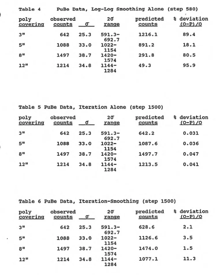
computer runs made on the PuBe source data it was determined that the best approximation of the X (neutron fluence) matrix
was to be found at step 580 of the recursion loop for the log-log smoothing only routine, and at step 1500 for the iteration
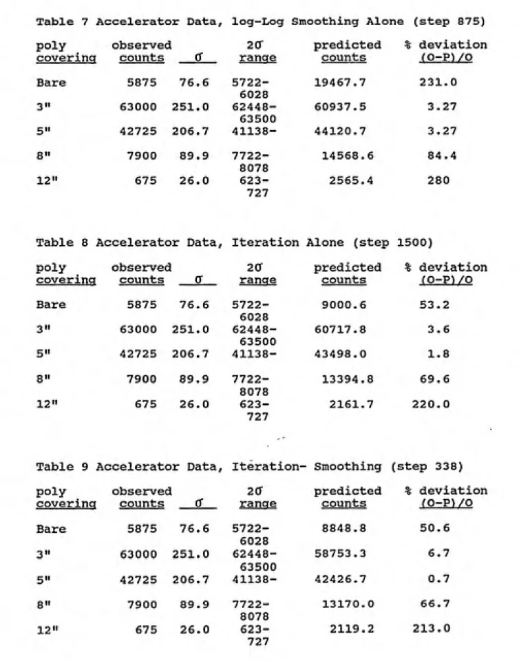
only and iteration-smoothing routines. For runs of the
computer programs utilizing the accelerator data it was found
that the best approximation of the fluence matrix was to be
found at step 875 of the recursion loop for the smoothing only routine, step 1500 for the iteration only trial, and step 338
for the iteration-smoothing trial. The X matrix was plotted
at each of these steps. Spectra were printed at additional steps to gain an understanding as to how the recursion
routines successively approximated the X matrix. The reader should see figures 6 thru 11 for plots of these X matrices
(neutron spectra). The program also output the value for the
P (predicted Bonner sphere counts) array at all "Best Fit" steps (tables 4,5, 6, 7, 8, 9) to determine how well the X array is able to reproduce the Y array by visually comparing
the P array to the Y array.
The reader may refer to tables 4 through 9 for data on
observed counts, predicted counts, standard deviation of
V o c « 3 « C
spectra ot Sb^B 1, 580, 1500
/^
1DD
-ͣ ͣ I ͣ I ' I ͣ I ' I ͣ I ͣ 1 ͣ I ͣ I ' T 'T-TTTT I I ) ) M *T' ! M
1 3 5 7 9 11 13 15 17 19 21 23 :S 27 29 31 33 35 37 ;» 41 43 45 47 49 51
st-p 1
neutron energy Interval
Bt<9p 580-"&Mt Fit" Btep 1500
Figure 7. u Z. 91 V < c D o SI 1.5 1.4 -\ 1.3 1.2 1.1 1 0.9 0.8 0.7 0.6 0.5 0.4 0.3 -0.2
0.1 -I
0
PuBe DATA - Iteration Only
Spectro at Steps 1, 580. 1000, 1500
eeSSgeaBBD
^ M I I t I I I I
M-*-1 ' M-*-1 ' I ' I ͣ I ' 1 ͣ M ' 1 I I' I ' I ' I ' I ͣ I ͣ I I I ' I ' I •' I ' 1 ' I ' I ' 1 ' 1 3 5 7 9 11 13 15 17 19 21 23 25 27 29 31 33 35 37 39 41 43 45 47
neutron energy interval
Step 1 + step 5S0 --- step 1500-Best Rt
1 ' I
t> c o o c a 2 0 C»^ 1.3 i.a 1.1 1 0.9 0,.3 0.7 0.6 0.5 0.4 d.3 0.2 0.1 0
Spectra <3t steps 1. 530, 1SOO
roDnDnoDanDDDDnaa
' I
ͣ
I
ͣ
r ' I
ͣ
1
ͣ
I
T! M M M i ' I U M ' M rM
ͣ
ͣ
1 ' I
ͣ
I
ͣ
I
ͣ
;
ͣ
1 3 5 7 9 11 13 15 17 19 21 23 ^ 27 29 31 33 35 37 39 41 43 45
I
47 49 51
.step 1
neutron ervergy intefvai
ͣ
»- Btep 580 Bt«p 1S00
Figure 9.
4^ £ «? 2 o 3 O Z
ACCELERATOR DATA - Smoothing Alone
Spectra » Steps 1, 875, ItJOO. 2600
1 3
-+- Step 1
5 7 9 11 13 15 17 19 21 23 25 27 29 31 33 35 37 39 41 43 45 47 49 51
— Step 1000 —V— ^t^P 2500
Neutron Energy Intefvo!
ͣ
a e c
g o
if
2 0
I
steps 333 & 1S00
Btisp 1 SOO-Swt Ftt
neutron energy Intetvat
fsifsp 3o&
Figure 11.
E
o
z-5
«)
3
O
ACCELERATOR DATA- Iteration 8c Smoothing
steps 1. 338. 1000
»9 9(^-»^»y<^»i^»y<<j'»^<y»^»<}»'^
tep 1000 step 1
Table 4 PuBe Data, Log-Log Smocsthing Alone step 580)
poly observed 2(y predicted % deviation
coverina counts 642 or ranqe 591.3-counts 1216.1 fO-P)/0
3" 25.3 89.4
692.7 5" 1088 33.0
1022-1154
891.2 18.1
8" 1497 38.7
1420-1574
291.8 80.5
12" 1214 34.8 1144-1284
49.3 95.9
Table 5 PuBe Data, Iteration Alone (step 1500)
poly observed 20- predicted % deviation
coverina counts 642 (J ranae 591.3-counts 642.2 fO-P)/0
3" 25.3 0.031
692.7 5" 1088 33.0
1022-1154
1087.6 0.036
8" 1497 38.7 1420-1574
1497.7 0.047
12" 1214 34.8 1144-1284
1213.5 0.041
Table 6 PuBe Data, Iteration-Smoothing (step 1500)
poly observed 20r predicted % deviation
coverina counts 642 0" ranae 591.3-counts 628.6 (0-P)/0
3" 25.3 2.1
692.7 5" 1088 33.0
1022-1154
1126.6 3.5
8" 1497 38.7 1420-1574
1474.0 1.5
12" 1214 34.8 1144-1284
Table 7 Accelerator Data, log-Log Smoothing Alone (step 875)
poly observed
coverincT counts 0" Bare 5875 76.6
3" 63000 251.0
5" 42725 206.7 8" 7900 89.9
12" 675 26.0
Table 8 Accelerator Data, Iteration Alone (step 1500)
20^ predicted % deviation
rancre counts (0-P)/0
5722- 19467.7 231.0
6028
62448- 60937.5 3.27
63500
41138- 44120.7 3.27
7722- 14568.6 84.4
8078
623- 2565.4 280
727
poly observed 2(y predicted % deviation
coverina counts 5875 0 rancre 5722-counts 9000.6 (0-P)/0
Bare 76.6 53.2
6028 3" 63000 251.0
62448-63500
60717.8 3.6
5" 42725 206.7 41138- 43498.0 1.8 8" 7900 89.9
7722-8078
13394.8 69.6
12" 675 26.0 623-727
2161.7 220.0
Table 9 Accelerator Data, Iteration- Smoothing (step 338)
poly observed 2G predicted % deviation
coverina counts 5875 (S ranae 5722-counts 8848.8 (0-P)/0
Bare 76.6 50.6
6028 3" 63000 251.0
62448-63500
58753.3 6.7
5" 42725 206.7 41138- 42426.7 0.7 8" 7900 89.9
7722-8078
13170.0 66.7
12" 675 26.0 623-727
of predicted counts (P array) for the PuBe source data and the
accelerator data.
Referring to table 1, it is quickly noted that the width
of the energy intervals, ie, 0-1, 1-2, etc., is not consistent
throughout the range of neutron energies presented. The
energy intervals continually widen going from interval number
1 to 52. For this reason, the graphical shapes of the "best fit" neutron spectra as presented in figures 5 and 8 are
misleading. The visual features on these graphs are more a
function of neutron energy interval width than actual neutron
fluence at any given energy. The reader may refer to figures
12 and 13 (probability density distributions) of the
respective "best fit" spectra normalized to energy interval
width. Here the fluence obtained for any interval was divided
by the width of that interval in eV. To give the plots still
more meaning, the respective spectra were plotted against a
consistent energy scale (figures 14 and 15).
These plots were developed by normalizing fluences obtained in
figures 12 and 13 respectively in particular energy intervals
of interest and plotting them against a common normalized
scale. Figure 16 shows the PuBe neutron spectrum determined
by Anderson and Neff using a fast neutron spectrometer,
employing pulse shape discrimination, and utilizing a single
stillbene crystal ^-^^ ^ . Figure 17 shows figure 14 superimposed
with the Anderson and Neff spectrum. The Anderson and Neff
igure . pyBe DATA — Iterative, Normalized
?
11
o 3
2
Step 1600-~e«s»t nr
3 5 7 9 11 13 15 17 19 21 23 25 27 29 31 33 35 37 39 41 43 45 47 49 51
neutron energy intervcl
Figure 13.
%
'—'ͣ^ *»» =
« o c
t-*"—'
a c
2
C
ACC, DATA — Iterative, Normalized
step 1S00-"Best Fit"
I ͣ I ͣ I ' I ' I ' 1"! 1 ' I I I ' I ͣ I ' I ' I ' I ' I ' I ͣ I ' I ͣ I ' I ' I
Figure 14 n
BEST FIT" PuBe SPECTRUM
1"^
o» o
2.8
2.6
2.4
2.2
2
1.8
1.6
-1.4
1.2
1
0.8
0.6
0.4
0.2
-0
^+
0
Q2.5
94
a 6.3
flrrrr
T"
8
Q16
-T-12
-0 25
16 20
1^
24 28
neutron energy In MeV
> -^
D
m
II
h-fflS.
[]
"T
20 40 60
-•
Figure 16.
t
6-flU
X
o
Ui
z
Ui
>
4-S
2-0-J
j'^-.^T.
n EMUUIONS
\ STILBENE
W
\\
1 I 1 { *
K^'^
K
1 i I I
4-6 8 10
NEUTRON ENERGY (M*V)
Neutron energy spectrum of Pu-Be source M-59I
containing 30 g of Pu. ^^^^
I'm
2.8 2.6 2.4 2.2 2 1.8 1.6 1.4 -1.2
1 0.8 -0.6 0.4 0.2
0
0
e-4-& NEFF
12.5 [14
---tiJ 6.."i
^PTTT
8
n 16
m25
24
----1---1---n---\---r 12 16 20
Neutron Energy Ln eV
The Anderson and Neff spectrum is broken into energy intervals to
correspond to this study. The relative intensities in these energy intervals
were calculated from Anderson and Neff data and the absolute intensity in each
interval calculated by setting the absolute intensity in the 1.0 - 2.5 MeV interval equal to that obtained in the present study.
Present study Anderson & Neff
total number of neutrons as computed by the computer codes used in this research as a means of comparison. The
significance of these plots will be discussed in later sections of this paper. j
6. CONCLUSIONS
Through a review of the data presented, it is evident
that the log-log smoothing routine operating in the computer
program alone provides the worst solution to the matrix
equation of the three program trials. This conclusion can be
arrived at by looking at the % deviation columns in tables 4
and 7. In other words, the smoothing routine yields a
solution spectrum with large residual errors compared to other
routines.
There is a difference in the spectral shapes produced by the smoothing alone and iterative alone routines when
comparing spectra at their respective "best fit" steps (i.e.
the iteration that produces the lowest residual error). This
can be explained by the fact that each time through the
recursion loop, the log-log smoothing routine shapes the curve
in a logarithmic fashion (see figures 6 and 9). The smoothing
routine then, is merely logarithymicaly altering the previous
X array during each iteration. The "best fit" spectrum from
the smoothing routine alone has no obvious physical meaning
but it is interesting to note how close this simple method
In computer program trials with both sets of data, the neutron spectra produced with the iterative alone and
iterative-smoothing techniques are very similar. The
iterative-smoothing trial "best fit" spectrum appears as a smoothed version of the iterative "best fit" spectrum.
It is interesting to note that for both PuBe and
accelerator data the iterative alone routine solution was better than the iterative-smoothing solution, this conclusion being arrived at by looking at residuals for the "best fit"
steps (table 10). The log-log smoothing routine was added to
give more realistic results, as a smooth (continuous) shape was expected, and to help in the approximation of the solution array. It would seem, however, that the smoothing routine may prove more a liability than an asset in solving the matrix
equations, at least as far as residual errors are concerned.
The smoothed spectrum is, however, more physically realistic. The iterative routine, operating in the computer program
with the smoothing routine disabled, leads to somewhat
conflicting observations. Looking at the PuBe data at step 1500 ("best fit") in table 5 and figure 7 it is noted that the routine is solving the matrix equation excellently (with very small % deviation). Whether or not it is solving for the
actual neutron spectrum is another matter, since many
solutions may be available. As a test of the ability of the
code to reproduce data obtained by more precise measurement
methods, the calculated PuBe spectrum in it's normalized form,
Table 10 Residuals (array AL) Incurred at "Best Fit" Steps
Program Trial Residuals
PuBe-Smoothing Alone 3177352.0.
PuBe-Iteration Alone 0.0996
PuBe-Iteration-Smoothing 20935.6
Accelerator-Iteration Alone 47978479.2
PuBe spectrum as reported by Anderson and Neff^ ^ in the
energy regions of dosimetric significance (figure 16).
The computed spectrum, however, extends to energy levels far
in excess of the spectrum reported by Anderson and Neff and
appears to be quite unreasonable with respect to those higher energies. In this regard it may be concluded that the current versions of the computer routines tend to "flatten" the
spectrum, pushing the spectrum to higher than reasonable
energies.
The iterative routine operating alone solves the matrix equation for both the PuBe data and the accelerator data
better than the other methods, considering the amount of residual (table 10) and the % deviation (tables 3 and 6).
Also, it solves the PuBe matrix equation nearly exactly while
leaving much to be desired with the accelerator matrix
equation. This can be seen by comparing the % deviation in tables 5 and 8. Still, the accelerator spectrum (figure 15) would appear to be qualitatively reasonable given what is
known about the moderation of neutrons in the head and walls
before reaching the detector/Bonner sphere combination have undergone many interactions in the concrete walls of the
therapy room and have lost energy through elastic collisions
with hydrogen in the concrete. Still, some higher energy
neutrons would have been expected, and their absence indicates
a potential problem with the method.
A possible problem associated with the accelerator "best
fit" spectra as presented in figures 10 and 11 is that there
is no low energy tail. This tail would be expected to be present and quite prominent due to the low energy neutron
fluence which is thought to be quite uniform in the treatment
room. As noted for the PuBe source, the computer routines
tend to flatten the spectrum, also pushing the spectrum to
higher energies. This would not, however, account for the complete removal of the low energy tail. Keeping this in
mind, it is easy to understand why the spectra as presented in
figures 13 and 15 are preferred. These figures, particularly
figure 15, give a more understandable representation of the
spectrum including the low energy tail.
Note the extended high energy tail seen in figures 14 and 15 for the PuBe source and accelerator and the over estimation
(by the computer program) of the 12" detector/sphere
combination seen in tables 8 and 9. A possible reason for the
over estimation of counts in the largest sphere size (for the
accelerator data) is that reported response coefficients in
the A matrix are included for neutron energy intervals in
These energy intervals are found in steps 48 through 52 (table 1). The iterative routine may try to fit neutron fluences into these energy inteirvals, thereby overestimating the count of the 12" poly sphere detector (which is the most responsive detector to neutrons of these energies) thereby extending the
computed spectrum to energy levels higher than are actually
occurring. The iteration routine then may effectively take some low energy fluences and push them into higher energy
levels. This effect of spectrum extension caused by the presence of response coefficients in excess of peak neutron energies in the matrix equation may also be occurring in the computer runs made on PuBe data, although no over estimation
of the 12" detector/sphere size is seen.
In order to test the possibility that inclusion of high
energy response coefficients might be moving neutrons from low to high energies, the codes were run with and without response
coefficients at high energies. The effect of spectrum
extension or shifting mentioned above would probably be more
pronounced for the PuBe data than the accelerator data if this
is in fact occurring. This is because the PuBe spectrum
naturally extends to a much higher energy range than the
scattered fluence from the accelerator. A test run was
made on both sets of data with all response coefficients for
neutron energy intervals higher than the realm of possibility omitted (higher than the upper energies of the particular
neutron source). A test run of the computer program on the
intervals 48-52 omitted produced exactly the same spectrum with the same residual at the "best fit" step as computer runs
made with those intervals included. Trial runs made on the
PuBe data with the response coefficients for neutron energies
in excess of 16 MeV deleted failed to converge onto a
solution. Clearly, response coefficients cannot simply be
omitted as tried here. Future studies might focus on a method
for dealing with the problem of unreasonably high energies in
the response matrix.
It is clear that the neutron counting system presented in this paper gives reasonably good data and performs reliably,
in the sense that residual errors between Y and AX can be made
quite small. What is not so clear is whether the computer program gives reasonable shapes to the neutron spectra. The relatively good qualitative fit of figure 14 (the normalized
"best fit" PuBe spectrum) to the PuBe spectrum reported by Anderson and Neff (figure 16) in the region of dosimetric interest shows that the unfolding method presented at least has some merit and bears further investigation. Looking at
the computed accelerator spectrum again (from the last
section) we may note that the counts for some detector/sphere
combinations predicted using the iterative only routine fell
far from the actual counts in those detectors. This, in
combination with the high residuals, would lead us to believe
that this best fit spectrum, in fact, fits rather poorly. One
must bear in mind, however, two important points. The first
observed and predicted counts, and the second is that the
accelerator "best fit" spectrum predicts counts in four
detector/sphere combinations quite well. If the spectrum
reproduces the measurement data for four out of five
independent linear equations, the spectrum cannot be too far
from being a reasonable approximation.
Assumed losses of fluences in the low energy range and
over-estimations in the high energy range remain significant
features. Table 11 displays neutron quality factors relative
to fluence and energy ^-'
ͣ
•^' . Loss of neutron fluences in the
near-thermal energy range is not that critical, as this is
where quality factors are lowest. Over estimations of the
high energy range would only lead to more conservative
calculations, as this is where quality factors are highest.
For the most part, however, neutron fluences per unit energy
above 100 eV in the calculated accelerator spectrum are
extremely small, and are nearly non-existent above 250 eV.
This could have important implications in shielding
calculations, which require information on the higher energy
neutrons.
In order to obtain better estimates of neutron spectra in
the future using techniques similar to the one presented in
this paper, several points may be raised. First, the presence
of response coefficients above the range of expected neutron
energies warrants further investigation. Another is that
other smoothing routines may be tried, log-log smoothing
(linear-Table 11
Neutron quality factors at various energies
Neutron Energy Quality
fMeV) Factor
thermal 3
0.0001 2
0.005 2.5
0.02 5
0.1 8
0.5 10
1.0 10.5
2.5 8
5.0 7
7.5 7
10 6.5
10-30
Relative
N/cmVs
linear) approach is one possibility. Lastly it may be possible to give the computer program a better initial
starting spectrum. This a priori spectrum would have to be
one of a shape which is highly expected from past measurements or theoretical considerations. Other authors have suggested
this approach and have used it^^'^ '. The value of this
approach is questionable, however, since it is not clear what spectrum should be assumed at the start and how that choice
affects the results. A possible advantage to such an
approach, however, is that it might be more efficient in terms
of computer time, as fewer recursion loops would be necessary
(assuming you chose the right initial spectrum).
The unfolding process as presented in this paper seems to give qualitatively reasonable results for both PuBe and
accelerator data. With further work aimed at resolving the problems associated with spectrum shifting and choice of
initial spectrum, this process may be used in conjunction with
existing and future shielding calculations to provide adequate
barriers to neutron contamination in linear accelerator
APPENDIX A
The Computer Program
(as modified to handle the accelerator data) C data input section and echo out
1 IMPLICIT REAL*8 (A-H), INTEGER (I-N) 2 REAL*8
3 A(5,52),X(52),Y(5),B(52,52),AT(52,5),W(52),Z(52),R(5),
4 P(52),D(52,52),AL(1000)
5 DO 20, 1=1,5
6 READ(5,FMT=10)(A(I,J),J=1,52) 7 READ(5,FMT=30) Y(I)
8 30 FORMAT(F7.1)
9 WRITE(6,FMT=15)(A(I,J),J=1,52)
10 15 FORMAT(IX, 9F7.4)
11 10 FORMAT(9F7.4) 12 20 CONTINUE
13 WRITE(6, FMT=40)(Y(I),1=1,5)
14 40 FORMAT(5F10.4)
C transpose of A matrix 15 DO 50, 1=1,52
16 DO 50, J=l,5 17 AT(I,J)=A(J,I)
18 50 CONTINUE
C building of initial spectrum 19 DO 60, 1=1,52
20 WBT=0
21 DO 70, J=l,5
22 WBS=AT(I,J)*Y(J) 23 WBT=WBT+WBS
24 70 CONTINUE 25 WB(I)=WBT 26 60 CONTINUE
27 DO 80, K=l,52 28 DO 90 1=1,52
29 BT=0
30 DO 100, J=l,5
31 BS=AT(I,J)*A(J,K) 32 BT=BT+BS
33 100 CONTINUE 34 B(I,K)=BT 3 5 90 CONTINUE 36 80 CONTINUE 37 N=0
38 DO 110, 1=1,52
39 X(I)=WB(I) 4 0 110 CONTINUE
C beginning of recursion loop 41 DO 500, N=l,2500
C smoothing of each spectrum in loop 42 DO 120, J=2,52
45 END IF
46 IF (X(J+1) .LE. 1.0) THEN 47 X(J+1)=1.1
48 END IF
49 IF(X(J) .LE. 1.0) THEN 50 X(J) =1.1
51 END IF
52 X(J)=DEXP(DEXP((DL0G(DL0G(X(J-1)))+4*DLOG(DLOG(X(J)))+
53 DL0G(DL0G(X(J+1))))/6))
54 120 CONTINUE
C printing of various spectra 55 IF (N .EQ. 1.0) THEN
56 PRINT*, 'N =•,N 57 DO 121, 1=1,52
58 PRINT*, •X',I,'=',X(I)
59 121 CONTINUE
60 END IF
61 IF (N .EQ. 500) THEN 62 PRINT*, "N =',N
63 DO 122, 1=1,52
64 PRINT*, •X',I,'=',X(I)
65 122 CONTINUE
66 END IF
67 IF (N .EQ. 875) THEN 68 PRINT*, 'N =•,N
69 DO 123, 1=1,52
70 PRINT*, 'X',1,'=',X(I)
71 123 CONTINUE
72 END IF
73 IF (N -EQ. 1000) THEN
74 PRINT*, 'N =•,N 75 DO 124, 1=1,52
76 PRINT*, 'X',I,'=',X(I) 77 124 CONTINUE
78 END IF
79 IF (N .EQ. 1500) THEN 80 PRINT*, 'N =',N
81 DO 125, 1=1,52
82 PRINT*, 'XSI, • = ',X(I)
83 125 CONTINUE
84 END IF
C calculation of predicted counts in bonner spheres
85 DO 130, K=l,5 86 P(K)=0
87 DO 140, M=l,52 88 Z(M)=0
89 Z(M)=A(K,M)*X(M)
90 P(K)=Z{M)+P(K)
91 140 CONTINUE
C calculation of residuals each bonner sphere 92 R(K) = (Y(K)-P(K) )**2
93 130 CONTINUE
C printing of predicted counts
95 PRINT*, 'N =',N 96 DO 145, K=l,5
97 PRINT*, 'P(K)',K,'=•,P(K)
98 145 CONTINUE
99 END IF
C calculation of total residual for loop
100 AL(N)=0
101 DO 150, K=l,5 102 AL(N)=AL(N)+R(K) 103 150 CONTINUE
C calculation of new spectrum (X array)
104 DO 160, 1=1,52
105 WVT=0
106 DO 170, J=l,52 107 WVS=B(I,J)*X(J) 108 WVT=WVT+WVS 109 170 CONTINUE 110 WV(I)=WVT
111 160 CONTINUE
112 DO 180, 1=1,52 113 D(I,I)=X(I)/WV(I)
114 180 CONTINUE
115 DO 190, 1=1,52 116 X(I)=D(I,I)*WB(I) 117 190 CONTINUE
118 500 CONTINUE
C printing of final X array
119 PRINT*,'X' 120 DO 200, 1=1,52
121 PRINT*,'X',I,~=^,X(I)
122 200 CONTINUE
C printing of residuals
123 PRINT*, ' ' 124 PRINT*, 'AL', 125 DO 550, N=l,2500
126 PRINT*, "AL" ,N,'=\AL(N)
127 550 CONTINUE