M E T H O D O L O G Y A R T I C L E
Open Access
Mixture SNPs effect on phenotype in
genome-wide association studies
Ling Wang
1*, Haipeng Shen
1,3, Hexuan Liu
2and Guang Guo
2,4,5Abstract
Background: Recently mixed linear models are used to address the issue of “missing" heritability in traditional Genome-wide association studies (GWAS). The models assume that all single-nucleotide polymorphisms (SNPs) are associated with the phenotypes of interest. However, it is more common that only a small proportion of SNPs have significant effects on the phenotypes, while most SNPs have no or very small effects. To incorporate this feature, we propose an efficient Hierarchical Bayesian Model (HBM) that extends the existing mixed models to enforce automatic selection of significant SNPs. The HBM models the SNP effects using a mixture distribution of a point mass at zero and a normal distribution, where the point mass corresponds to those non-associative SNPs.
Results: We estimate the HBM using Gibbs sampling. The estimation performance of our method is first
demonstrated through two simulation studies. We make the simulation setups realistic by using parameters fitted on the Framingham Heart Study (FHS) data. The simulation studies show that our method can accurately estimate the proportion of SNPs associated with the simulated phenotype and identify these SNPs, as well as adapt to certain model mis-specification than the standard mixed models. In addition, we analyze data from the FHS and the Health and Retirement Study (HRS) to study the association between Body Mass Index (BMI) and SNPs on Chromosome 16, and replicate the identified genetic associations. The analysis of the FHS data identifies 0.3% SNPs on Chromosome 16 that affect BMI, including rs9939609 and rs9939973 on theFTOgene. These two SNPs are in strong linkage
disequilibrium with rs1558902 (Rsq=0.901 for rs9939609 and Rsq=0.905 for rs9939973), which has been reported to be linked with obesity in previous GWAS. We then replicate the findings using the HRS data: the analysis finds 0.4% of SNPs associated with BMI on Chromosome 16. Furthermore, around 25% of the genes that are identified to be associated with BMI are common between the two studies.
Conclusions: The results demonstrate that the HBM and the associated estimation algorithm offer a powerful tool for identifying significant genetic associations with phenotypes of interest, among a large number of SNPs that are common in modern genetics studies.
Keywords: Bayesian variable selection, Genome-wide association studies, Gibbs sampling
Background
Genome-wide association studies (GWAS) have success-fully identified genetic loci association with complex diseases and other traits. SNPs identified by traditional GWAS can only explain a small fraction of the heri-tability, due to the strict multiple-comparison significance requirement when testing each SNP individually. For
*Correspondence: lingw@email.unc.edu
1Department of Statistics and Operation Research, University of North Carolina-Chapel Hill, 27514 Chapel Hill, USA
Full list of author information is available at the end of the article
example, Vissher [1] discussed 54 loci associated with height which only explained 5% heritability; [2] described 32 loci associated with Body Mass Index (BMI) which explained 1.45% of the variance in BMI. More recently, [3] used mixed linear models (MLM) to simultaneously take into account all the SNPs, which is shown to alleviate the missing-heritability issue.
In this study, we extend the work of [3] to identify the subset of SNPs that are significantly associated with the phenotype of interest, instead of assuming all the SNPs are associative, through a Hierarchical Bayesian model
(HBM). Similar to [3], all SNPs are considered simulta-neously to estimate the heritability, instead of one by one as in the traditional GWAS, hence our HBM also helps to capture missing heritability. Different from the authors in [3], we assume that the SNP effects are distributed as the mixture of a point mass at zero, for those non-effective SNPs, 6 and a normal distribution for those associative SNPs.
Our proposed Hierarchical Bayesian model (HBM) can be represented using the following set of Eqs. 1 and (2). Eq. 1 follows the same set-up as [3]: Y is the n × 1 response vector which corresponds to the individuals’ phenotype in our study, Xis the design matrix for the fixed effects, W is the standardized genotype matrix, and the vector b contains the N SNP random effects, where thejth element is the random effect corresponding to thejth SNP and is assumed to follow the mixture dis-tribution as in (2), depending on the latent indicatorIj, j=1,. . .,N:
Y=Xβ+Wb+, (1)
where
bj
=0, if Ij=0,
∼N0,σb2, if Ij=1, and Pr(Ij=1)=p, j=1,. . .,N. (2)
One key contribution of our HBM is its capability of automatically selecting significant SNPs while simultane-ously incorporating all the SNPs. Eq. 2 is the technical rea-son behind the selection feature, which can be intuitively understood as follows. Imagine that each SNP is coupled with one Bernoulli indicatorIjwith success probabilityp, and all theN Bernoulli indicators are independent. The SNPs then fall into two categories, where the first category contains those withIj = 1, which are the 100×p% asso-ciative SNPs with effects following a normal distribution, while the second group includes the remaining SNPs with Ij=0, who have zero effects. The selection of the associa-tive SNPs is achieved through identifying the SNPs with Ij= 1, which are chosen to be those with the largest pos-terior probability of being 1, through the HBM algorithm as described below:
The HBM Algorithm
InitializeChoose starting values of
β(0),b(0),I(0),p(0),σ2
e(0),σb2(0)
. Iterate
1. Drawβ(t)fromP
β(t)|Y,b(t−1),σ2
b( t−1)
,σe2(t−1)
.
Pβ|Y,b,σb2,σe2∝exp −2σ12
e(y−Xβ−Wb)
t
(y−Xβ−Wb)exp −1 2βtk−1β
, wherekis a
k×kmatrix withσa2on the main diagonal and 0
everywhere else, withkbeing the dimension ofβ.
2. Drawb(t)from
Pb(t)|Y,β(t−1),I(t−1)
j =1,σb2( t−1)
,σe2(t−1)
andbjis
set to zero ifIj(t−1)=0.
Pb|Y,β,Ij=1,σb2,σe2∝ exp − 1
2σ2
e(y−Xβ−WIb)
t(y−Xβ−W Ib)
×
exp −1 2bt
D−2
q
b, whereWIare the columns ofW
corresponding toIj(t−1)=1, andDis the diagonal
matrix with the main diagonal asσb2and the dimension
asq=j
Ij(t−1)=1
3. DrawIj(t)fromP
Ij(t)|Y,β(t),bj(t),σb2(t−1),σe2(t−1)
.
PIj|Y,β,bj,σb2,σe2= p×φ(bj,σp×φ(bj,σb)
b)+(1−p)×φ(bj,σ), where
φstands for the standard normal density.
4. Drawp(t)from
Pp(t)|Y,β(t),I(t),b(t),σ2
b( t−1)
,σ2
e(t−1)
. Pp|Y,β,I,b,σb2,σe2∝
pqj=1Ij(1−p)q− q
I=1Ijpα0−1(1−p)β0−1
5. Drawσe2(t)fromP
σ2
e(t)|Y,β(t),I(t),b(t),σb2( t−1)
. Pσ2
e|Y,β,I,b,σb2
∝(σ2
e)−n/2exp
−(y−Xβ−Wb2)σt(2y−Xβ−Wb)
e σ
2
e−a1−1exp
−b2 1
σ2 e
.
6. Drawσb2(t)fromP
σ2
b( t)|Y
,β(t),I(t),b(t),σe2(t)
.
Pσ2
b|Y,β,I,b,σe2∝σb2
−1Ij=1/2exp
−
1Ij=1(bj)2
2σb2 σ 2
b
−a2−1exp
−b2 2
σ2 b
.
7. Repeat from Step 1 to Step 6 until convergence.
the joint posterior density of the hierarchical regres-sion model with a factorized form and minimizes the Kullback-Liebler distance between the factorized form and the full posterior distribution. Although this method is fast to compute, the accuracy of prediction depends on how well the factorized form approximates the poste-rior distribution of the hierarchical model [5]. Developed a Bayesian variable selection regression algorithm to solve the hierarchical model. They adopted several strategies to improve computational performance, for example, they used marginal associations of the SNPs on the traits as the initial screen step for the latent indicatorIjin (2) [6]. This indicates that the distribution of the random effectbj is similar to the marginal estimates of the SNP effects on the traits.
In this study, we modify the standard MCMC algo-rithm based on the stochastic search algoalgo-rithm proposed by [7]. The algorithm directly samples the parameters from their posterior distributions and obtain the infer-ences for the parameters. Because the number of SNPs is large, each iteration of the algorithm involves matrix inversion with the dimension being the number of SNPs. To reduce computation time, we modify the algorithm by sampling the random effects bj conditional on the indicatorIj. The modified algorithm significantly reduces computation time, especially when the number of SNPs is large and the mixture probability pis small, while is still able to identify the significant predictors accurately. Detailed description of the algorithm will be stated in Section “Methods”: Method. We also implement several computing tricks so that the algorithm can be used to esti-mate models with the number of SNPs in the order of 100,000 (Section “Example 2”).
Our HBM is first applied to analyze simulated data sets in Section “Simulation studies” to show that the proposed algorithm is able to identify the SNPs that are significantly associated with the phenotype and correctly estimate the model parameters as well as PVE, which is defined as the proportion of total genetic variance over total phenotypic variance:
PVE= σ
2
g
σg2+σ2
(3)
whereσg2is the total genetic variance which equalsσb2in (2) times the number of SNPs. The total phenotypic vari-ance is the sum of the genetic varivari-anceσg2and the variance of the error terms ofin (2), denoted asσ2.
We also compare HBM with the Genome-wide Com-plex Trait Analysis (GCTA) proposed by [3]. The basic concept of GCTA is to fit the effects of all the SNPs as random effects using a mixed linear model (MLM). Note that the MLM is a special case of our HBM when p = 1. It is shown in our studies that if a large number of SNPs have small/noisy effects on the phenotype, the MLM tends to over-estimate the PVE while the HBM is still able to correctly estimate it. We present in Section “Real data set results” two real data applications through the Framingham Heart Study [8] and the Health and Retire-ment Study [9], where we study the association between the SNPs on Chromosome 16 and the phenotype body mass index (BMI). We are able to identify associative SNPs on theFTO gene which are consistent with earlier find-ings in the literature and replicate the results in the two studies.
Results and discussion
Simulation studies
The performance of the HBM and MLM is illustrated using two simulated examples with the identical simu-lation settings but different number of random effects. Example 1 (Section “Example 1”) considers 10,000 ran-dom effects, while Example 2 (Section “Example 2”) has 100,000 random effects and is closer to the scale of real GWAS. Each example also consists of two simulation cases: in Case 1 the random effects follow a mixture distri-bution of a point mass at zero and a normal distridistri-bution, while in Case 2, the random effects follow a mixture of two normal distribution with one of the two has a very small variance, trying to mimic scenarios with a large number of small/noisy effects on the phenotype.
For both simulated examples, genotype information of the individuals from the Framingham Heart Study (FHS) is used as input matrix. Detailed description of the FHS data is provided in Section “The Framingham heart study”.
Example 1
In this example, we randomly select 10,000 SNPs on Chro-mosome 16 of the FHS data and use them as the input genotype matrix,W. The traitYis then simulated accord-ing to the followaccord-ing model:
Y=β0+Wb+, (4)
a mean of zero and variance ofσ2. As discussed above, two simulation cases are generated as follows.
• Simulation Case 1:The random effectbfollows a mixture distribution of a point mass at zero plus a normal distribution. In this situation, the SNPs are either associated with the phenotype (whose random effects are distributed as a normal distribution) or not associated with the phenotype (whose random effects will be zero);
• Simulation Case 2:The random effectbfollows a mixture of two normal distributions with one of the two distributions has a very small variance. In practice, many SNPs might have very small/noisy effects on the complex traits [10]; hence, we are simulating those scenarios with letting some of the SNPs have noisy effects on the phenotype that are normally distributed with a very small variance.
For Simulation Case 1, we randomly select 100× p% of the SNPs as the ones associated with the pheno-type (namely, the association SNPs), and draw their ran-dom effectsb from the distributionN0,σb2, and treat the remaining SNPs as non-association SNPs with zero effects. We then fix the PVE at the predetermined value, and simulate the residualfrom the distributionN0,σ2
whereσ2
= jVar(bj)(1/PVE−1). Phenotypeyis gen-erated usingW,bandaccording to Eq. 4. For Simulation Case 2, the data set is generated in a similar way as in Case 1, with the only difference being that the random effects for the non-association SNPs are simulated from N0,σ2whereσ is a very small number (e.g.σ =0.01) instead of zero.
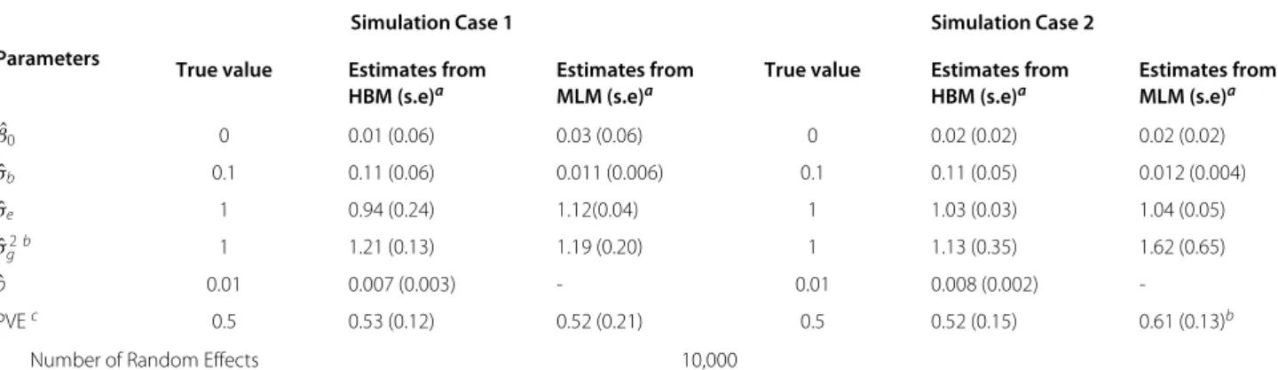
Table 1 shows the estimation results from the simulated data sets using the HBM and MLM along with the true model parameters. The estimated mixture probabilitypˆ
and the random effect varianceσˆbby the HBM are close to their corresponding true values, 0.01 and 0.1, respec-tively. This demonstrates the good performance of our estimation method. In both simulation cases, the MLM severely underestimatesσb2, as it divides the total genetic variance onto all the SNPs, instead of just the 1% associ-ation SNPs (p = 0.01), which results in underestimation of the genetic effects. In addition, in Simulation Case 2, the estimated PVE from the MLM is much larger than the true value while the HBM gives a closer PVE esti-mate. The reason is that the MLM can not distinguish the “significant” SNP effects versus those “noisy” effects due to its assumption that all random effects follow the same distribution. Therefore,σˆg2obtained by MLM would include both “significant” and “noisy” effects and thus lead to overestimation of PVE according to (3). We comment that the simulation model in this case is different from the underlying models assumed by our HBM and the MLM of GCTA. As the results indicate, the HBM is rather robust against such model misspecification.
Example 2
This simulation example is used to demonstrate the per-formance of the HBM algorithm when the number of SNPs is large (i.e. 100,000), in the order of real GWAS. We have to implement several computational optimizing strategies in order to speed up the computation on such a large number of SNPs as well as to efficiently use the computer memory.
First, in each iteration of the HBM algorithm, we need to invert a square matrix with the rank the same as the num-ber of SNPs. Instead of inverting this matrix directly, we employ the Sherman-Morrison-Woodbury formula [12], to change the matrix inversion to one that only has the same rank as the number of observations, which usu-ally is much smaller than the number of SNPs in genetic
Table 1 Example 1 - estimation results
Simulation Case 1 Simulation Case 2
Parameters
True value Estimates from Estimates from True value Estimates from Estimates from
HBM (s.e)a MLM (s.e)a HBM (s.e)a MLM (s.e)a
ˆ
β0 0 0.01 (0.06) 0.03 (0.06) 0 0.02 (0.02) 0.02 (0.02)
ˆ
σb 0.1 0.11 (0.06) 0.011 (0.006) 0.1 0.11 (0.05) 0.012 (0.004)
ˆ
σe 1 0.94 (0.24) 1.12(0.04) 1 1.03 (0.03) 1.04 (0.05)
ˆ σ2
gb 1 1.21 (0.13) 1.19 (0.20) 1 1.13 (0.35) 1.62 (0.65)
ˆ
p 0.01 0.007 (0.003) - 0.01 0.008 (0.002)
-PVEc 0.5 0.53 (0.12) 0.52 (0.21) 0.5 0.52 (0.15) 0.61 (0.13)b
Number of Random Effects 10,000
aValues in parenthesis are standard errors.bGenetic Varianceσˆ
g2is defined in the same way in [11] which equals toσˆb2×N. N is the number of SNPs whose effectbj follows theN(0,σb2) distribution.cPVE is calculated as σˆ
2
g
ˆ σg2+ ˆσ2
studies. Secondly, computation using a large number of SNPs is intensive. Analyzing large datasets of SNPs seems to be impractical on uniprocessor machines. Thus, we carry out the analysis in parallel on UNC-CH’s multi-core Linux-based cluster computing server. We write scripts to distribute the computation among multiple cores/CPUs and run multiple computing analyses simultaneously. Our study shows that parallel computing can speed up the computation by a factor of 20 on a 10-core computing node on the cluster. It takes 668.5 minutes and 158GB memory to finish the calculation for the simulated data set with 100,000 SNPs. To consider whole genome data with even more SNPs, the amount of memory and computation power of the server will be the main bottleneck.
Similar to Example 1 in Section “Example 1”, we consider the same two simulation cases. The estimation results are summarized in Table 2. Even for the larger number of SNPs, our HBM still performs well in both cases, while the same drawbacks exist for the MLM.
For Example 2 (with 100,000 SNPs), Table 3 reports the cross table results of the association SNPs identified by HBM against the truth. As one can see, the HBM can cor-rectly detect 76% and 82% of the true association SNPs for the two simulation cases respectively, and more than 99.9% of the true non-association SNPs. This suggests that the HBM works very well at detecting association SNPs with the false positive rate as low as 0.062% and 0.041%, respectively.
Real data set results The Framingham heart study
We further apply HBM and MLM to data from the Fram-ingham Heart Study [8] to study genetic associations with the body mass index (BMI). The FHS is a community-based, prospective, longitudinal study following three generations of participants.
Genotyping for FHS participants was performed using the Affymetrix 500K GeneChip array. Genotypes on the Y chromosome are not included in our analysis. A stan-dard quality control filter is applied to the genotype data. Individuals with 5% or more missing genotype data were excluded from analysis. SNPs that are on the X chro-mosomes and have a call rate≤ 99% or a minor allele frequency≤ 0.01 were also eliminated from the analysis. The application of the quality control procedures resulted in 8,738 individuals with 287,525 SNPs from the 500,000 genotype data. Genotype data were converted to minor allele frequencies for the analysis. One individual of a pair is deleted if the genetic relationship is greater than 0.025. Note that the genetic relationship between individual j and individualkis defined as in [3]:
Ajk = N1 N
i=1
(xij−2pi)(xik−2pi)
2pi(1−pi) , (5)
where xij/xik is the number of copies of the reference allele for the ith SNP of the jth/kth individual andpi is the frequency of the reference allele. After the above pre-processing, there are 1,915 unrelated individuals in the analysis.
Because the total number of SNPs in the FHS data is close to 300,000, computation is limited by the memory of the UNC server if we include all SNPs in the anal-ysis. Therefore, as a proof of concept, the 13,764 SNPs on Chromosome 16 are used in the analysis. Another reason for considering this chromosome is that it con-tains an enzyme fat mass and obesity associated protein also known as FTO. We would like to see whether the HBM can identify the SNPs that are significantly corre-lated with BMI on Chromosome 16, especially those SNPs on the FTO gene. We include the first seven Principle
Table 2 Example 2 - estimation results
Simulation Case 1 Simulation Case 2
Parameters
True value Estimates from Estimates from True value Estimates from Estimates from
HBM (s.e)a MLM (s.e)a HBM (s.e)a MLM (s.e)a
ˆ
β0 0 0.12 (0.08) 0.12 (0.13) 0 0.09 (0.09) 0.12 (0.07)
ˆ
σb 0.1 0.13 (0.01) 0.005 (0.002) 0.1 0.13 (0.05) 0.009 (0.002)
ˆ
σe 3 2.86 (1.05) 3.15 (1.45) 3 3.67 (1.13) 3.18 (1.05)
ˆ σ2
g 3 2.37 (1.34) 2.53 (2.01) 3 3.17 (2.13) 8.1 (3.25)
ˆ
p 0.003 0.0024 (0.001) - 0.003 0.0025 (0.001)
-PVE 0.5 0.45 (0.24) 0.44 (0.23) 0.5 0.46 (0.25) 0.72 (0.33)b
Number of Random Effects 100,000
Table 3 Example 2 - detection results from HBM
Simulation Case 1 Simulation Case 2
Association SNPs Non-association SNPs Association SNPs Non-association SNPs identified by HBM identified by HBM identified by HBM identified by HBM
Association SNPs 76% 24% 82% 18%
Non-Association SNPs 0.062% 99.938% 0.041% 99.959%
Components (PCs) for BMI as fixed effects in the model to eliminate genotype correlation induced by biological ancestry.
The estimation results are shown in the left panel of Table 4. We see that the estimated mixture probabilitypˆ from HBM is around 0.3%, which indicates only 0.3 per-cent of the SNPs on Chromosome 16 are associated with BMI.
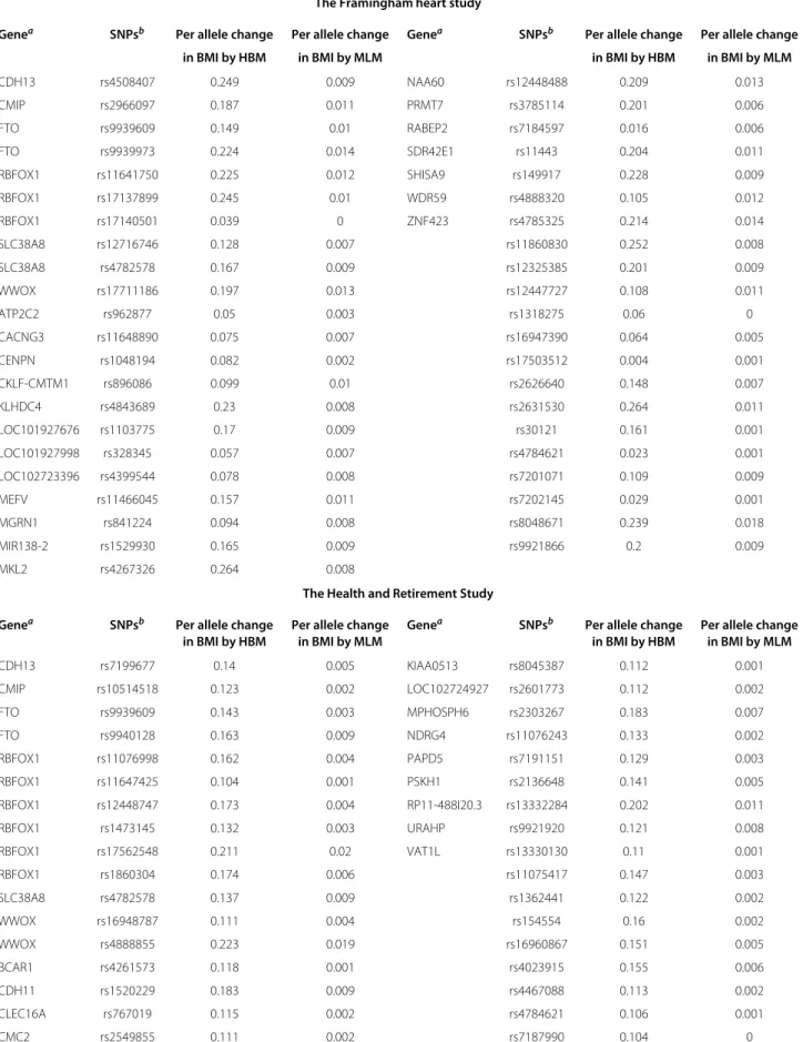
The top panel of Table 5 lists the 43 SNPs that are iden-tified by HBM as associated with BMI, which are ordered according to their names, along with the corresponding genes if available. Among these identified SNPs, the SNP rs9939609 variant has been found to be associated with obesity risk among children and adolescents of Beijing, China by [13], and with BMI and waist circumference among European- and African-American youth by [14]. The SNP rs9939973 on theFTOgene has also been found
to be related with overweight of children in Korean by [15]. These two SNPs are in strong linkage disequilib-rium (LD) with SNP rs1558902 (Rsq=0.901 for rs9939609 and Rsq=0.905 for rs9939973), which had been previously reported in a well-known GWAS [2]. The detection results can also be replicated to some extent: the three SNPs highlighted in red and the genes indicated in blue are also detected in the HRS analysis to be reported below in Section “The health and retirement study”.
The predicted allele effects on BMI (kg/m2per allele) by HBM and MLM are compared in Table 5, which are calculated as the posterior mean of the random effects under each model. The allele effect predicted by HBM is closer to the findings in the previous GWAS. As an example, we compare SNP rs9939973’s effect on BMI with rs1558902’s, both of which are on theFTOgene and are highly correlated [2], found that the per allele change in
Table 4 Real data estimation results using HBM and MLM
The Framingham heart studya The health and retirement studyb
Estimates from Estimates from Estimates from Estimates from
Parameter HBM (s.e)b MLM (s.e)b HBM (s.e)b MLM (s.e)b
ˆ
β(Intercept) 26.42 (0.29) 26.46 (0.28) 27.47 (0.07) 27.47 (0.05)
ˆ
σb 0.20 (0.09) 0.014 (0.005) 0.014 (0.009) 0.0001 (0.00002)
ˆ
σe 24.68 (0.38) 22.64 (0.41) 22.32 (0.23) 27.29 (0.41)
ˆ σ2
g 1.49 (0.40) 3.49 (0.35) 0.6678 (0.4) 0.95 (0.38)
ˆ
p 0.0034 (0.0005)c - 0.0042 (0.0004 )c
-PVE 0.06 ( 0.01)d 0.13 (0.01)d 0.026 (0.01) 0.04 (0.01)
PC1 -19.01 (44.72) -10.90 (44.15) 82.75 (33.56) 91.66 (20.10)
PC2 -18.00 (24.41) -18.27 (24.90) -15.54 (8.52) -18.41 (10.49)
PC3 2.63 (8.91) 5.65 (10.25) 26.01 (9.32) 23.01 (6.91)
PC4 -10.13 (9.11) -10.05 (9.45) 3.52 (3.24) 2.24 (6.83)
PC5 18.55 (9.44) 19.80 (9.89) 14.43 (11.14) 8.49 (6.79)
PC6 -4.75 (12.17) -4.49 (12.02) -9.77 (14.34) -19.81 (6.77)
PC7 16.06 (12.46) 13.09 (12.48) -1.21 (11.95) -2.39 (6.74)
aThe analysis is based on 1,915 unrelated persons in the Framingham Heart data set using 13,764 SNPs on Chromosome 16 to predict BMI.bThe analysis is based on
Table 5 Per allele change in BMI for association SNPs identified by HBM
The Framingham heart study
Genea SNPsb Per allele change Per allele change Genea SNPsb Per allele change Per allele change
in BMI by HBM in BMI by MLM in BMI by HBM in BMI by MLM
CDH13 rs4508407 0.249 0.009 NAA60 rs12448488 0.209 0.013
CMIP rs2966097 0.187 0.011 PRMT7 rs3785114 0.201 0.006
FTO rs9939609 0.149 0.01 RABEP2 rs7184597 0.016 0.006
FTO rs9939973 0.224 0.014 SDR42E1 rs11443 0.204 0.011
RBFOX1 rs11641750 0.225 0.012 SHISA9 rs149917 0.228 0.009
RBFOX1 rs17137899 0.245 0.01 WDR59 rs4888320 0.105 0.012
RBFOX1 rs17140501 0.039 0 ZNF423 rs4785325 0.214 0.014
SLC38A8 rs12716746 0.128 0.007 rs11860830 0.252 0.008
SLC38A8 rs4782578 0.167 0.009 rs12325385 0.201 0.009
WWOX rs17711186 0.197 0.013 rs12447727 0.108 0.011
ATP2C2 rs962877 0.05 0.003 rs1318275 0.06 0
CACNG3 rs11648890 0.075 0.007 rs16947390 0.064 0.005
CENPN rs1048194 0.082 0.002 rs17503512 0.004 0.001
CKLF-CMTM1 rs896086 0.099 0.01 rs2626640 0.148 0.007
KLHDC4 rs4843689 0.23 0.008 rs2631530 0.264 0.011
LOC101927676 rs1103775 0.17 0.009 rs30121 0.161 0.001
LOC101927998 rs328345 0.057 0.007 rs4784621 0.023 0.001
LOC102723396 rs4399544 0.078 0.008 rs7201071 0.109 0.009
MEFV rs11466045 0.157 0.011 rs7202145 0.029 0.001
MGRN1 rs841224 0.094 0.008 rs8048671 0.239 0.018
MIR138-2 rs1529930 0.165 0.009 rs9921866 0.2 0.009
MKL2 rs4267326 0.264 0.008
The Health and Retirement Study
Genea SNPsb Per allele change Per allele change Genea SNPsb Per allele change Per allele change
in BMI by HBM in BMI by MLM in BMI by HBM in BMI by MLM
CDH13 rs7199677 0.14 0.005 KIAA0513 rs8045387 0.112 0.001
CMIP rs10514518 0.123 0.002 LOC102724927 rs2601773 0.112 0.002
FTO rs9939609 0.143 0.003 MPHOSPH6 rs2303267 0.183 0.007
FTO rs9940128 0.163 0.009 NDRG4 rs11076243 0.133 0.002
RBFOX1 rs11076998 0.162 0.004 PAPD5 rs7191151 0.129 0.003
RBFOX1 rs11647425 0.104 0.001 PSKH1 rs2136648 0.141 0.005
RBFOX1 rs12448747 0.173 0.004 RP11-488I20.3 rs13332284 0.202 0.011
RBFOX1 rs1473145 0.132 0.003 URAHP rs9921920 0.121 0.008
RBFOX1 rs17562548 0.211 0.02 VAT1L rs13330130 0.11 0.001
RBFOX1 rs1860304 0.174 0.006 rs11075417 0.147 0.003
SLC38A8 rs4782578 0.137 0.009 rs1362441 0.122 0.002
WWOX rs16948787 0.111 0.004 rs154554 0.16 0.002
WWOX rs4888855 0.223 0.019 rs16960867 0.151 0.005
BCAR1 rs4261573 0.118 0.001 rs4023915 0.155 0.006
CDH11 rs1520229 0.183 0.009 rs4467088 0.113 0.002
CLEC16A rs767019 0.115 0.002 rs4784621 0.106 0.001
Table 5 Per allele change in BMI for association SNPs identified by HBMContinued
CNGB1 rs7184838 0.172 0.012 rs8045580 0.126 0.005
CNTNAP4 rs4888514 0.178 0.008 rs964933 0.114 0.001
GPR139 rs868554 0.14 0.002 rs9925215 0.119 0.005
aThe same genes are identified associated with BMI using both FHS and HRS data are shown in blue.bSNPs identified to be associated with BMI in both FHS and HRS
data are shown in red.
BMI for SNP rs1558902 is 0.39 (kg/m2) based on a total of 249,796 individuals of European ancestry using a GWAS method. It is much closer to the estimate obtained by HBM (0.224kg/m2), rather than the much-lower estimate given by MLM (0.014kg/m2). This comparison indicates that the MLM, assuming that every SNP has an effect on the phenotype, underestimates the SNP effects.
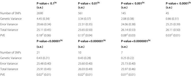
One can also see from Table 5 that the estimated PVEs are different (5.6% vs. 13.3%). In Section “Simulation studies”, we have shown that the MLM tends to over-estimate PVE if there exist many SNPs with small/noisy effects on the phenotype, which we think is also the case for the FHS data here. To demonstrate that there exist SNPs with small effects on BMI, we perform the follow-ing multi-scale analysis by varyfollow-ing the amount of SNPs on Chromosome 16 to be included in MLM and show-ing how the correspondshow-ing estimated PVE changes. We first regress BMI on every single SNP and obtain the cor-respondingp-value. Then we consider a range of varying thresholds on thep-values, and only include those SNPs with ap-value below the threshold in the MLM when esti-mating the PVE. We systematically increase the p-value threshold so that more and more SNPs that are “less” sig-nificant will be included. The idea is that as the p-value threshold increases, more SNPs with small effects on BMI will be included when estimating PVE, which will result in higher PVEs. The estimation results are presented in Table 6. The estimated PVE decreases from 18% to 1% as a decreasing number of SNPs with smallerp-values (below the thresholds from 10−1 to 10−7) are included in the analysis. The results indicate that when estimating PVE using MLM, the more SNPs with small effects on BMI are included, the higher the estimated PVE is.
In summary, the analysis of the Framingham data reveals several important empirical findings: (1) Among all the SNPs on Chromosome 16, only 0.3% of them are significantly associated with BMI according to HBM; (2) Several association SNPs identified by HBM have also been reported to be significantly related with BMI in pre-vious studies; (3) The MLM tends to underestimate the allele effect on the phenotype while the HBM estimates much closer to previous GWA study results; (4) Because the MLM includes SNPs with small effects on BMI, the estimated PVE by MLM is much higher than the estimate from HBM.
The health and retirement study
In this section, we try to replicate the results in Section “The Framingham heart study” using data from the Health and Retirement Study [9]. The HRS is a longitudinal study of Americans over age 50, conducted every two years from 1992 to 2012; it collects information on economic, health, social, and other factors relevant to aging and retirement. DNA samples were collected in 2006 and 2008. Out of the collected samples, 13,129 individuals were put into geno-typing production and 12,507 passed the University of Washington Genetics Coordinating Center’s standardized quality control process.
The HRS analysis was performed on 12,237 unrelated individuals and the 11,925 SNPs on Chromosome 16 that are common to those SNPs used in the FHS analysis of Section “The Framingham heart study”.
The estimation results are shown in the right panel of Table 3 and Table 4. We first note that the HBM esti-mates of the proportion of association SNPs are very close in the two studies: 0.34% and 0.42% for FHS and HRS respectively. Both data sets identified the same set of six genes for BMI including the well-knownFTOgene. These genes account for about 25% of the genes identified in our analysis.
Forty SNPs are identified to be associated with BMI by the HBM using HRS data set, which are listed in the bot-tom panel of Table 6. Between the two studies, the HBM identifies three common SNPs to be associated with BMI: rs4782578, rs4784621 and rs9939606 (shown in red), as well as a few common genes (shown in blue). Furthermore, SNP rs9940128 identified using the HRS data is also on theFTOgene, and has been found before to be correlated with BMI by [16,17] and [18].
Conclusion
Table 6 The Framingham Heart Study: PVE Estimation Using Proportion of SNPs Based on P-value Thresholda
P-value<0.1bc P-value<0.01bc P-value<0.001bc P-value<0.0001bc
(s.e.) (s.e.) (s.e.) (s.e.)
Number of SNPs 2690 561 145 45
Genetic Variance 4.45 (0.34) 3.34 (0.37) 2.08 (0.38) 0.86 (0.31)
Error Variance 20.66 (0.34) 22.31 (0.35) 24.06 (0.38) 25.25 (0.39)
Total Variance 25.11 (0.45) 25.65 (0.50) 26.14 (0.53) 26.11 (0.50)
PVE 0.18d(0.06) 0.13d(0.04) 0.08d(0.03) 0.03d(0.01)
P-value<0.00001bc P-value<0.000001bc P-value<0.0000001bc
(s.e.) (s.e.) (s.e.)
Number of SNPs 21 10 7
Genetic Variance 0.43 (0.21) 0.43 (0.28) 0.25 (0.22)
Error Variance 25.48 (0.40) 25.60 (0.40) 25.73 (0.40)
Total Variance 25.91 (0.45) 26.03 (0.49) 25.97 (0.46)
PVE 0.02d(0.01) 0.02d(0.01) 0.01d(0.01)
aThe analysis in the table is carried out using the GCTA software developed by [3].bP-value is obtained by regressing BMI on each single SNP.cValues in the
parenthesis are standard errors.dPVE decreases from 18%to 1%as a smaller group of SNPs are included in the analysis.
We demonstrate the applicability of our approach using both simulated and real data. The simulations are first used to show the accuracy and robustness of the estima-tion algorithm. We then analyze real data from the FHS and the HRS to identify SNPs on Chromosome 16 that are associated with the body mass index (BMI). The identified SNPs are consistent with earlier findings in the literature, and the results can be replicated across the two studies. The results from both the simulations and the real appli-cations suggest that the MLM tends to over-estimate the proportion of total genetic variance over total phenotypic variance, i.e. PVE. The reason is that the MLM assumes that all the SNPs have effect on the phenotype, including those SNPs with small or noisy effects.
Our work offers a flexible framework that can be extended in several aspects. We now offer some discus-sion regarding potential future work directions. To ana-lyze the whole-genome data, we can follow [19] and [20] to analyze each chromosome separately. We believe that more work is needed to rigorously study how to aggregate the results, and leave that for future work. The current assumption on the mixture distribution, i.e. a point mass at zero plus a normal distribution, may not be flexible enough to capture genetic effects in certain situations. We intend to relax the distributional assumption to a mixture of a point mass at zero plus a nonparametric distribution as in [21]. One challenge is that the computa-tional short cut we used in this study for Gibbs Sampling might not remain effective for more flexible distribu-tions; hence alternative algorithm have to be considered. Another direction of extension is to relax the indepen-dence assumption to allow potential depenindepen-dence among
SNPs within LD blocks. One difficulty then is the estima-tion of (potentially arbitrary) correlaestima-tion structure among the SNPs. We are experimenting with adapting the prin-cipal factor approximation idea of [22] into our current framework.
Methods
All research involving human subjects, human material, and human data in this paper has been performed in accordance with the Declaration of Helsinki, and with approval from the University of North Carolina-Chapel Hill Institutional Review Board.
Although Geweke’s approach incorporates more realis-tic assumptions compared with [7], one shortcoming is its slow computation, which makes it unrealistic for large scale genetic studies [24], also tackled the problem of gene selection using the Bayesian variable selection frame-work. Their algorithm is similar to ours in that both use computational shortcuts to derive the posterior distri-bution of the random effects conditional on the signifi-cant ones in each iteration. However, the proportion of the significant random effects pis pre-specified in their research, while we can estimate it in the process. We relax the known passumption in our analysis by assuming a prior distribution forpand estimate it using its posterior distribution.
Automatic relevance determination (ARD) is a popular Bayesian variable selection approach [25]. ARD assumes that each random regressor slope follows a normal distri-bution with mean 0 and a (potentially) distinct variance. The hyperparameters, i.e. the variances, are estimated through maximizing the marginal likelihood, and the vari-ables with zero variance estimates are pruned from the model. The flexibility of the hyperparameters and the esti-mation algorithm make it difficult to apply ARD to GWAS with a large number of SNPs, which is our primary inter-est. Our HBM can be viewed as a special case of ARD with only two choices for the hyper parameters: 0 for those non-associative SNPs andσb2for those associative SNPs, and our model is estimated via Gibbs sampling instead of direct likelihood maximization. Similar to the setup in [7], we use a latent variableIjsuch that whenIj =1, the ran-dom effect of thejthSNP,bj, followsN(0,σb2)and when Ij =0,bj =0. In addition,Ijfollows a Bernoulli distribu-tion with Pr(Ij=1)=p, the mixture probability. We seek to estimate the parameters,p,β,σb2andσe2in (1) and (2), as well as predict the random effectsb.
Because of the large number of random effects, which equals the number of SNPs in this study, a faster algo-rithm is employed in our approach based on (1) and (2). The algorithm first modifies the prior distribution of the random effectsb to the following mixture normal distribution:
bj
∼N0,σ2, if Ij=0,
∼N0,σb2, if Ij=1, and Pr(Ij=1)=p. (6)
When σ is a really small number (e.g. σ =0.01), the above mixture normal distribution is approximately a mixture distribution of a normal distribution plus a point mass at zero. Secondly, rather than drawing from the posterior distribution of all the random effectsbas a vec-tor, we modify the algorithm to drawbjcomponent wise conditional on the indicator Ij. Specifically, if Ij = 1, bj is drawn from the marginal conditional distribution
f(bj|Ij = 1), and forIj = 0,bjis set to zero in each iter-ation. Thus in each iteration of the Gibbs sampling, the conditional distribution,f(bj|Ij = 1), would only involve the columns ofWthat correspond toIj = 1. In practice, this algorithm speeds up the computation considerably especially in the case when the random effects bhave a high dimension and the true mixture probabilitypis small. For example, it takes 21,727 and 2,004 seconds respec-tively using the stochastic search algorithm of [7] and our algorithm on a simulated data set with 5,000 SNPs and 5,000 individuals and the true mixture probabilitypas 0.1. To complete the hierarchical model, we make the following prior assumptions: p ∼ Beta(1, 1); σe2 ∼ InverseGamma(a1,b1) andσb2 ∼ InverseGamma(a2,b2)
wherea1=b1=a2=b2=0.001;βi∼N0,σa2where σa=105.
The Gibbs sampling algorithm for estimating the HBM is provided in Table 1. After a burn-in period of 5,000 iterations, the MCMC samples
β(t),b(t),I(t),p(t),σ2
e(t),σb2(t)
, t = 5, 000,. . ., 7, 000, are obtained. Statistical inference and prediction can then be made based on the posterior distribution of these parameters.
Availability of supporting data
Our study used phenotype and genotype data from two national studies in the United States: the Framingham Heart Study (FHS) and the Health Retirement Survey (HRS), both were conducted with support from NIH. Our group applied for, received approval for using, and down-loaded the data from the National Center for Biotech-nology Information Genotypes and Phenotypes Database (NCBI dbGaP). The FHS and HRS data should be available to researchers who follow the same application proce-dures.
Competing interests
The authors declare that they have no competing interests.
Authors’ contributions
HS and LW conceived and designed the experiments. HL performed the experiments and cleaned the data set. LW analyzed the data. LW and HL contributed materials/analysis tools. LW wrote the paper. HS, GG and HL revised the paper. All authors read and approved the final version of manuscript.
Acknowledgment
This research was supported in part by the National Institutes of Health Challenge Grant RC1 DA029425-01. Any opinions, findings, and conclusions or recommendations expressed in this publication are those of the authors and do not necessarily reflect the views of the National Institutes of Health. Many thanks to Kirk Wilhelmsen, Yunfei Wang, and Qianchuan He for their invaluable support in this project. The authors also would like to express their sincere thanks to the Editor and the reviewers whose comments have helped to improve the scope and presentation of the paper.
Author details
1Department of Statistics and Operation Research, University of North
University of North Carolina-Chapel Hill, 27514 Chapel Hill, USA.3Innovation and Information Management, School of Business, Faculty of Business and Economics, University of Hong Kong, Hong Kong, PR China.4Carolina Center for Genome Sciences, University of North Carolina-Chapel Hill, 27514 Chapel Hill, USA.5Caroline Population Center, University of North Carolina-Chapel Hill, 27514 Chapel Hill, USA.
Received: 12 March 2014 Accepted: 16 December 2014 Published: 3 February 2015
References
1. Visscher PM. Sizing up human height variation. Nat Genet. 2008;40(5): 489–90.
2. Speliotes EK, Willer CJ, Berndt SI, Monda KL, Thorleifsson G, Jackson AU, et al. Association analyses of 249,796 individuals reveal 18 new loci associated with body mass index. Nat Genet. 2010;42(11):937–48. 3. Yang J, Lee SH, Goddard ME, Visscher PM. GCTA: a tool for genome-wide
complex trait analysis. Am J Hum Genet. 2011;88:76–82.
4. Logsdon BA, Hoffman GE, Mezey JG. A variational Bayes algorithm for fast and accurate multiple locus genome-wide association analysis. BMC Bioinformatics. 2010;11:58.
5. Guan Y, Stephens M. Bayesian variable selection regression for genome-wide association studies and other large-scale problems. Ann Appl Stat. 2011;5(3):1780–815.
6. Fan J, Lv J. Sure independence screening for ultrahigh dimensional feature space. J R Stat Soc Series B (Stat Methodol). 2008;70(5):849–911. 7. George EI, McCulloch RE. Variable selection via Gibbs sampling. J Am Stat
Assoc. 1993;88(423):881–9.
8. FHS. The Framingham heart study. http://www.framinghamheartstudy. org/about/index.html 2012.
9. HRS. The Health and retirement study. http://hrsonline.isr.umich.edu/ 2012.
10. Zhou X, Carbonetto P, Stephens M. Polygenic modeling with Bayesian sparse linear mixed models. PLoS Genet. 2013;9(2):e1003264.
11. Yang J, Benyamin B, McEvoy BP, Gordon S, Henders AK, Nyholt DR, et al. Common SNPs explain a large proportion of the heritability for human height. Nat Genet. 2010;42(7):565–9.
12. Press WH. Numerical recipes 3rd edition: The art of scientific computing. Cambridge UK: Cambridge university press; 2007.
13. Xi B, Shen Y, Zhang M, Liu X, Zhao X, Wu L, et al. The common rs9939609 variant of the fat mass and obesity-associated gene is associated with obesity risk in children and adolescents of Beijing, China. BMC Med Genet. 2010;11:107.
14. Liu G, Zhu H, Lagou V, Gutin B, Stallmann-Jorgensen IS, Treiber FA, et al. FTO variant rs9939609 is associated with body mass index and waist circumference, but not with energy intake or physical activity in European-and African-American youth. BMC Med Genet. 2010;11:57. 15. Lee HJ, Kang JH, Ahn Y, Han BG, Lee JY, Song J, et al. Effects of common
FTO gene variants associated with BMI on dietary intake and physical activity in Koreans. Clin Chimica Acta. 2010;411(21):1716–22. 16. Hotta K, Nakata Y, Matsuo T, Kamohara S, Kotani K, Komatsu R, et al.
Variations in the FTO gene are associated with severe obesity in the Japanese. J Hum Genet. 2008;53(6):546–53.
17. Tan JT, Dorajoo R, Seielstad M, Sim XL, Ong RTH, Chia KS, et al. FTO variants are associated with obesity in the Chinese and Malay populations in Singapore. Diabetes. 2008;57(10):2851–7.
18. Ramya K, Radha V, Ghosh S, Majumder PP, Mohan V. Genetic variations in the FTO gene are associated with type 2 diabetes and obesity in south Indians (CURES-79). Diab Technol Ther. 2011;13:33–42.
19. Lee SH, van der Werf JH, Hayes BJ, Goddard ME, Visscher PM. Predicting unobserved phenotypes for complex traits from whole-genome SNP data. PLoS Genet. 2008;4(10):e1000231.
20. Yang J, Manolio TA, Pasquale LR, Boerwinkle E, Caporaso N, Cunningham JM, et al. Genome partitioning of genetic variation for complex traits using common SNPs. Nat Genet. 2011;43(6):519–25. 21. Lee M, Wang L, Shen H, Hall P, Guo G, Marron J. Least squares sieve
estimation of mixture distributions with boundary effects. J Korean Stat Soc. Available online 1 August 2014. http://www.sciencedirect.com/ science/article/pii/S1226319214000660#.
22. Fan J, Han X, Gu W. Estimating false discovery proportion under arbitrary covariance dependence. J Am Stat Assoc. 2012;107(499):1019–35. 23. Geweke J. Variable selection and model comparison in regression.
Bayesian Stat. 1996;5:609–20.
24. Lee KE, Sha N, Dougherty ER, Vannucci M, Mallick BK. Gene selection: a Bayesian variable selection approach. Bioinformatics. 2003;19:90–7. 25. Neal R. Bayesian Learning for Neural Networks. New York: Springer; 1996.
doi:10.1186/1471-2164-16-3
Cite this article as:Wanget al.:Mixture SNPs effect on phenotype in genome-wide association studies.BMC Genomics201516:3.
Submit your next manuscript to BioMed Central and take full advantage of:
• Convenient online submission
• Thorough peer review
• No space constraints or color figure charges
• Immediate publication on acceptance
• Inclusion in PubMed, CAS, Scopus and Google Scholar
• Research which is freely available for redistribution