Queueing Inventory System in a Two-level Supply Chain with One-for-One Ordering Policy

Spring 2011

Queueing Inventory System in a Two-level Supply Chain with

One-for-One Ordering Policy

Rasoul Haji1, Alireza Haji2, Mohammad Saffari3

Industrial Engineering Department, Sharif University of Technology, Tehran, Iran 1

[email protected], [email protected]

ABSTRACT

Consider a two-level inventory system consisting of one supplier and one retailer. The retailer faces a Poisson demand with a known rate and applies base stock (one-for-one ordering) policy. That is, his inventory position is set to a pre-determined level, so the demand pattern is transferred exactly to the supplier. The supplier has an inventory system and a service unit with exponentially distributed service time to process the orders received from the retailer. Supplier also follows a base stock policy, and its lead time is exponentially distributed. When the supplier has some on-hand inventory, an arriving order from retailer joins the queue. But when the supplier has no on-hand inventory, the retailer does not accept any demand, i.e. the demand is lost. When the retailer has no on-hand inventory but the supplier has on-hand inventory, the arriving demand to the retailer will be backordered. For this system, we derive the steady state joint distributions of the ‘number of retailers order in service unit and the ‘on-hand inventory of the supplier’ and show that it has a product form. Furthermore, we derive the total expected system cost per unit time. After convexity analysis of the cost function, we derive the optimal inventory policy of supplier and retailer. Finally a numerical example is provided.

Keywords: Inventory, Queueing system, Tow-echelon supply chain, Base stock policy. 1. INTRODUCTION

In an inventory system when a demand arrives, it is typically required to do some processing on the inventory item (e.g. retrieval, preparation, packing, and loading) before delivering it to the customer. So, satisfying each demand needs an on hand inventory and a service unit. In this system, a queue may be formed at the service unit, and such system can be properly modeled by a queueing inventory system.

Recently research on complex integrated production-inventory systems has attracted a good deal of attention. As an early contribution, Sigman and Simchi-Levi (1992) applied approximation procedures to find performance descriptions for an M/G/1 queue with limited inventory. He et al. (2002) derived optimal inventory policy for a make-to-order inventory-production system with Poisson demand, exponential processing time, and zero replenishment lead times of raw material. They used a markov decision process approach to determine when and how much material should be



Corresponding Author

ordered. Berman and Kim (2001) considered a service system with an attached inventory, with Poisson customer arrival process, exponential service times and Erlang distribution of replenishment lead times. They formulated a model as a Markov decision problem to characterize an optimal inventory policy as a monotonic threshold structure which minimizes system costs. Berman and Sapna (2002) considered a similar model, with perishable products where replenishment is instantaneous and service times have general distribution. They derived optimal control of service rates to minimize the long-run average cost. As an extension of Berman and Kim (2001), Berman and Kim (2004) presented a similar model where revenue is generated upon the service. They found an optimal policy to maximize the profit.

Schwarz and Daduna (2006) considered M/M/1 queue with inventory under continuous-review with backordering when lead times are exponentially distributed. They computed performance measures and derived optimality conditions under different order policies. For evaluating performance measures and steady state probabilities, they presented an approximation scheme. Also Schwarz et al. (2006) considered a similar model with lost sales during stock outs and different inventory management policies. They derived stationary distributions of joint queue length and inventory process in an explicit product form. Saffari et al. (2011) provides an extension of Schwarz et al. (2006) where there are several suppliers and ultimate replenishment lead time is a mixed exponential distribution. Saffari and Haji (2009) studied queueing system with inventory in a two-echelon supply chain described in Schwarz et al. (2006).

In this study we apply an integrated service-inventory system in a two echelon supply chain where retailer is just a vendor and follows a base stock inventory policy. Besides having on-hand inventory, the supplier needs to perform a service to satisfy retailer orders. As long as the service rate at supplier is finite, it can be modeled as an integrated service-inventory system as initially discussed by Haji et al. (2011). In this paper, we derive the steady state joint distributions of the ‘number of retailer’s order in service unit’ and the ‘on-hand inventory of the supplier’, and show that it has a product form. We provide performance measures of the entire supply chain when supplier uses base stock inventory policy.

We derive the total expected system cost per unit time. Then, after convexity analysis of the cost function, we derive the optimal inventory policy of supplier and retailer. Finally a numerical example is provided.

The rest of the paper is organized as follows. In Section 2, we present the model formulation, Section 3 provides the convexity analysis of the cost function and the optimal solution. Section 4 presents a numerical example, and Section 5 gives the concluding remarks.

2. MODEL FORMULATION

Consider a two-echelon inventory system consisting of a supplier and a retailer where customers

arrive at the retailer according to a Poisson process with rate



. Each customer demands one unit of

product, and the retailer follows one-for-one policy (i.e. base stock policy). The inventory position is

set to be in a pre-specified level R. The supplier also follows base stock inventory management policy

with parameter r. Therefore, after each service completion, supplier triggers a replenishment order.

Lead times of these replenishments are exponentially distributed.

The supplier has an inventory system and a service unit with exponentially distributed service time to process the orders received from the retailer. During the period that supplier has some on-hand

service unit. But when the supplier has no on-hand inventory, the retailer buys product from another

source with a zero lead time and pays some additional cost,  to satisfy the demand, i.e. when the

supplier has no on-hand inventory any arriving demand is lost to the system with a cost . Backordering occurs when a demand arrives to the system/retailer during the period in which the retailer has no inventory on hand but the supplier has some inventory, so the retailer does not order to another source.

We consider the following costs (per unit time): holding cost of on-hand inventory for supplier, holding cost at the retailer, cost of lost sales (which is the additional cost of satisfying the demand from the other source) and backordering costs.

Notations

We use the following notations in this paper.



: Demand rate



: Service rate at supplier system



: Rate of replenishment for supplier orders

1

h : Holding cost of each on-hand inventory for supplier per unit time

2

h : Holding cost of each produced goods for retailer per unit time

1

 : Lost sale cost: Additional cost of supplying each product from the other source when supplier

has no on hand-inventory 2

 : Cost per unit time of each backordered demand in the system.

R: Maximum inventory position of the retailer.

r: Maximum inventory position of the supplier.

1

I : Average on hand inventory of the supplier

2

I : Average on hand inventory of the retailer

S : Average number of lost sales per unit time

b : Average number of backordered demands in the system

2.1. Total Cost Function

Having the above notation, the long-run average inventory cost is

1 1 2 2

Hh I h I ,

and the long-run average shortage cost is

1 ˆ .2

PS b

Thus, the total long-run cost function (per unit time) can be written as

 

, 1 1 2 2 1 ˆ2 .

To obtain TC(r, R), first we findI₁, I₂, S , and b (i.e. the performance measures of the system) for which we need to obtain the stationary probability distribution of the system, as in the following section.

Limiting and stationary distribution

Considering the model described in Section 2, we compute the stationary probability distribution of the system.

Let

O(t) = the number of outstanding orders from the retailer still present at the supplier’s service

system at time t (either waiting or in process), I1 (t) = the supplier’s on-hand inventory, and



O t( ), I t₁( )



, 0

t

Z  t  with the state spaceE_Z 



( , ) :n k n0, 1, ... and 0 k r



.

As service and lead times are exponentially distributed and arrival process is Poisson, sojourn times

are exponentially distributed therefore Zt is a continuous-time Markov process. Now we can present

the following theorem.

Theorem 2.1 for λ <μ and, the continuous-time Markov process Z is ergodic and has a unique limiting stationary distribution (in a product form) given by

r k n for k r G k n n k                 

  , ,0

)! ( ) , ( 0 1











(2)

in which the normalization constant is

                 



 r i i i r G

0( )!

1











. (3)

Proof: We should check that for finite G,



satisfies the following global balance equations of Z for all

n





₀

,

0



k



r

:

r k n k r k n k n k n k r k

n, )(   (  )) ( 1, )  ( 1, 1)  ( , 1) (  1), 0, 0 

(         

 (4)

(0, )(k (r k)) (1,k 1) (0,k 1) (r k 1), n=0, 0 k r

              (5)

( ,0)n r (n 1,1) n 0, k=0

      (6)

( , )(n r ) (n 1, )r ( ,n r 1) , n 0, k

           (7)

(0, )r (0,r 1) . n 0, k r

The distribution characterized by (2) and (3) satisfies equations (4) to (8). Normalization constant G

guarantees that



    0 0 1 ) , ( n r k k n



and yields the ergodicity criterion.

Deriving Performance measures

Having obtained the stationary distribution of process Z, we are able to compute the performance

measures of the system.

Theorem 2.2 The performance measures of the two-echelon system defined above are given by

1 1  



I ,                   R R I











1 ) ( 2 1 !        









r r S 1          R b











where



         r i i i i r

0 !







and



        r i i i 0 ! 1







. Proof:

Computing

I

₁:

The average on hand inventory of supplier is given by:





  

0 0

1 ( , )

n r k k n k

I



.

From (3) and (4) with some algebra one can show that

I

₁is:

1 0 0 1

!

1

!

  



































































r

i i r i i

i

i

i

r

I









. Let 1     .

Then

1 1 1

0 0

1

! !

r r

r i

i i

r i

I

i  i 

 









.

or

1 1 1 ( ) ( )

I  r   p r F r , (9)

where

( ) ( )

p r F r = Erlang’s loss function. (10)

Computing

I

₂:

Since the on hand inventory of retailer is less than or equal to R thus the average on hand inventory of

the retailer can be written as:



    R

n r k

k n n R I

0 0

2 ( )



( , ))

From (3) and (4) with some algebra one can show thatI₂is:

    

  

         

R

R I











1 ) (

2 . (11)

Computing

S

:

Lost sale in the system occurs when a demand arrives and the supplier has no on hand-inventory, that

is, I1=0 Thus the average lost sale of the system per unit time can be written as:

0 ( ,0) n

S   n

 





. From (2) and (3) we can write S as

0 1

! !

r _r i

i S

r i

  

  

 

          _   _

    _



  _, (12)

Let

2  



 (13)

Then from (12) we have:

1

1 0

1

! !

r r j i S

r i



 



 

  



( ) ( )



S  p r F r (14)

where, as before, ( )p r F r( )is the Erlang’s loss function. Computingb :

Backorder occurs in the retailer when outstanding orders of retailer or equivalently the number of

orders in the service unit, O, is greater than R. Thus the expected number of backordered demands, of

the retailer (in the system) can be written as

 



  

 

1 0

) , ( ) (

R n

r k

k n R n

b



From (2) and (3), and the above equation one can easily show that:

1

        

R

b











or from (13)

1 2 2 1 1

R

b 

 



 (15)

and the proof is complete.

Now, plugging in (9), (11), (14) and (15) into (1), the total long-run cost function for r > 0 is 1

2 2

1 1 1 1 1 2 2 2

2 2

( )

( , ) ( ) ( )

( ) 1 1

R p r

TC r R h r h h R h

F r

 

    

 



 

 

  _  _ _  _ 

 

   

Remark: Clearly, the existence of the retailer is meaningless (i.e. R = 0) for r 0, and all demands are lost (i.e. “total lost sale”). Thus for r ≥ 0, (i.e., including r = 0 in the optimization analysis) the total cost function of the system, can be written as

1 ,

(0,0) if 0 ( , ), if 0

TC r

TC r R r

K





 







 





(16)

3. CONVEXITY ANALYSIS AND OPTIMIZATION We can write TC(r, R) as

1 2

( , ) ( ) ( )

TC r R C r C R ,

1 1 1 1 1 1

( )

( ) ( ) ( )

( ) p r

C r h r h

F r

     

  _  _

 , (17)

and

1

2 2

2 2 2 2

2 2

( ) ( )

1 1

R

C R h R  h  

 



 

 _  _ 

 

  (18)

Now, to show convexity of TC, it is enough to show that C(r) and C(R) are both convex.

C1(r) is convex: Jagers and Van Doorn (1986) showed that Erlang’s loss function is convex. Thus clearly C1(r) is a convex function in terms of r.

C2 (R) is convex: To show that C2(R) is a convex function, letC R₂( )C R₂(  1) C R₂( ), then

from (18) we have



2 1



2 2

2 2 2 2

2 ( )

1

R R

h

C R h   

  



   

 .

Or equivalently

1 2( ) 2 ( 2 2) 2

R

C R h h   

    (19)

Now, letting 2C R₂( ) C R₂(   1) C R₂( ), we have

2 1

2( ) ( 2 2)(1 2) 2 R

C R h    

    .

Clearly 2C2(R) is positive for 0 < ρ2 <1 then C2(R) is convex in R.

Since TC(r, R) is the sum of two separate convex functions, it is convex with respect to r and R. To obtain the optimal solution of TC (r, R) let r TC (r, R) = TC(r +1, R) – TC(r, R) then,

r TC (r, R) = C1(r) = C1(r +1) C1(r).

Thus, the optimal value of r, r0, is the smallest integer value of r for which C1(r ) , that is, from

(17) r0 is the smallest integer value of r for which





1 1 1 1 1

( 1) ( )

( ) 0

( 1) ( )

p r p r

C r h h

F r F r

     

   _  _



  .

Furthermore, let RTC(r, R) = TC(r, R +1) – TC(r, R), then,

RTC(r, R) = C2(R) = C2(R +1) C2 (R).

Therefore, the optimal R, R0, is the smallest integer value of R for which C2 (R)  0.hat is, from

1 2( ) 2 ( 2 2) 2 0

R

C R h h   

     .

Optimal solution

When C1 (r) ≥ , (r = 0, 1, 2, … ) then clearly r0 0 and from (16), the optimal value of K is

K* = TC (0, 0) = C1 (0) Also r

*_

r0 = 0 implies that R = 0, i.e. the “total lost sale” is the optimal

solution.

When C1 (0)   then r0 0, i.e., C1 (r0)   for this situation we consider the following two

cases:

Case 1: If TC (r0, R0) = C1 (r0) C2 (R0)  , then, from (16), K *

= C1 (r0) C2 (R0)  , in this case

r*r0 and R

*_ R0.

Case 2: If TC(r0, R0) = C1 (r0) C2 (R0)  then clearly the “total lost sale” is the optimal solution

and r* 0. That is, from (16), K* =  and R* 0 (See problems 3, 8 and 13 in the numerical example in Section 4)

4. NUMERICAL EXAMPLES

Using the results obtained in previous section, in this section we investigate the optimal inventory policy and its related optimal total cost of the supply chain system via several numerical examples in

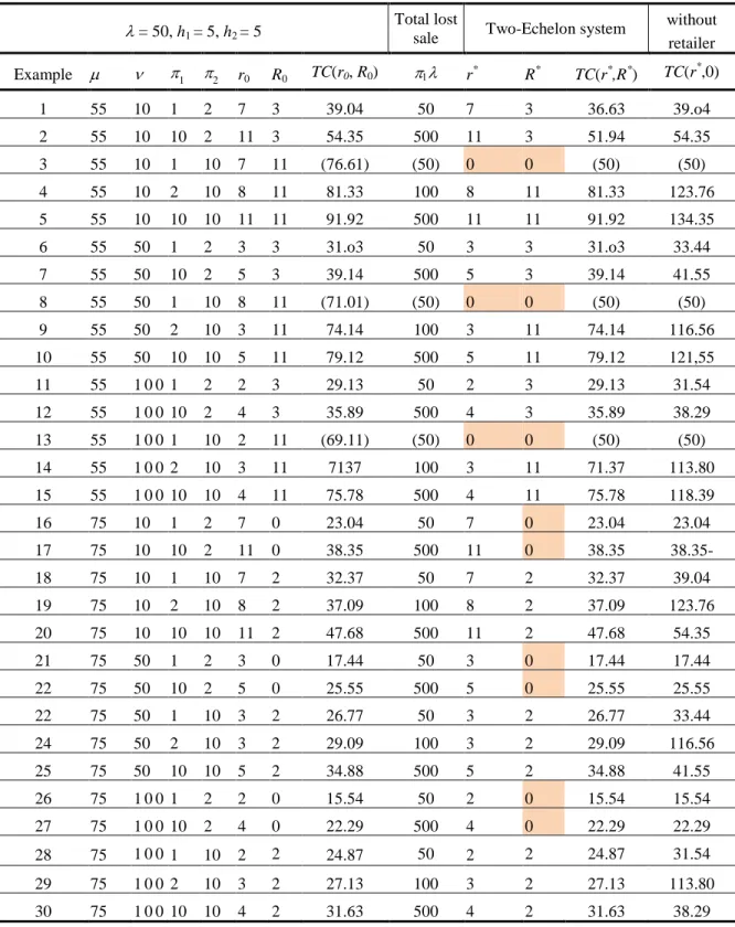
Table 1, we present 24 test examples which are different according to their service rates = 55, 75,

lead time rates  = 10, 50, 100, lost sale costs  = 1, 2, 10, and backordering costs  = 210. For all

examples  = 50 and h1 = h2 = 50.

In rows 3, 8 and 13 C1 (r0)  but TC (r0, R0) = C1 (r0) C2 (R0) = 50Thus, for these

examples the minimum total cost occurs when retailer supplies all his demands from another source (i.e., “total lost sale” and r*  0, R* 0), and therefore no inventory system for both retailer and supplier is needed.

Optimal policies for other examples reveal that parameters of the optimal inventory policy of supplier and retailer do not depend on each other, thus those optimal policies can be derived separately. The last column shows the total system cost when the retailer is omitted from the system, and the column before the last column shows the optimal total cost for the case of two echelon system. Column 9 shows the case of total lost sale Note that in most examples the optimal total cost of two-echelon system is less than the one for without the retailer system.

5. CONCLUSIONS

In this paper, we proposed a two echelon supply chain where supplier is a service system with an attached inventory and both supplier and retailer follow base stock inventory policy. We assumed that the arrival of customers to the retailer forms a Poisson process and the demands which arrive during the time that the supplier has no on-hand inventory are lost to the supplier and retailer buys product from another source with zero lead time and additional cost. Service time and replenishment lead time

of supplier’s system are exponentially distributed. We derived stationary distribution of joint queue length and on-hand inventory of the supplier.

Table 1 Optimal policy and optimal total cost of test examples. = 50, h1 = 5, h2 = 5

 _{Total lost}

sale Two-Echelon system

without retailer Example   ₁ ₂ r0 R0 TC(r0,R0)  r* R* TC(r*,R*) TC(r*,0)

1 55 10 1 2 7 3 39.04 50 7 3 36.63 39.o4

2 55 10 10 2 11 3 54.35 500 11 3 51.94 54.35

3 55 10 1 10 7 11 (76.61) (50) 0 0 (50) (50)

4 55 10 2 10 8 11 81.33 100 8 11 81.33 123.76

5 55 10 10 10 11 11 91.92 500 11 11 91.92 134.35

6 55 50 1 2 3 3 31.o3 50 3 3 31.o3 33.44

7 55 50 10 2 5 3 39.14 500 5 3 39.14 41.55

8 55 50 1 10 8 11 (71.01) (50) 0 0 (50) (50)

9 55 50 2 10 3 11 74.14 100 3 11 74.14 116.56

10 55 50 10 10 5 11 79.12 500 5 11 79.12 121,55

11 55 1 0 0 1 2 2 3 29.13 50 2 3 29.13 31.54

12 55 1 0 0 10 2 4 3 35.89 500 4 3 35.89 38.29

13 55 1 0 0 1 10 2 11 (69.11) (50) 0 0 (50) (50)

14 55 1 0 0 2 10 3 11 7137 100 3 11 71.37 113.80

15 55 1 0 0 10 10 4 11 75.78 500 4 11 75.78 118.39

16 75 10 1 2 7 0 23.04 50 7 0 23.04 23.04

17 75 10 10 2 11 0 38.35 500 11 0 38.35 38.35-

18 75 10 1 10 7 2 32.37 50 7 2 32.37 39.04

19 75 10 2 10 8 2 37.09 100 8 2 37.09 123.76

20 75 10 10 10 11 2 47.68 500 11 2 47.68 54.35

21 75 50 1 2 3 0 17.44 50 3 0 17.44 17.44

22 75 50 10 2 5 0 25.55 500 5 0 25.55 25.55

22 75 50 1 10 3 2 26.77 50 3 2 26.77 33.44

24 75 50 2 10 3 2 29.09 100 3 2 29.09 116.56

25 75 50 10 10 5 2 34.88 500 5 2 34.88 41.55

26 75 1 0 0 1 2 2 0 15.54 50 2 0 15.54 15.54

27 75 1 0 0 10 2 4 0 22.29 500 4 0 22.29 22.29

28 75 1 0 0 1 10 2 2 24.87 50 2 2 24.87 31.54

29 75 1 0 0 2 10 3 2 27.13 100 3 2 27.13 113.80

The key result is that stationary distribution is of product form and the marginal steady state

distribution of queue length is equal to the steady state queue length distribution in the classical M /M/

1/ ∞ and the marginal steady state distribution of on hand inventory of the supplier is equal to the steady state queue length distribution in the classical M /M /r /r.. The resulting distribution was employed to compute the performance measures of the systems. We showed when the inventory position of supplier is non-zero the total cost is convex. We obtained the optimal policy and its related optimal total cost. Optimal inventory policy and its related optimal total cost were investigated via several numerical examples. From numerical results it was shown that in most examples the optimal total costs of two-echelon inventory system (addition of the retailer) is much lower than the one for without the retailer system.

ACKNOWLEDGEMENT

We are grateful to Dr. Babak Ghalebsaz Jeddi for the stimulating discussions and his helpful comments.

REFERENCES

[1] Berman O., Kim E. (2001), Dynamic order replenishment policy in internet-based supply chains; Math Meth Oper Res 53; 371–390.

[2] Berman O., Sapna K.P. (2002), Optimal service rates of a service facility with perishable inventory items; Naval Res Logist 49; 464–482.

[3] Berman O., Kim E. (2004), Dynamic inventory strategies for profit maximization in a service facility with stochastic service, demand and lead time; Math Meth Oper Res 60; 497–521.

[4] Haji R., Saffari M., Haji A. (2011), Inventory and Service System in a Two-Echelon Supply Chain Using Base Stock Policy; Proceedings of 22nd POMS Annual Conference; Reno, Nevada, USA, Paper number 020-0324.

[5] He Q.M., Jewkes E.M., Buzacott J. (2002), Optimal and near-optimal inventory policies for a make to order inventory-production system; European Journal of Operational Research 141; 113-132.

[6] Jagers A.A., Van Doorn E.A. (1986), On the continued Erlang’s loss function; Operations Research Letters 5(1); 43-46.

[7] Saffari M., Haji R., Hassanzadeh F. (2011), A queueing system with inventory and mixed exponentially distributed lead times; Int J Adv Manuf Technol 53; 1231-1237.

[8] Saffari M., Haji R. (2009), Queueing system with inventory for two-echelon supply chain; CIE International Conference, 835–838.

[9] Schwarz M., Daduna H. (2006), Queueing systems with inventory management with random lead times and with backordering; Math Meth Oper Res 64; 383–414.

[10] Schwarz M., Sauer C., Daduna H., Kulik R., Szekli R. (2006), M/M/1 Queueing systems with inventory; Queueing Syst 54; 55–78.

[11] Sigman K., Simchi-Levi D. (1992), Light traffic heuristic for an M/G/1 queue with limited inventory; Ann Oper Res 40; 371–380.