Ranvir S. Dhaliwal
Comparison of Tissue Excitation and Mechanical Property Derivation Methods in VisR Ultrasound
Introduction
Soft tissue refers to a wide range of biological matter that “binds, supports, and protects our human body and structures such as organs” [1]. This includes fats, muscles, tendons, ligaments, synovial tissue, blood vessels, lymph vessels, and peripheral nerves [2]. The mechanical
properties of soft tissue vary throughout the body [1]. For example, the elastic moduli of soft tissue can vary as much as four orders of magnitude [3]. Quantitative examples of mechanical properties of soft tissue are a bulk modulus of 0.48 for stomach, 0.28 for liver, 0.49-0.25 for heart, and 0.15 for lung and tangent shear moduli of 8-45, 37-340, 60-148, and 10-54 for stomach, liver, heart, and lung tissues respectively [4]. The Poisson’s ratio of soft tissue generally ranges from 0.49 to 0.499 meaning it is almost incompressible [3]. Soft tissue is generally anisotropic and responds nonlinearly to tensile stress [1]. Proteoglycans form a common amorphous matrix that many soft tissue fibers are embedded in and may contribute to the viscoelastic properties of soft tissue [5]
Abnormalities in soft tissue are often indicative of medical disorders. Some of these
abnormalities include tumors and arterial hardening from atherosclerosis [6]. Ultrasound is one medical imaging device used for identification of soft tissue abnormalities. Some advantages of ultrasound in medical imaging over other techniques such as MRI include an ability to produce real-time images in 2D, low cost, non-invasiveness in most cases, portability, and safety since the frequencies used for imaging are not known to cause tissue damage and no ionizing radiation is involved. Commercial medical ultrasound systems also offer a spatial resolution approaching that of magnetic resonance microscopes. Limitations of medical ultrasound include its general inability to image bone or gas, the tradeoff between spatial resolution and depth, and the need for a skilled operator with anatomical and ultrasound knowledge for optimal resolution [7]. Despite its benefits, conventional ultrasound along with many other imaging techniques is sometimes inadequate in detecting the changes in mechanical properties of tissue. In [3], it is stated that “during many abdominal operations, palpation is used to assess organs, such as the liver, and it is not uncommon for surgeons at the time of laparotomy to palpate tumors that were undetected preoperatively by CT, magnetic resonance (MR), or ultrasound.” Changes in mechanical
properties of tissue can result from a variety of diseases including fluid collection in intracellular spaces, or as is the case in cancer, loss of lymphatic systems [3]. While palpation has been used for centuries in gathering qualitative data about the mechanical characteristics of tissue, more quantitative techniques exist.
quantitative results. This technique offers an advantage over techniques that manually palpate the surface of the skin because ARFI allows direct excitation of the region of interest and avoids surrounding interference [3]. Some concerns with using ARFI include tissue heating and cavitation. Heating is the result of an energy transfer from the acoustic wave to the tissue and cavitation is the production of cavities within the tissue. The higher intensity of ARFI pulses compared with B-mode imaging increases the concern for heating. Still, the short duration and low repetition frequency of pulses means the danger of overheating or cavitation are low [6]. Elastic modulus has been the standard mechanical property measured in ARFI [9] and is probably the closest to what is felt with palpation [3]. However, biological materials are
viscoelastic [10]. There are two directions to go with for determining the viscosity and elasticity of biological tissue: either through shear wave or displacement measurements [11]. A shear wave occurs when a layer of elastic, solid material is subjected to a force on two opposite faces, with each force in an opposite direction [12]. The particles in the wave will oscillate transverse to the direction of wave propagation. Shear waves are often the result of compression waves in which wave propagation and particle motion are aligned [13]. Qualitatively, higher shear wave speeds and smaller displacements reflect a higher elasticity. By tracking the shear wave propagation outside the region of excitation the shear modulus can be estimated [11]. Since tissue generally has a Poisson’s ratio ranging from 0.49 to 0.499, it is incompressible. This means that elastic modulus is one third the size of shear modulus [3]. The drawback of measuring shear wave is that it assumes the tissue being studied is homogeneous even outside the region of excitation. Methods that study directly the region of excitation involve measuring the displacement in the ROE and fitting to appropriate viscoelastic models. There are three such methods: KAVE, MSSER, and VisR. The first two techniques involve numerous repeated pushes until steady state displacement is achieved. With KAVE, the displacement is fitted to viscoelastic models [9] and with MSSER, tissue creep and recovery are observed and parameters such as relaxation time are calculated. A drawback with both aforementioned techniques is they require many pushes to achieve steady state displacement which could result in undesired bio effects as well as requiring a high framerate, time duration, and energy expenditure [9]. VisR is a third method of measuring mechanical properties by fitting displacement to the MSD model [14].
The following figure shows the MSD model as a spring and dashpot in parallel with a mass at the end.
The spring accounts for elasticity and the dashpot for viscosity. Since the two components are in parallel, the displacement and velocities of the spring and dashpot are equal. The displacement of the spring is proportional to the force applied with the constant of proportionality called
elasticity. The force in the dashpot is proportional to its rate of displacement with a constant of proportionality called viscosity [16]. The total force applied to a body represented by a MSD model is the sum of the forces in the spring, dashpot, and mass.
Fspring(t)=Ex(t), (1)
Fdashpot(t)=μdx dt (2) F(t)=Fspring(t)+Fdashpot(t)+ma=Ex(t)+μdx
dt + md2u
d t2 (3) [17]
F is force, m is mass, E is elasticity, µ is viscosity, and x is displacement.
To solve for displacement in VisR, the ARFI excitation (F(t) in equation 3) is modeled as a rectangular wave. It should be noted that in reality an ARFI excitation is not a perfectly
rectangular waveform because it takes time to build up and die down. By denoting the amplitude of excitation as A, duration of excitation as tARF, and the time separation between multiple
excitations as ts, equation (3) can be rewritten for VisR as:
x(t)+ω2τ μdx dt +ω
2md2u
d t2 =S ω
2 ¿
(if2excitations used)
Where ω=
√
Em, τ= μ E, S=
A μ .
τ is the ratio of viscosity and elasticity. Thus, a higher τ value indicates smaller elasticity, greater viscosity, or both. Based on equations (1) and (2), the physical significance of higher elasticity is smaller displacement and higher viscosity means slower displacement and recovery rates. This is illustrated in figure 2.
time (s) 10-3
0 0.5 1 1.5 2 2.5 3
d is p la ce m e n t ( u m ) 0 1 2 3 4 5 6
7 Effect of Elasticity and Viscosity on Displacement
Figure 2. Focal displacement from 3 ARFI excitations of Confor Foam with varying elasticity and viscosity. Displacement magnitude is seen to correlate negatively with elasticity and viscosity.
The blue, green, and red materials (meaning material’s whose displacement profiles in Figure 2 are these colors) were subjected to the same magnitude, duration, and spacing of ARFI
excitations. The green material has the same elasticity as the blue material but is has a higher viscosity. Consequently, its rate of displacement during the three excitations is much slower and as a result its magnitude of displacement is also smaller than the blue material’s. The recovery after excitations is also more gradual for the green material. The red material has much higher elasticity than the blue material while keeping the same viscosity. This causes the red material to displace less than the blue material.
VisR estimates s, Ω, and τ by fitting the displacement of the unknown material to equation (4) using nonlinear least squares minimization [14]. In practice, the attenuation of the tissue that is excited is unknown; therefore, the exact force at the focus is unknown so viscosity and elasticity cannot be solved for. The advantages of VisR are that it requires only a few excitations and can still solve for the relaxation time constant τ without knowledge of the force amplitude
experienced within the material at the focus.
Farther investigation that compares the accuracy of results using 1, 2 or 3 pushes is needed. Existing research shows that 1 and 2 pushes produce similar results at the focus but 2 pushes produces valid readings for a larger region around the focus. Overall, VisR has been shown to produce results consistent with MSSER but with increased efficiency. A drawback of VisR is that it does not consider inertia from surrounding tissue encompassed within the ARFI excitation. This could produce significant error for large focal configurations or higher density materials [9]. The underlying purpose of this research is to compare the accuracy and precision of the τ value of a nonlinear material generated using various iterations of VisR or an alternative look up table approach which will be explained shortly. A nonlinear material is used because soft tissue behaves nonlinearly. Even though by definition a nonlinear material will not have constant mechanical parameters, VisR is still used to produce clinically relevant measurements by estimating these parameters by modeling a nonlinear material as linear.
The look up table is an alternative method to VisR for determining viscosity. Just like VisR, it involves exciting a tissue using 1, 2, or 3 pushes. Excitations are simulated on multiple nonlinear materials with known parameters. Unlike VisR, the displacement profiles of these excitations are not fit to a MSD model; rather, they are used to generate a reference table. The properties of an unknown material is estimated as equivalent to the properties of the simulated material in the look up table whose displacement profile most closely matches the displacement profile of the unknown material. The lookup table allows for solving of elasticity, viscosity, and τ.
It is hypothesized that the lookup table will produce more accurate results because it compares displacements which means error will be present in both materials being compared and will thus not affect the comparison. Additionally, the lookup table estimates the unknown material
fitting the MSD model to the displacement profile of an unknown material and is thus more susceptible to error. It is also hypothesized that number of pushes will have no effect on the lookup table because, once again, it depends on a comparison while VisR will also not be affected by number of pushes based on results from earlier studies on a linear material. Methods
Two methods of simulating tissue response to excitation are used: finite element method and ultratrack.
Finite Element Method
The finite element method is used to simulate the displacement of nonlinear material in response to an applied load. This is done through the FEM solver called LS Dyna (Livermore Software Technology Corp., Livermore, CA, USA). Before running the simulation, the following criteria must be established.
First, a mesh for the nonlinear material is created. The simulated material is a cube of 11.7 cubic centimeters. To increase simulation speed quarter symmetry is used meaning only a quarter of the mesh is used in simulation and the results are mirrored across bisecting midlines. Thus the mesh dimensions are 0.975cm (x) by 1cm (y) by 3 cm (z). Spacing is .025cm between nodes in all directions making 40 nodes in the x, 41 in the y, and 121 in the z directions.
For ARFI excitations, a five element thick perfectly matched layer (PML) encompasses the nonlinear material in question. The purpose of the PML is to prevent any waves from rebounding off the boundary of the material. Because no nonlinear PML exists in Dyna, a linearly elastic PML was used and it was not always perfectly matched to the nonlinear material.
Additionally, the force magnitude and location are specified. This is done in two ways. The force can be entirely focused on a single node (the focus) in the mesh. This is referred to as a point load. Alternatively, the force is distributed across a volume of nodes with a different magnitude for each node. In this case, the force profile replicates that created by ultrasound. This is referred to as ARFI excitation and is a more realistic depiction of force distribution from ultrasound than a point load is.
Figure 3. ARFI Excitation Profile in 10kPa, 1 Pa*s Confor Foam Mesh (LS Dyna)
In Figure 3, the pml layer can be seen as the blue material around the outside boundary of the mesh and the white shading is where the force is applied.
The temporal spacing of excitations is also specified. Three push spaceings were experimented with before settling on the one with 0.3 milliseconds between pushes. The ultrasound excitation time profiles for 3 pushes are given in table 1.
Table 1. ARFI Excitation Profile across Time
Excitation (1 == On, 0 == Off)
0.3 ms separation
0 0
1 5.6e-6
1 5.2e-5
0 7.2e-5
0 3.72e-4
1 3.776e-4
1 4.24e-4
0 4.44e-4
0 7.44e-4
1 7.496e-4
1 7.96e-4
0 8.16e-4
0 0.003
Furthermore, the material being used must be specified. The material used in this work is listed in the Dyna Manual as Confor Foam and material number 62. The material is described as “a nonlinear elastic stiffness in parallel with a viscous damper”. The elasticity and viscosity of Confor foam change with time according to the following formulas
Viscosity:V2t=V2
(
|1−V|)
n2 Elasticity:E❑1t=E1(V−n1)
In the above formulas, V2 is initial viscosity, E1 is initial elasticity, V2t is viscosity at time step t,
E1t is elasticity at time step t, V is the ratio of the volume at time step t to the initial volume, and
n1 and n2 are measures of nonlinearity for elasticity and viscosity, respectively.
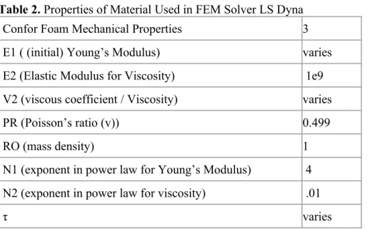
Confor Foam is chosen because of these nonlinear viscoelastic properties. Viscosity, elasticity and degree of nonlinearity as well as other mechanical properties can be changed by the user. The values used are listed in table 2.
Table 2. Properties of Material Used in FEM Solver LS Dyna
Confor Foam Mechanical Properties 3
E1 ( (initial) Young’s Modulus) varies
E2 (Elastic Modulus for Viscosity) 1e9
V2 (viscous coefficient / Viscosity) varies
PR (Poisson’s ratio (v)) 0.499
RO (mass density) 1
N1 (exponent in power law for Young’s Modulus) 4 N2 (exponent in power law for viscosity) .01
τ varies
E2, RO, and N1 are nonlinear properties of this material whose values are the ones
recommended for Confor foam in the Dyna manual. Poisson’s ratio is 0.499 to be accurately represent human soft tissue. N2 represents a degree of nonlinearity for viscosity. The manual recommended an N2 value of 0.2; however, ARFI excitations using both long (0.47
Figure 4. Point load excitations and VisR fits for 1, 2, and 3 Pushes 0.47ms apart on Confor Foam with N2 equal to 0.2. The focal displacement is oscillatory and unrealistic for soft tissue. To produce a displacement profile more consistent with human tissue, n2 was decreased from .2 to .01. This change is based on the following formula for the material’s viscosity which changes with time:
V2t=V2
(|
(1−V)|)
n2Where V is the ratio of current volume (at the time step) to initial volume. V should be close to 1 since the material is almost incompressible (as Poisson’s ratio is 0.499). By changing n2 to .01, there should be much less change in viscosity. This change produced a more realistic
displacement profile, so it was used for the rest of the experiment, and its data are presented and analyzed, unless otherwise specified. Figure 2 typifies the displacement profiles generated after making this change.
The different materials used for VisR and fitting to the lookup table as well as for generating the lookup table are all variations of the Confor Foam just described. The difference among the materials is in their elasticity (E1) and viscosity (V2) (and thus their τ).
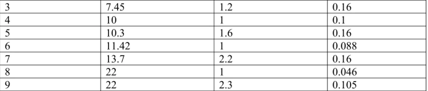
Test materials are those that are fit to VisR and the lookup table. Each test material undergoes sequences of 1, 2, and 3 pushes so the displacements from each sequence can be compared to the corresponding lookup table and fit to VisR. The true elasticity, viscosity, and τ values for each test material are given in table 3.
Table 3. Elasticity, Viscosity, and τ for Test Materials
Test Material Elasticity (kPa) Viscosity (Pa*s) τ (ms)
1 1 1 1
3 7.45 1.2 0.16
4 10 1 0.1
5 10.3 1.6 0.16
6 11.42 1 0.088
7 13.7 2.2 0.16
8 22 1 0.046
9 22 2.3 0.105
These test materials were selected to represent a broad spectrum of elasticities and viscosities ranging from 1kpa to 22kpa and 1 Pa*s to 3.5 Pa*s. Some of these values are also not within the bounds of the look up table and so test how well the lookup table fits to materials both inside and outside its range of material values.
For generating the look up table, elasticity is varied from 5kPa-15kPa, inclusive, at 1kPa intervals and for each elasticity the young’s viscosity is varied from 0.5 to 3 Pa*s by 0.5 Pa*s intervals. Thus there are 66 different materials in the look up table. The look up table is simply an array containing all of these displacement vectors. Thus, each look up table contains 6 rows for each viscosity, 11 “pages” for each elasticity, and 121 columns for displacement. There are three look up tables, one each for 1, 2, and 3 pushes. All lookup tables are normalized by dividing the displacement profile of each material by the max displacement of that material. Normalization is done because in real tissue, the magnitude of the excitation at the focus is unclear so a lookup table cannot be generated using the same exact force. Different forces on the same material may produce different displacement profiles. Normalization allows comparison of the shape of displacement profiles without regards to their magnitudes.
Ultratrack
Ultratrack takes the output from FEM and modifies the displacement to reflect the error
associated with tracking displacement using an ultrasound system. Error in ultrasound tracking of displacement comes from shearing or the uneven displacement of scatterers within the tracking point spread function. Averaging of displacement causes underestimation of displacement compared with FEM [19]. Another consequence of ultrasound tracking is the presence of jitter or increased displacement variance due to reduced echo signal correlation [20]. Ultratrack is performed through Matlab and python code that ultimately generates a new
displacement profile. Ten iterations (seeds) of ultratrack are performed on each test material. Each iteration produces a slightly different displacement profile because the location of scatterers is pseudorandom for each iteration. While in real tissue multiple excitations and trackings in the same position would produce the same image, the location of scatterers in a tissue is not known prior to imaging. Thus, running multiple iterations in simulation reflects multiple possibilities for scatterer locations. Each of these displacement profiles is modified by adding noise to achieve a 40 dB signal to noise ratio. VisR is conducted by fitting the MSD model to each of the 10 different noisy displacement profiles generated for each test material.
Figure 5. Displacement at focus of 3 push ARFI Excitation from FEM and after simulated ultrasonic tracking. Error from ultrasonic tracking causes underestimated and noisy displacement profiles when compared to the true FEM displacement profile. Different scatterer configurations also cause variation among simulated ultrasonically tracked displacement profiles.
All ultratrack generated displacements are smaller in magnitude (except towards the end of recovery) than the FEM displacement. This is due to shearing. Furthermore, the ultratrack seeds vary among themselves in terms of displacement magnitude although many have similar
magnitudes. This shows the effect of unknown scatterer positioning during imaging. Each seed also has 40 dB of signal to noise ratio which causes its displacement profile to contrast with the smooth profile from FEM (dotted line).
To create a lookup table using Ultratrack, the FEM focal displacement for each material in the lookup table must also undergo 10 iterations of ultratrack. Unlike the test materials, no noise is added to the ultratrack displacements for the lookup table. Instead, the average of the focal displacements from the 10 iterations for each material is used as the displacement data for that material in the lookup table. This is done to minimize error and produce the best possible
representation of the displacement tracked from ultrasound, regardless of scatterer configuration. The look up table is simply an array containing all of these displacement vectors.
To use the look up table, the displacement profile of each material in the look up table is individually compared with the normalized displacement profiles of all ten seeds (iterations) of each test material using code created in Matlab. Comparison is done using normalized cross correlation. The look up table material that has the highest cross correlation value, regardless of time lag, has its properties taken as the estimate for the test material seed’s properties.
Simulations were run on the KillDevil supercomputing cluster at UNC.
The only data analysis conducted on FEM data was to compare the effect of using a point load to using an ARFI excitation on the results from VisR. The rest of the data analysis used the test materials and lookup table materials whose displacement data had undergone ultratrack. The Wilcoxon rank sum test was used to test the validity of the null hypothesis that there is no difference between push numbers; specifically, there is no difference between 1 and 2, 1 and 3, and 2 and 3 pushes. This was done for the lookup table and VisR approaches, using τ for both as well as elasticity and viscosity for the former, and done for all test materials. The τ value from VisR was compared to the value from the lookup table for all materials by using box plots. Results
FEM VisR: Point load versus ARFI excitation
Table 4 shows the MSD fit to displacement induced by 1, 2, and 3 excitations from both ARFI and point loads with multiple excitations spaced 0.47 milliseconds apart. Displacement data used was generated from FEM but did not undergo ultratrack. The material’s elasticity is 10kpa, viscosity is 1 Pa*s and the τ value is 0.1 milliseconds. This is the only time a point load, or 0.47ms spacing, or pure FEM data (without ultratrack) is discussed in this study.
Table 4. τ value from VisR fit to ARFI and Point Loads with 0.47ms between Excitations τ (milliseconds)
ARF Pt
1 push 1.3 0.30245
2 push 1.3 0.29688
3 push 1.3 0.29633
The data shows no difference from varying the number of pushes. The τ value of the point load is closer to the true value of 0.1 milliseconds. The percent errors for ARFI and point load are 1200 and 200, respectively.
Lookup Table Approach versus VisR
Figure 6. τ values obtained from VisR and Lookup Table approaches.
Figure 7. τ values obtained from VisR and Lookup Table approaches. Lookup table results show greater accuracy and precision.
In all cases, the lookup table is more accurate than VisR. Additionally, there is less variance among the results for 1, 2, and 3 pushes using the lookup table. For the two 1kPa materials, all lookup table results for each material were identical across seeds and number of pushes. Thus, no plot is visible for these two cases.
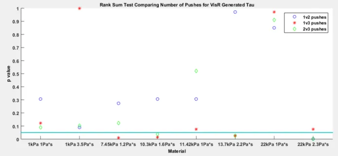
Figure 8 shows the results of a Wilcoxon rank sum test comparing elasticity, τ, and viscosity estimates for each material from VisR using 1 and 2, 1 and 3, and 2 and 3 pushes. The blue line shows the alpha value of 0.05.
Figure 8. P value of Wilcoxon Rank Sum Test comparing push numbers for VisR. Some
statistically significant difference is present among push numbers for some materials. There is no discernible pattern to the error.
Figure 8 shows a statistically significant difference exists between using 1 and 3 pushes for the 7.45 kPa, 1.2 Pa*s; 10.3 kPa, 1.6 Pa*s; and the 13.7 kPa, 2.2 Pa*s materials and between using 2 and 3 pushes for the 10.3kPa, 1.6 Pa*s; 13.7 kPa, 2.2 Pa*s; and 22kPa, 2.3 Pa*s materials.
1v2v3 Pushes for Lookup table
Figure 9. P value of Wilcoxon Rank Sum Test comparing push numbers for Lookup Table. There is no statistically significant difference between using 1, 2, or 3 pushes for the lookup table.
Since the results across pushes for each 1kPa material were identical, their results were omitted. With all p values greater than the alpha value of 0.05, there is no statistically significant
difference between using 1, 2, and 3 pushes for the lookup table approach. Lookup Table Error
Figure 10. Error in viscosity and elasticity estimates using Lookup Table. Error is generally greatest when the elasticity of a material is outside the range of the lookup table.
The elasticity error has a pretty constant median value and spread for the materials within the lookup table range of 5kPa to 15kPa. The 1kpa materials and 22kpa materials are all outside the lookup table range and they have higher elasticity error with a tight spread of errors. The
viscosity range of the lookup table is 0.5 Pa*s to 3 Pa*s. Only the 1kPa 3.5 Pa*s has a viscosity outside this range but its viscosity error is not significantly greater or less than any other
material’s error. Overall, error in viscosity shows greater variance for each material than their error in elasticity. The highest viscosity error is with two of the materials that have an elasticity out of the LUT (lookup table) bounds: 1kpa 1Pa*s and 22kPa 2.3 Pa*s materials.
Discussion
The results in table 4 show that the true τ value of a material is not reflected when fitting VisR to an ARFI excitation induced displacement, even before introducing the error associated with ultrasonic tracking. An explanation for this phenomenon is inertia which is the mass-dependent tendency of an object to resist a change in motion [21]. Since an ARFI excitation causes a displacement in a volume of material extending beyond the focal point, inertia is present and acts to prolong the material’s displacement and recovery causing the τ value to artificially increase [14]. This explanation is supported by the results in table 4 of fitting VisR to FEM generated displacement from a point load on the same material. Although the error is 200% for the point load case, this is much lower in comparison to the ARFI excitation. The point load excites only at the focus and thus prevents error from inertia from surrounding tissue. Previous studies have shown VisR on point load in a linear material to have almost no error [14]. The 200% error on the point load in this experiment may be due to slight changes in the material’s viscosity or elasticity due to nonlinearity. While using a point load makes VisR more accurate, unfortunately, the point load is only possible in FEM.
The over 1000% error from inertia when using VisR makes an alternative method desirable. Figures 6 and 7 show the lookup table as a promising alternative. The lookup table circumvents the error associated with inertia and shearing because this error is present in both materials being compared and thus does not affect the comparison. Once the best fit is found, the estimation of the unknown material’s properties are made from the best fit material’s known properties which are also independent of inertia or shearing. This also explains why variation in results from using different push numbers is eliminated in the lookup table. The small amount of variation present in the results using the lookup table is likely due to variations in scatterer locations which caused different displacements for each seed. Although most of these displacements are similar there are also some outliers which may have been incorrectly fitted. Additionally, the lookup table is limited by the range of materials it contains and the fineness of its elasticity and viscosity sampling intervals.
degree of error associated with the time of excitation that must be measured and the lookup table can then be generated using this timing. Wave reflections are also an issue. In ls-dyna, a
perfectly matched layer (pml) can be placed on the boundary of the material to rapidly attenuate any waves that reach it. Unfortunately, no nonlinear pml materials exist and the elasticity of some of the pml layers used was different than the material they surrounded. These conditions are suboptimal and should be corrected in the future. Finally, anisotropy is a factor not yet considered. An anisotropic material has different properties in different directions [22]. While anisotropy was not included in and does not affect these simulations, real soft tissue can be anisotropic. If an anisotropic material is compared to this lookup table, it may produce different results depending on the direction in which the excitation and imaging is conducted.
Figures 6 and 7 show that in the case of all the test materials, fitting the ultratrack generated focal displacements to the lookup table produced far more accurate results than fitting to VisR. Unlike the lookup table fits, the VisR fits show variation among push numbers in the τ value generated for a few cases. There is no trend in the material’s viscosity or elasticity or push numbers among these cases. More investigation is needed to identify the cause of this
inconsistent, occasional difference among pushes when using VisR. If this is due to variations in the displacement profiles among seeds then a larger sample may eliminate this difference.
The trends in figure 10 show that error using the lookup table approach is greater when the material’s elasticity is out of the range of the lookup table. In this case, the unknown material is fit to the boundary of the lookup table. This also explains why there is little variation in the estimates for these materials. The farther the unknown material’s elasticity is from the boundary, then the greater the error. Interestingly, two of the four materials with elasticity out of the LUT also had the highest error in viscosity. The viscosity of a material being out of the bounds of the lookup table did not have much of an effect on viscosity error. Since this was the case only for one material, however, no conclusions can be made on the effect on accuracy from viscosity being out of the LUT bounds.
Conclusion
Error associated with VisR estimates for τ (ratio of elasticity to viscosity) are over 1000%. Inertia is probably responsible for this error and it comes from the volume of tissue surrounding the focus that is excited when conducting ARFI. The error is not seen with a point load where only the focus is excited. However, a point load is only possible in simulation. The lookup table produces accurate τ, viscosity, and elasticity estimates and shows little difference between 1, 2, and 3 pushes. Limitations of the lookup table include the amount of materials it contains, the fineness of its elasticity intervals, imprecise force timings in real ultrasound that are not
Sources
[1] Holzapfel, G. A. (2000). Biomechanics of soft tissue No. 7
[2] Anatomy and physiology of soft tissue http://www.cancer.ca/en/cancer-information/cancer-type/soft-tissue-sarcoma/soft-tissue-sarcoma/the-soft-tissues-of-the-body/?region=sk. Ret rieved 4/3, 2017, from http://www.cancer.ca/en/cancer-information/cancer-type/soft-tissue-sarcoma/soft-tissue-sarcoma/the-soft-tissues-of-the-body/?region=sk
[3] Fatemi, M., Greenleaf, J. F., & Insana, M. (2003). Selected methods for imaging elastic properties of biological tissues. Annual Review of Biomedical Engineering, 5, 57-58-78. [4] Saraf, H., Ramesh, K. T., Lennon, A. M., Merkle, A. C., & Roberts, J. C. (2007). Mechanical
properties of soft human tissues under dynamic loading. Journal of Biomechanics, 40(9), 1960-1967. doi:http://dx.doi.org/10.1016/j.jbiomech.2006.09.021
[5] R. J. Minns, P. D. Soden, and D. S. Jackson. The role of the fibrous components and ground substance in the mechanical properties of biological tissues: A preliminary investigation. J. Biomech., 6:153–165, 1973.
[6] Iyo, A. Y. (2009). Acoustic radiation force impulse imaging: A literature review. Journal of Diagnostic Medical Sonography, 25(4), 204-205-211.
[7] Cootney, R. W. (2001). Ultrasound imaging: Principles and applications in rodent research. ILAR Journal, 42(3), 233-247. doi:10.1093/ilar.42.3.233
[8] Nightingale, K. R., & Palmeri, M. L. (2008). Acoustic radiation force impulse (ARFI) imaging: Fundamental concepts and image formation. In M. Fatim, & A. Al-Jumaily (Eds.), Biomedical applications of vibration and acoustics in imaging and
characterizations ()
[9] M. R. Selzo, & C. M. Gallippi. (2013). Viscoelastic response (VisR) imaging for assessment of viscoelasticity in voigt materials. IEEE Transactions on Ultrasonics, Ferroelectrics, and Frequency Control, 60(12), 2488-2500. doi:10.1109/TUFFC.2013.2848
[10] Pal, S. (2013). Mechanical properties of biological materials. Design of artificial human joints and organs (pp. 23-24-40)
[11] Nightingale, K. (2011). Acoustic radiation force impulse (ARFI) imaging: A review. Current Medical Imaging Reviews, 7(4), 328-329-339.
[12] Shear wave. (2015). Retrieved 12/15, 2016, from https://www.britannica.com/science/shear-wave
[13] Wave propagation. Retrieved 12/15, 2016,
from https://www.nde-ed.org/EducationResources/CommunityCollege/Ultrasonics/ Physics/wavepropagation.htm
One-Dimensional Mass-Spring-Damper Model," in IEEE Transactions on Ultrasonics, Ferroelectrics, and Frequency Control, vol. 63, no. 9, pp. 1276-1287, Sept. 2016. doi: 10.1109/TUFFC.2016.2539323
[15] Aparicio, J. (2013). Simmechanics: Simulating floor interaction/collision. Retrieved 3/27, 2017, from http://
embeddedprogrammer.blogspot.com/2013/01/simmechanics-simulating-floor.html
[16] Constitutive equations: Viscoelasticity. Retrieved 12/15, 2016, from http://www.umich.edu/ ~bme332/ch7consteqviscoelasticity/bme332consteqviscoelasticity.htm
[17] Walker, W. F., Fernandez, F. J., & Negron, L. A. (2000). A method of imaging viscoelastic parameters with acoustic radiation force. Physics in Medicine and Biology, 45, 1437-1438-1447.
[18] J. A. Jensen and N. B. Svendsen. “Calculation of pressure fields from arbitrarily shaped, apodized, and excited ultrasound transducers”. IEEE Trans. Ultrason., Ferroelectr., Freq. Control, vol. 39, no. 2, pp. 262-267, Mar., 1992
[19] Czernuszewicz, T. J., Streeter, J. E., Dayton, P. A., & Gallippi, C. M. (2013). Experimental validation of displacement underestimation in ARFI ultrasound. Ultrasonic
Imaging, 35(3), 196-213. doi:10.1177/0161734613493262
[20] M. L. Palmeri, S. A. McAleavey, G. E. Trahey and K. R. Nightingale, "Ultrasonic tracking of acoustic radiation force-induced displacements in homogeneous media," in IEEE Transactions on Ultrasonics, Ferroelectrics, and Frequency Control, vol. 53, no. 7, pp. 1300-1313, July 2006. doi: 10.1109/TUFFC.2006.1665078
[21] Inertia and mass. Retrieved 3/27, 2017,
from http://www.physicsclassroom.com/class/newtlaws/Lesson-1/Inertia-and-Mass [22] Anisotropic. Retrieved 3/27, 2017,
![Figure 1. Mass Spring Damper (MSD) model. [15]](https://thumb-us.123doks.com/thumbv2/123dok_us/8331617.2210347/2.918.109.533.805.1030/figure-mass-spring-damper-msd-model.webp)