HETEROTROPHIC EXTRACELLULAR ENZYMATIC ACTIVITY ACROSS GEOSPATIAL REGIMES IN THE ATLANTIC OCEAN
Adrienne Hoarfrost
A thesis submitted to the faculty at the University of North Carolina at Chapel Hill in partial fulfillment of the requirements for the degree of Master of Science in the Department of Marine
Sciences in the College of Arts and Sciences.
Chapel Hill 2015
Approved by:
Carol Arnosti
ABSTRACT
Adrienne Hoarfrost: Heterotrophic Extracellular Enzymatic Activity Across Geospatial Regimes in the Atlantic Ocean
(Under the direction of Carol Arnosti)
Heterotrophic activity in the marine water column plays a crucial role in the carbon cycle, affecting the amount of particulate carbon available to higher trophic levels, the amount of organic carbon preserved over geological timescales, and the balance of CO2 between the oceans and the atmosphere. Extracellular enzymes initiate the breakdown of organic matter, hydrolyzing it into sizes small enough to transport into the cell. The variability of heterotrophic extracellular enzymatic activity across geospatial regimes in the ocean may have an important impact on global carbon flux, yet the patterns of hydrolysis across latitude and depth, and the factors driving these patterns, remain poorly understood. This project investigates the
ACKNOWLEDGEMENTS
TABLE OF CONTENTS
LIST OF FIGURES ... VII
LIST OF TABLES ... VIII
INTRODUCTION ... 1
METHODS ... 5 Site Description and General Patterns of Circulation ... 5
Deep Water Circulation ... 6
Experimental Methods ... 14
Seawater collection ... 14
α-glucosidase and leucine aminopeptidase incubations and activity measurements ... 14
Polysaccharide substrate incubations and activity measurements ... 16
Seawater sampling for molecular analyses ... 17
DOC and Total Nitrogen sampling and analysis ... 18
Statistical Analysis Techniques ... 18
Polysaccharide Hydrolytic Diversity Using Shannon Diversity Indices ... 18
Compositional Dissimilarity Among Sampling Sites Using a Bray-Curtis
Dissimilarity Matrix ... 19
Multiple Regression Statistical Analysis of Environmental Parameters vs.
Hydrolytic Activity ... 20
RESULTS ... 21 Polysaccharide-Hydrolyzing Enzyme Activities ... 21
Influence of Environmental Parameters on Hydrolytic Activities ... 26
Enzymatic Hydrolysis of Monomeric Substrates ... 32
Patterns in Leucine Aminopeptidase Activities with Depth, Latitude, and Time ... 32
Patterns in α-glucosidase Activities with Depth, Latitude, and Time ... 35
DISCUSSION ... 38
APPENDIX A: DEPTH AND PHYSICOCHEMICAL CONDITIONS OF EACH SAMPLING SITE ... 49
APPENDIX B: STRATIFICATION ACROSS STATIONS SAMPLED IN THE SOUTH ATLANTIC ... 51
APPENDIX C: TOTAL ACTIVITY IS HIGHEST WHERE SHANNON HYDROLYTIC DIVERSITY IS HIGHEST ... 52
APPENDIX D: LINEAR RELATIONSHIPS OF INDIVIDUAL SUBSTRATES WITH ENVIRONMENTAL PARAMETERS ... 53
APPENDIX E: PERMUTATIONS OF ANOVA BEST FIT MULTIPLE REGRESSION MODELS ... 55
APPENDIX F: STRATIFICATION IMPACTS RATE OF DECREASE OF HYDROLYSIS RATE BELOW THE DCM ... 56
APPENDIX G: CURRENTS AND WATER MASSES OF THE ANTARCTIC REGION ... 57
LIST OF FIGURES
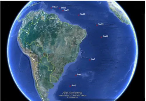
Figure 1 – Map of stations sampled during 2013 cruise KN210-04 to the South Atlantic ... 6
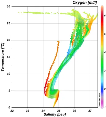
Figure 2 – T-S plot along the entire KN210-04 cruise track. ... 7
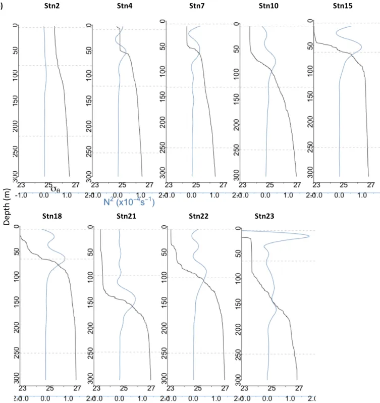
Figure 3 – A vertical transect of physicochemical parameters measured along the cruise track. 9 Figure 4 – CTD casts and density/stratification profiles for all stations sampled. ... 11
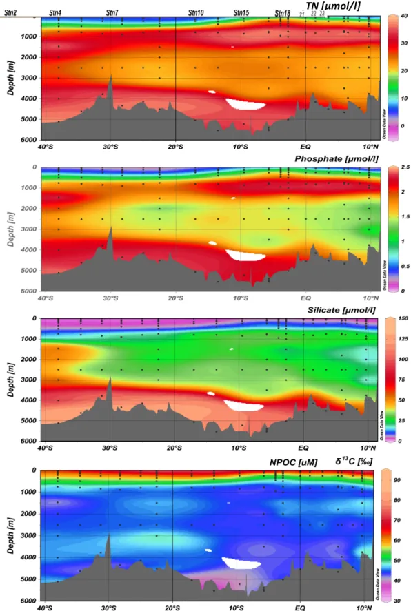
Figure 5 – A vertical transect of nutrients measured along the cruise track……….……..…..10
Figure 6 – Maximum polysaccharide hydrolysis rate at each site ... 22
Figure 7 – Summed polysaccharide hydrolysis activity by latitude and depth ... 23
Figure 8 – Shannon indeces (H) at each site ... 24
Figure 9 – Representative plot of enzymatic response time to polysaccharide substrate addition……….………...……26
Figure 10 – Aggregate polysaccharide hydrolysis rates vs. physicochemical parameters ... 27
Figure 11 – Best fit multiple linear regression model of hydrolysis rates and environmental variables ... 28
Figure 12 – Best fit multiple regression models for hydrolysis rates specific to individual substrates and environmental variables ... 30
Figure 13 – NMDS visualization of Bray-Curtis distances among enzyme activity assemblages in surface, DCM, and mesopelagic sampling depths at all stations, grouped by station ... 31
Figure 14 – NMDS visualization of Bray-Curtis distances among enzyme activity assemblages in surface, DCM, and mesopelagic sampling depths at all stations, grouped by depth ... 31
Figure 15 – Leucine aminopeptidase activity across stations for each depth ... 32
Figure 16 – Leucine aminopeptidase activity with depth for each station ... 33
Figure 17 – Representative trend of leucine aminopeptidase hydrolytic activity measured over the incubation time course ... 34
Figure 18 – α-glucosidase activity across stations for each depth ... 35
Figure 19 – α-glucosidase activity with depth for each station ... 36
LIST OF TABLES
Table 1 – Station numbers, latitude and longitude at stations sampled ... 6 Table 2 – Leucine aminopeptidase activity at T1 vs T3 at the six sites for which
INTRODUCTION
Heterotrophic breakdown of complex organic matter is an important component of the carbon cycle, operating in virtually every known habitat and impacting the flow of carbon on short and long timescales. In the marine water column, heterotrophic microbes play a
particularly important role in regulating the transformation and export of organic carbon. Heterotrophic microbes in the photic zone cycle approximately half of photosynthetically produced organic matter each year (Azam 1998), influencing the amount of particulate organic matter (POM) available to higher trophic levels or exported to deeper waters, as well as the equilibrium of CO2 between the atmosphere and oceans. The “microbial loop” in the epipelagic zone is especially crucial to the cycling of dissolved organic matter (DOM). Since DOM is too small for other trophic groups to access, the microbial loop is the only pathway by which DOM can be reincorporated into biomass (Azam & Malfatti 2007). Beyond the photic zone, microbial impacts on organic carbon degradation are still significant; just 1% of marine organic matter on average reaches the sediments after traveling through the deep ocean (Hedges & Keil 1995). Ultimately, an average of only 0.1% of the organic carbon produced by primary productivity in the surface ocean is preserved in sediments (Hedges & Keil 1995), so heterotrophic
remineralization of organic matter exerts a strong influence over the rate and extent of organic carbon preservation as well.
Understanding how complex organic matter is transformed and remineralized by marine heterotrophs, and how this activity varies geospatially, is thus vital to our understanding of the microbially-mediated carbon cycle on a global scale. Extracellular enzymes initiate the
which typically have a molecular size limit of ca. 600 Daltons (Weiss et al. 1991). Thus the first step of heterotrophic degradation of organic carbon is the extracellular hydrolysis of high-molecular-weight substrates into transportable sizes.
The accessibility of natural organic matter to marine heterotrophs is determined by the pool of extracellular enzymes available to hydrolyze it, and the substrate specificities of those enzymes. Extracellular enzyme availability ultimately depends on the cumulative enzymatic capacities of the microbial community, so extracellular enzymatic capacities of microbial communities in turn has a substantial impact on the heterotrophic carbon cycle. The functional capacities for extracellular enzymes may be distributed among different taxa within the
community (Martinez et al. 1996, Xing et al. 2014), such that no single group is capable of producing all the enzymes necessary to break down complex organic substrates. Instead, certain taxa may express particular enzymes that are able to partially break down substrates, while other taxa express different enzymes, such that microbial community dynamics as a whole results in a more complete breakdown of organic matter than any species in isolation is capable of (McCarren et al. 2010). Describing the variability in extracellular enzymatic activity in the marine environment, and understanding the factors that drive this activity, is therefore a fundamental step in our understanding of (and ability to predict) the global carbon cycle.
There is a gap, however, between the recognized importance of extracellular enzymatic activity in the global carbon cycle, and empirical measurements of activity in the environment. Most direct measurements of enzyme activity rely on monomeric substrate proxies (Hoppe 1983) that do not accurately represent the molecular size and complexity of natural organic matter (Warren 1996). Relatively few studies use macromolecular substrates (e.g. Obayashi & Suzuki 2005, Steen et al. 2012, Arnosti et al. 2012, Arnosti & Steen 2013). Considering both high- and low-molecular-weight substrates in the same study allows for comparison with results from previous studies while gaining unique insight into heterotrophic enzyme dynamics in the environment using substrates more representative of natural organic matter.
heterotrophic enzyme dynamics in the environment. Investigations of geospatial variations in enzyme activities are especially rare, particularly studies that measure enzyme activity in the deep ocean; in the open Atlantic Ocean, the focus of this study, only three studies have measured extracellular enzymatic activity in water below the epipelagic (Baltar et al. 2009; 2010; 2013), and these studies only measured hydrolysis of monomeric substrates. Only two studies have measured hydrolysis of macromolecular substrates with depth to date (Steen et al. 2012, D’Ambrosio et al. 2014), but these studies focused on marginal sea and coastal
environments. No studies have yet measured hydrolysis of macromolecular organic carbon in the deep open ocean.
Despite a need for better data coverage, patterns in the rate and diversity of hydrolysis of high-molecular-weight organic carbon are emerging. A cumulative look at a decade’s worth of data revealed global patterns in hydrolysis of high-molecular-weight substrates in surface seawater (Arnosti et al. 2011), with higher total hydrolysis rates and broader spectra of substrates hydrolyzed at lower latitudes than at higher latitudes. Hydrolysis patterns of most substrates were poorly correlated with temperature, and may instead mirror patterns in microbial biogeography, which exhibit higher species richness and diversity at lower latitudes (Fuhrman et al. 2008).
Microbial biogeography is a rapidly growing focus of research that is beginning to describe global patterns of microbial community diversity and richness (Martiny et al. 2006, Fuhrman et al. 2008, Zinger et al. 2011), resulting in initial attempts to model global
geospatial regions (Davey et al. 2001, DeLong et al. 2006, Shi et al. 2011) that will form the basis of further exploration and modeling.
Other potential factors that may be driving patterns of hydrolysis in the environment have been considered by other studies. Environmental factors are a major focus of these investigations, which have found that microbial communities (and relatedly, enzyme activity) are shaped more strongly by environmental distance than by geographic distance (Jiang et al. 2012), and that enzyme activities are more closely related to environmental parameters than community composition under some conditions (Kellogg & Deming 2014). Any thorough understanding of the functional stratification of heterotrophic communities and the factors that drive it will depend upon a better description of heterotrophic enzyme activities, including and especially extracellular hydrolytic enzymes, across geospatial regimes. Further, an
understanding of the factors that drive patterns of hydrolysis will be crucial to any accurate theory or predictive model of global enzyme dynamics, and ultimately of the global carbon cycle.
Within this framework, this project investigates hydrolysis of several high-molecular-weight organic substrates across a broad range of latitude and depth in the South and Equatorial Atlantic Ocean in order to better understand the geospatial variability in
heterotrophic extracellular enzymatic activities in the marine environment. Beyond describing the hydrolysis patterns of individual substrates, this project evaluates hydrolytic assemblages of substrates across multiple sites, enabling us to draw insights about the diversity of
substrates hydrolyzed with depth as well as the vertical and horizontal hydrolytic connectivity between sampling sites. In order to better understand the driving factors behind hydrolysis patterns, this project investigated the ability of ten environmental variables to predict
METHODS
Site Description and General Patterns of Circulation
Figure 1 – Map of stations sampled during 2013 cruise KN210-04 to the South and Equatorial Atlantic.
Station Latitude Longitude
Stn 2 38°S 45°W
Stn 4 31.25°S 41°W
Stn 7 22.5°S 33°W
Stn 10 9.5°S 26°W
Stn 15 2.7°S 28.5°W
Stn 18 3.5°N 39°W
Stn 21 6.5°N 48°W
Stn 22 8.25°N 50°W
Stn 23 9.75°N 55.3°W
Table 1 – Station numbers, latitude and longitude at stations sampled during 2013 cruise KN210-04.
Deep Water Circulation
Its associated Subantarctic Convergence Zone, directly outside the boundary of the ACC between 48 and 60
°
S, results in the formation of cold, low salinity AAIW where cold Antarctic surface water meets warmer South Atlantic surface water and sinks to intermediate depths typically between 700-900m. AAIW travels from south to north across the western SouthAtlantic and is detectable by its low salinity as far north as the Equator. Antarctic Bottom Water (AABW), formed by surface cooling on the Antarctic shelf, sinks and travels along the bottom of the Atlantic basin from south to north. It is detectable in deepest levels by a temperature minimum. Meanwhile, NADW is formed by deep convection in the Arctic Sea, and travels from north to south throughout the Atlantic, forming a large, distinctive wedge between ca. 1500-4000m in the South Atlantic. At the southernmost edge of the Atlantic basin, where NADW meets subantarctic waters, the NADW intersects with Circumpolar Deep Waters (CDW), and Upper and Lower CDWs are sometimes detectable above and below NADW (Appendix G). All of these water masses were observed along the KN210-04 cruise track (Figure 3, Figure 4).
Figure 2 – T-S plot with Salinity (S) on the horizontal axis and in situ Temperature (T) on the vertical axis. T
Station 2, the southernmost station at 38
°
S by 45°
W, was the location most notably characterized by CDWs at ca. 1500m and 3250m, observable by low oxygen relative to NADW (Figure 4). NADW was less prominent in the southernmost stations relative to the other more northern stations due to this influence of CDWs (Figure 4). AAIW, indicated by an oxygen maximum and salinity minimum, was quite prominent and was detected over a wide range of depths between ca. 500-1000m (Figure 3b). At equatorial stations 10, 15, 18, and 21-23, the oxygen maximum characteristic of AAIW was obscured by an oxygen minimum zone between ca. 75-1000m depth(Figure 3a). Antarctic Bottom Water was also detectable as a temperature minimum, most prominently at the deepest stations, Station 2 and Station 10 (Figure 3c).At Station 4 (31.25
°
S by 41°
W), NADW was much more distinct than at Station 2, detected over a greater range of depths from ~2000-3700m (Figure 4). AAIW was also quite distinct. The signature of CDW was still observable, indicated by an oxygen minimum between 1000-2000m, but unlike Station 2 only Upper Circumpolar Deep Water was detected (above the NADW), and Lower Circumpolar Deep Water was not detectable below the NADW. This was most likely due to the relatively shallow bottom at Station 4, which may have restricted flow of the deepest water masses at that location. Circumpolar Deep Water is less prominent but still detectable at Station 7 as an oxygen and temperature minimum between ~900-1300m, but is not detectable at Station 10.At more northern stations (Stations 10,15, 18, and 21-23), the AAIW became less
immediately above), but remained detectable only deeper at Stations 7-18 (~4000m), until it was no longer detectable at Stations 21-23, possibly due to shallower depths at Stations 21-23.
Figure 3 – A vertical transect of the cruise track, with contours of (a) oxygen (mL/L), (b) salinity (psu), (c) temperature
(°C), and (d) chlorophyll (ug/L) indicated by color. Each black or grey dot indicates a sampling point, while light gray vertical lines indicate stations where CTD data were used to anchor the contour plot.
4(a) Stn2
Stn4
Stn7
Stn10
Stn15
Stn18
Stn21
Stn22
Stn23
De
pth
(m
Figure 4 – CTD casts for all stations sampled. Each vertical section represents one station. (a) shows salinity (red),
oxygen (brown), potential temperature (blue), and chlorophyll (green). (b) shows potential density (black) and buoyancy frequency (light blue) in the upper 300m of the water column. Depths where samples were taken at that station indicated by horizontal dashed grey lines.
4(b) Stn2
Stn4
Stn7
Stn10
Stn15
Stn18
Stn21
Stn22
Stn23
De
pth
(m
Stratification in the upper water column varied from station to station as well (Figure 4b). In general, potential density profiles (in sigma-units, represented by σθ at each station) followed a similar trend, in which a surface mixed layer is underlain by a rapid increase in density with depth. This increase tapers to a more gradual increase with depth below. The vertical rate of change in density (i.e., the “stratification”) can be represented by the buoyancy frequency, N2. Although the magnitude of N2 varied by station, N2 was at a maximum within the
pycnocline (below the base of the mixed layer) for all stations, with the exception of Station 23 at which the Amazon River plume was present in surface waters. Station 2 was the least stratified, and generally the southernmost stations were less stratified than the northernmost stations (Appendix B, Figure 4b). Stratification at the pycnocline was highest at Station 15 and 18, where the OMZ was most prominent. At Station 23, stratification was highest at the salinity-driven density boundary between the fresh Amazon River plume at the surface and the high salinity water below. This was the highest N2 measured throughout the cruise. There was
another, smaller peak in N2 at ca. 125m where there was a second, temperature-driven
pycnocline.
Figure 5 – Nutrients measured from discrete samples along the cruise track of KN210-04. Each black dot indicates a discrete sample, from which a gridded contour plot was created along a vertical transect of the cruise track. a) Total Nitrogen (µM), b) Phosphate (µM), c) Silicate (silicic acid) (µM), and d) Dissolved Organic Carbon (or Non-Purgeable Organic Carbon) (µM) were measured.
Experimental Methods
Seawater collection
Seawater was collected at nine stations spanning latitudes from 38°S to 9°N (Figure 1, Table 1) – Stations 2, 4, 7, 10, 15, 18, 21, 22, and 23. Water was collected in Niskin bottles attached to a rosette equipped with a CTD and fluorescence detector. At each station, two liters of seawater was collected in two 1L Duran bottles from six different depths: surface, DCM, Mesopelagic, AAIW, NADW, and bottom water.
For each of the six depths sampled, two 1L glass Duran bottles were rinsed three times with seawater from the corresponding depth then filled to the one-liter mark directly from a single Niskin bottle, without using tubing. One of the two Duran bottles was allocated to DOC sampling and filtering for molecular biological samples, while the other was allocated to substrate incubations. Approximately 200mL of seawater from each incubation Duran bottle was sterilized in an autoclave(Wisconsin Aluminum Foundry 25X) for use as killed control incubations.
α-glucosidase and leucine aminopeptidase incubations and activity measurements
α-linked-glucose labeled with 4-methylumbelliferone (MUF; Chem Impex 21676) was added to one set of incubations, while leucine labeled with 4-methylcoumarinyl-7-amide (MCA; Sigma 62480-44-8) was added to another set. In both cases, the MUF or MCA tag fluoresces after it is cleaved from the substrate, and enzymatic activity is measured as an increase in
fluorescence over time. A change in fluorescence is then compared to a standard curve of known concentration of MUF or MCA, from which a hydrolysis rate is calculated.
For each substrate, triplicate samples of 4mL of seawater were incubated in plastic cuvettes at as close to in situ temperature as possible (Appendix A). Due to a limited number of incubators and temperature-stable locations aboard ship, available incubation temperatures were 3, 12, 15, 18, 25, and 28°C. A fourth incubation containing autoclaved seawater served as a kill control. A cuvette using 4mL autoclaved seawater with no substrate served as a killed blank, and a cuvette with 4mL live seawater and no substrate served as a live blank. Incubations were sampled at four timepoints, T0-T3. At each timepoint, 1mL from each incubation was added to 1mL of 0.2M borate buffer (pH 8) in a plastic cuvette and fluorescence emission was measured in a Turner Biosystems spectrophotometer (TBS-380). Later timepoints were determined based on the rate of activity at earlier timepoints – if activity was high (fluorescence went up sharply since the last timepoint), subsequent timepoints were taken sooner than if activity was low or zero. A typical timecourse for a rapidly-hydrolyzed substrate was 6hrs, 12hrs, and 24hrs; for a low- to no-hydrolysis substrate, 24, 48, and 72 hrs. No incubation was sampled later than 72hours. While specific time courses varied based on activity, all incubations for all substrates at all depths and stations were sampled at 24 hours to provide a common time point reference.
represent potential activities, but due to differences in timecourse α-glucosidase activities may represent a growth response whereas the shorter time course of leucine aminopeptidase likely does not.
Substrates were provided in saturating concentrations for all incubations. A saturation curve was necessary to ensure that the enzyme activity being measured was not a function of substrate concentration. The substrate concentrations used were determined by conducting a saturation curve over 24 hours. Since microbial enzymatic activity is typically highest in surface waters or close to the surface (Steen et al. 2012, Baltar et al. 2009), and leucine aminopeptidase activity is typically higher than α-glucosidase (Baltar et al. 2010; 2013), saturation
concentrations for leucine-MCA in surface waters was used for all depths and substrates.
Polysaccharide substrate incubations and activity measurements
Incubations using six high-molecular-weight fluorescently labeled polysaccharide substrates were conducted at each of the six depths at Stations 2, 4, 7, 10, 15, and 18. The substrates used were arabinogalactan, chondroitin sulfate, fucoidan, laminarin, pullulan, and xylan. These substrates were chosen for their diverse monosaccharide compositions and
macromolecular structures, which enables us to evaluate a wider range of enzymes with diverse structural specificities that reflect a more representative picture of organic carbon degradation in the environment. All of these polysaccharides are found in marine environments, and/or enzymes and genes corresponding to the hydrolysis of these polysaccharides have been identified in marine prokaryotes (see Arnosti & Steen 2013). Polysaccharide substrates labeled with fluorosceinamine were prepared after the method of Arnosti (1996; 2003).
a live blank control, while an incubation with autoclaved seawater and no added substrate served as a killed blank. For each triplicate live incubation, the corresponding substrate was added to 50mL of live seawater. The seawater containing substrate was then evenly distributed between three precombusted glass scintillation vials. 15mL of autoclaved seawater was added to a fourth scintillation vial and substrate was added. FLA substrate incubations from each depth were incubated at as close to in situ temperature as possible (Appendix A).
Each incubation was sampled at four timepoints: 0 days, 5 days, 12 days, and 21 days. Kill and live blanks were sampled at T0 and Tfinal only. At station 15, the final timepoint was
taken at day 20 instead of 21, and station 18 included only three timepoint samples at 0, 5, and 12 days due to time constraints aboard ship. At each timepoint, approximately 1.8mL was drawn from each incubation with a sterile 3mL syringe, filtered through a 0.2μm cellulose acetate syringe filter with glass fiber prefilter (Sartorius 17823Q) into a sterile 2mL plastic epi tube, and stored at -20°C until analysis (see below).
Seawater sampling for molecular analyses
The exact volume of seawater remaining in a glass Duran bottle from each depth was measured in a graduated cylinder that was pre-rinsed with a small quantity of the seawater to be measured. The volume remaining was typically between 850-950mL. The seawater was then either pumped by hand (Station 2) or pumped mechanically by vacuum pump (Stations 4, 7, 10, 15, 18) through a 0.2μm membrane filter (Millipore Durapore). The filter was then folded and transferred with tweezers into a 2mL epi tube and stored at -80OC. These samples have not yet
DOC and Total Nitrogen sampling and analysis
Promptly after collecting seawater, 10mL from each depth was drawn into a clean 10mL syringe, then filtered through a 0.2μm syringe filter (Sartorius 17823Q). The first several
milliliters were discarded to flush the filter, and the final 2.5-3mL was collected in a 4mL pre-combusted glass scintillation vial. This process was repeated for each depth, yielding two duplicate scintillation vials for each depth collected. The vials were then stored at -20°C for analysis.
Duplicate scintillation vials were combined to yield sufficient sample volume. 2mL of sample was diluted with 7mL ultrapure water and analyzed for total dissolved organic carbon and total nitrogen on a Shimadzu TOC-L analyzer. These data are not available for inclusion in this thesis but will be available for future projects.
Statistical Analysis Techniques
Polysaccharide Hydrolytic Diversity Using Shannon Diversity Indices
The Shannon diversity index, H, can be used to describe the relative evenness of polysaccharide hydrolysis rates at a particular site (Steen et al. 2010). The Shannon index is a unitless index calculated as 𝐻
=
−
!!!!𝑝
!ln
(
𝑝
!)
, where n is the total number of substratesand 𝑝! is the hydrolysis rate of the ith substrate normalized to the summed hydrolysis rate of all substrates at that site. In this project, n=6 substrates. H is equal to zero when only one substrate is hydrolyzed, and is at a maximum when all six substrates are hydrolyzed at equal rates. The maximum value of H for this project, where n=6, is equal to 1.79, where
𝐻
!"#=
−
ln
(
1
𝑛
)
.‘vegan’ package of R software (R Core Team 2014). The scripts use to generate and visualize the Shannon data can be found at the author’s Github repository,
github.com/ahoarfrost/DeepDOM.
Compositional Dissimilarity Among Sampling Sites Using a Bray-Curtis Dissimilarity Matrix
The Bray-Curtis Dissimilarity, BC, is a statistic used to describe the compositional dissimilarity between two different sites (Bray & Curtis 1957). For the purpose of this project, ‘composition’ is defined as the assemblage of substrates hydrolyzed and their rates of
hydrolysis.
The Bray-Curtis Dissimilarity between two sites i and j is calculated as
𝐵𝐶
!"=
1
−
!!!" !!!!!,where C
ij is the sum of the lesser hydrolysis rates between site i and site j for only those
substrates that were hydrolyzed at both sites, and Si and Sj are the total hydrolysis rates at site
i and site j respectively. BC is a unitless index between 0 and 1, with a minimum of 0 when the two sites have exactly the same composition (e.g. all the same substrates are hydrolyzed at the same rate), and a maximum of 1 when none of the same substrates are hydrolyzed at the two sites.
A Bray-Curtis Dissimilarity matrix was made that calculated the pairwise BC
Multiple Regression Statistical Analysis of Environmental Parameters vs. Hydrolytic Activity
ANOVA multiple regression models between polysaccharide hydrolysis rates and ten environmental parameters – in situ temperature, incubation temperature, salinity, oxygen, chlorophyll, buoyancy frequency, phosphate, total nitrogen, dissolved organic carbon, and silicate – were generated using the ‘stats’ package in R (R Core Team 2014). By inspecting the F values contributed by each environmental parameter to the model, and testing several
permutations of models considering different combinations of environmental parameters in varying orders, the best fit multiple regression model was determined.
ANOVA fits a linear model sequentially, so that after fitting a first environmental parameter, inclusion of a second parameter in the ANOVA model returns only the additional variability explained by the second parameter after accounting for first parameter, and so on for all parameters under consideration. Thus the order of parameters in an ANOVA multiple regression model is important – if two parameters co-correlate, addition of the second parameter in the model will explain little to no additional variability within the data.
RESULTS
Hydrolytic activity of extracellular enzymes acting on a range of organic substrates was measured throughout the water column on an expedition from 38°S to 10°N in the South and Equatorial Atlantic. This project was undertaken in order to gain insight into the variability of heterotrophic degradation of organic matter in the marine environment and identify patterns of hydrolysis across latitudinal and depth gradients. Hydrolysis of six high-molecular-weight polysaccharides was measured in incubations from 6 depths at 6 stations spanning surface to bottom waters along the cruise transect from 38°S to 6.5°N. Hydrolysis of two low-molecular-weight organic substrates was measured at these 36 sites, and additionally at 6 depths at 3 stations spanning 6.5-9.75°N. Ten environmental parameters were measured at these locations and at intermediate locations throughout the expedition to provide environmental context for the activity data, and to evaluate the statistical relationship between these environmental parameters and patterns of enzyme activity.
Polysaccharide-Hydrolyzing Enzyme Activities
Polysaccharide hydrolysis rates and patterns were heterogeneous across both vertical (with depth) and horizontal (by station) gradients (Figure 6). This heterogeneity was evident within individual substrates, by the total substrate hydrolysis (Figure 7), and by the diversity of substrates hydrolyzed during an incubation period (Figure 8). Hydrolysis patterns were
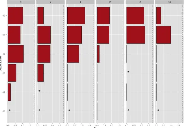
Figure 6 – Maximum hydrolysis rate (nmol L-1 h-1) measured for the six high-molecular-weight polysaccharide substrates at each station (horizontal panels) and depth (vertical panels). Bar height indicates mean hydrolysis rate; black circles indicate rates measured for each individual triplicate incubation. Error bars are standard deviation of the three triplicate measurements. Where black circles are absent, hydrolysis rates were 0 in all three triplicate
incubations at all timepoints. Asterisk at Station15-d2-xyl indicates missing data.
Patterns in Polysaccharide-Hydrolyzing Enzyme Activities with Depth, Latitude, and Time
Broad patterns in polysaccharide hydrolysis are evident. Generally, hydrolysis rates decreased with depth (Figure 6, Figure 7), and the spectrum of substrates measurably
Figure 7 – Hydrolysis activity for individual (colored points) and summed (grey shading) substrates (nmol/L*hr) on the y axis versus Latitude (station) on the x axis, by depth (horizontal panels). Mean values are symbolized by the points with standard deviation of individual measurements by the error bars. Colors indicate individual substrates; the grey curve is the sum of the mean maximum hydrolysis rates of all six substrates at that depth and station.
Index H (which is a measure of “hydrolytic diversity” taking both the spectrum of substrates hydrolyzed as well as the evenness of their relative rates of hydrolysis into account) were much lower at depths below 250m (Figure 4, Figure 8). The decrease in the Shannon Diversity Index with depth is more pronounced at stations with strong stratification: Stations 15 and 18, where stratification is strongest (Appendix B), drop from relatively high Shannon indices at the DCM to 0 at mesopelagic depths, whereas at Stations 2 and 4 where stratification is weakest Shannon indices decrease more gradually with depth (Figure 8).
Figure 8 – Shannon indices (H) for all incubation sets, visualized by station and depth. Asterisks indicate N/A where
H could not be calculated (where no hydrolysis was detected). Maximum Shannon Index is 1.79, indicated by dashed line. Where a black line but no red is visible, H is 0 (only one substrate was hydrolyzed).
every station, and at every depth in the upper 250m of the water column; laminarin hydrolysis rates decreased considerably with depth, but hydrolysis was observed at five out of six stations in AAIW and NADW waters, and was the only substrate measurably hydrolyzed in Bottom water (at Station 10 only, 0.12 ± 0.15 nM/hr). Laminarin and chondroitin were the only substrates measurably hydrolyzed below 250m in AAIW, NADW, and Bottom waters. Chondroitin hydrolysis in these deep waters was observed only at Stations 2 and 4, while low levels of laminarin hydrolysis in deep waters was more ubiquitous. Pullulan and xylan hydrolysis was confined to the upper 250m; pullulan hydrolysis occurred in shallow water at all stations while xylan hydrolysis was more variable, being hydrolyzed at all stations except Station 2.
Summed hydrolysis rates – the sum of the maximum hydrolysis rate of all six substrates at a given station and depth – also showed considerable variation (Figure 7). Higher summed hydrolysis rates corresponded with higher hydrolytic diversity H (Appendix C). The
northernmost stations (Stations 10, 15, and 18) tended to have higher summed hydrolysis rates at Surface and DCM depths relative to the southernmost stations (Stations 2, 4, 7), while
mesopelagic hydrolysis rates were higher at the southernmost stations than the northernmost (Figure 7). The difference in summed hydrolysis rate between DCM and mesopelagic depths varied by station as well – at the southernmost stations, hydrolysis was similar at both the DCM and mesopelagic depths, while at the northernmost stations hydrolysis was higher at the DCM relative to mesopelagic depths.
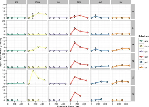
Figure 9 – Representative plot (in surface water only) of how enzymatic response to substrate addition varied on
different timescales. Surface water hydrolysis rates (y axis) measured at each timepoint (x axis) for each substrate (vertical panels) at each station (horizontal panels). Enzymatic response time of the microbial community to the added substrate (timepoint at which maximum hydrolysis activity occurs) varied considerably by substrate and by incubation. Maximum hydrolysis rates (e.g. Station2-chon-T2) are therefore used to compare among incubations.
Influence of Environmental Parameters on Hydrolytic Activities
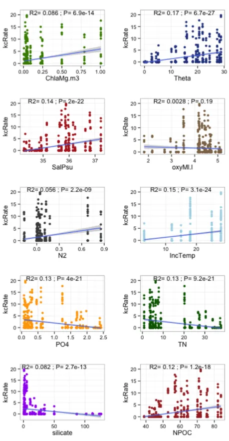
Figure 10 – Correlation between kill-corrected maximum hydrolysis rates for all individual replicates (not mean
Linear relationships between aggregate maximum hydrolysis rates (including all substrates together) and environmental parameters are generally weakly correlated (R2<0.2,
Figure 10). The strongest correlation is with in situ potential temperature (R2=0.17, P<0.001),
but correlations of similar strength exist between hydrolysis rate and salinity, phosphate, TN, DOC, and incubation temperature. Individual substrates are correlated with environmental variables at varying strengths (Appendix D). However, many of these environmental parameters co-correlate strongly with one another (e.g. potential temperature is correlated with DOC, R2=0.85).
Figure 11 – Best fit multiple linear regression model of hydrolysis activity explained by environmental variables.
An analysis of variance multiple linear model was used to assess the environmental parameters best correlated with hydrolysis rates, accounting for co-correlations among environmental parameters themselves. Best fit ANOVA multiple regression models for aggregate hydrolysis rates (including all six substrates together), and for each substrate individually revealed the environmental parameters most strongly correlated with hydrolytic activity (Figure 11, Figure 12, Appendix E). Typically, one or two environmental parameters correlated with hydrolysis rates almost as well as a linear model including all 10 parameters (Appendix E) so these one or two parameters were used for ANOVA models (Figure 11, Figure 12). Potential temperature correlated best with hydrolysis when all substrates were considered together (R2=0.17), and including both temperature and chlorophyll was the best-fit model
(R2=0.19, Figure 11). However, when substrates were considered individually, different
environmental parameters gave the best fit (Figure 12). Chondroitin was best correlated with temperature alone (R2=0.20), laminarin with temperature and chlorophyll (R2=0.78), pullulan
with temperature and buoyancy frequency (R2=0.45), and xylan with chlorophyll and salinity
(R2=0.41). Models were not made for arabinogalactan and fucoidan, for which little or no activity
Figure 12 – Best fit multiple regression models for hydrolysis rates specific to individual substrates chondroitin (top
left), laminarin (top right), pullulan (bottom left), and xylan (bottom right). Fucoidan and arabinogalactan are not shown because zero or very little activity was detected at all depths and stations. Chondroitin is best explained by potential temperature alone by the formula chonRate = -0.469 + 0.189(Theta); laminarin is best explained by potential temperature and chlorophyll by the formula lamRate = -0.327 + 0.415(Theta) + 4.367(Chla); pullulan is best explained by potential temperature and buoyancy frequency by the formula pulRate = -0.287 + 0.076(Theta) +
3.606(N2); and xylan is best explained by chlorophyll and salinity by the formula xylRate = -57.08 + 7.360(Chla) +
1.642(Sal). Correlation coefficients and P-values for each model are annotated within the plot – the strength of the
relationship varies, but all relationships are highly significant.
Connectivity of Hydrolytic Assemblages Among Depths vs. Stations
A Bray-Curtis dissimilarity matrix was made to compare the hydrolysis assemblages of each site from Surface, DCM, and Mesopelagic depths. This matrix was represented using Non-Parametric Multidimensional Scaling to visualize and compare dissimilarities among sites (Figure 13, Figure 14). BC dissimilarities among sites are significantly affected when grouped by station (Figure 13, P=0.008), but not when grouped by depth (Figure 14, P=0.42).
Figure 13 – Nonparametric Multidimensional Scaling visualization of Bray-Curtis distances among enzyme activity
assemblages in surface, DCM, and mesopelagic sampling depths at all stations. Ellipsoids are grouped by station and a point within the ellipsoid represents the surface, DCM, or mesopelagic depth at that station. Coordinates of the ellipse are determined by the standard deviation of the points. The mesopelagic depth at station 15 is not included because missing xylan hydrolysis data prevents the calculation of BC dissimilarities against other stations. Station has a significant effect on the variation in Bray-Curtis distances – e.g. assemblages of enzyme activity at a single station are more similar to each other than to all sites in general (P=0.008).
Figure 14 – Nonparametric Multidimensional Scaling visualization of Bray-Curtis distances among enzyme activity
Enzymatic Hydrolysis of Monomeric Substrates
Patterns in Leucine Aminopeptidase Activities with Depth, Latitude, and Time
MCA-leucine hydrolysis was ubiquitous over all depths and stations (Figure 15).
Hydrolysis rates of leucine ranged from zero to 18.0 nM/hr, although 93% of rates were below 5 nM/hr, and 66% of rates were below 1 nM/hr.
Figure 15 – Leucine aminopeptidase hydrolytic activity vs. latitude (station) for each depth (vertical panels).
Leucine aminopeptidase activity generally decreased with depth from surface to bottom water at all stations (Figure 16). At some stations (Stations 4, 7, 22, 23), maximum leucine aminopeptidase activity was in surface water, while at other stations (Stations 2, 10, 15, 18, 21) maximum activity was at the DCM. While activity was very low in deeper waters relative to shallower waters, hydrolytic activity was detected at all depths. Only two stations (Stations 2 and 21) showed zero activity in NADW water, while only two stations (Stations 2 and 7) showed zero activity in bottom water (depths of 5110 and 4513m, respectively). Activity ranged from 0 to 0.26 nM/hr in bottom water incubations across all stations, from 0 to 0.33 nM/hr in NADW, from 0.13 to 0.35 nM/hr in AAIW, and 0.29 to 1.16 nM/hr in mesopelagic water. Activity at the DCM ranged from 1.39 to 10.14 nM/hr, while surface water incubations ranged from 1.78 to 5.85 nM/hr.
Figure 16 – Maximum hydrolysis rate (nmol/L*hr) of leucine aminopeptidase with depth (y axis) at each station
(horizontal panels). Points represent mean rates; error bars are standard deviation of rates measured from triplicate incubations.
Aminopeptidase activities followed distinct trends across stations as well (Figure 15). Generally, aminopeptidase activity was highest in surface water and DCM incubations at stations surrounding the equator, with lower activity in the subtropical South Atlantic region. Additional peaks in activity were measured at 38°S (Station 2) and at 10°N (Station 23).
MCA-leucine hydrolysis rate also varied throughout the timecourse of an incubation. MCA-leucine hydrolysis is measured as an increase in fluorescence over time (see Methods), but that increase is not linear between each timepoint, resulting in variable hydrolysis rates over time. Leucine-MCA hydrolysis rates were typically at a maximum at the first timepoint and decreased over time (Figure 17). There were six incubations for which a maximum hydrolysis rate was at a timepoint later than T1 (Table 2). In these cases, the maximum hydrolysis rate was at the final timepoint.
Figure 17 – Representative trend of leucine aminopeptidase hydrolytic activity measured over the incubation
time course. Figure shown is from incubations with seawater from Station 2, d1 (deep chlorophyll maximum).
Stn
Depth
Aminopeptidase Activity
at T1 (nmol/L*hr)
Maximum aminopeptidase
activity (T3) (nmol/L*hr)
2
Bottom
0.0 ± 0.00
0.10 ± 0.025
4
Mesopelagic 0.48 ± 0.019
0.76 ± 0.204
15
Surface
4.75 ± 0.210
18.03 ± 12.378
21
DCM
2.73 ± 0.105
7.02 ± 2.331
21
Mesopelagic 0.41 ± 0.120
0.69 ± 0.048
23
Surface
5.85 ± 0.349
8.19 ± 1.476
Table 2 – Leucine aminopeptidase activity at T1 compared to maximal rates at T3 for the six incubations for
0
2
4
6
8
10
12
14
0
10
20
30
Patterns in α-glucosidase Activities with Depth, Latitude, and Time
α-glucosidase activity was highly variable, with no hydrolysis detected in 60% of
incubations (Figure 18). MUF-α-glucose hydrolysis rates had a broad distribution and ranged from zero to 43.0 nM/hr, although 92% of rates were under 5 nM/hr, while 70% of rates were under 1 nM/hr. The frequency of zero hydrolysis rates is mainly due to the fact that α-glucose hydrolysis was never detected in seawater sampled below the mesopelagic (250m) sampling site (Figure 19).
Figure 18 – α-glucosidase hydrolytic activity vs. latitude (station) for each depth (vertical panels). Note y-axis scale –
α-glucosidase activities decreased with depth at all stations (Figure 19). Hydrolysis of MUF-α-glucose was not detectable in incubations below the mesopelagic at any station, even after 72 hours of incubation, suggesting that the microbial communities in these waters do not have the capacity to access this substrate within the timescales of these incubations.
Mesopelagic incubations were mixed in their response, with seven of the nine stations sampled showing no α-glucosidase activity by the final timepoint. The highest activity detected, however, was also from mesopelagic water at station 7, at 43 nM/hr. Hydrolysis rates in surface water incubations ranged from 1.84 to 12.23 nM/hr, DCM incubations from 1.93 to 6.64 nM/hr, and mesopelagic incubations from 0 to 43 nM/hr, with all deeper water incubations showing zero activity.
Figure 19 – Maximum hydrolysis rate (nM/hr) of α-glucosidase with depth (y axis) at each station (horizontal panels).
Latitudinal differences in maximum α-glucosidase activity are also evident (Figure 18). Surface and mesopelagic activity closely mirrored each other, with a notable maximum in activity at 22.5°S (Station 7). Patterns of activity in incubations from the DCM were distinct from surface and mesopelagic waters, with maximum activities at the DCM measured at 22.5°S (Station 2), 3.5°N (Station 18), and 8.25°N (Station 22).
MUF-α-glucose hydrolysis rates also followed a distinct pattern over the timecourse of an incubation (Figure 20). Hydrolysis (measured as an increase in fluorescence over time) was typically very low or zero at the first timepoint, but increased over time, with a maximum hydrolysis rate at the final timepoint. This trend was observed in all incubations with MUF-α-glucose.
Figure 20 – Representative trend of α-glucosidase hydrolytic activity measured over the incubation time course.
Figure shown is from incubations with seawater from Station 2, d1 (deep chlorophyll maximum).
0
1
2
3
4
5
6
7
8
9
10
0
20
40
60
80
DISCUSSION
Patterns in heterotrophic enzyme activity have been shown to vary as a function of latitude (Arnosti et al. 2011), and while far fewer studies have investigated variations in hydrolytic activity with depth, those few studies have identified trends with depth as well (Baltar et al. 2010, Steen et al. 2012, D’Ambrosio et al. 2014). The spatial variability of extracellular enzymatic activity in both surface waters and the deep ocean is increasingly recognized, but defining the processes driving these variations is challenging. There are many possible factors that may drive variability in extracellular enzymatic activity in the
environment, but there are, broadly speaking, two possible explanations that dominate the literature – environmental conditions, and microbial community capacities.
Early studies found that environmental parameters such as utilizable DOM (UDOM) availability were related to extracellular enzyme activity in heterotrophs (Chróst 1991), while several mesocosm studies observed mixed effects of nutrient and UDOM amendments on extracellular enzymatic activity (Nausch & Nausch 2000, Donachie et al. 2001, Allison & Vitousek 2005). The advent of improved molecular techniques has increased interest in the effect of community composition on extracellular enzymatic activity. Davey et al. (2001) found that both microbial community composition and extracellular enzymatic activity were stratified with depth in the upper 100m of the North Atlantic, while other studies found broad variability in enzymatic capabilities and hydrolysis rates in individual marine isolates (Martinez et al. 1996, Bong et al. 2009). Enzyme activity measurements coupled with comparative genomics and proteomics of cultures from the North Sea demonstrated that individual taxa may occupy distinct carbon-degrading niches within a single community (Xing et al. 2014).
DOM, and also found evidence of resource partitioning and succession within these taxa, emphasizing the importance of community dynamics in processing natural organic matter (McCarren et al. 2010, Teeling et al. 2012).
Biogeographical distributions of distinct marine microbial communities across latitudinal gradients are being described as sequencing efforts increase (Martiny et al. 2006, Fuhrman et al. 2008, Zinger et al. 2011). Fewer studies have looked at gradients in community composition with depth, but biogeographical distributions of microbial communities along depth gradients, as well as gradients in function and carbon metabolism, are also emerging (Delong et al. 2006, Shi et al. 2011). Meanwhile, stratification of enzymatic activities has been identified across latitude (Arnosti et al. 2011) as well as depth ranges (Baltar et al. 2010; Steen et al. 2012; D’Ambrosio et al. 2014). The increasing evidence for both functional stratification and stratification in microbial community composition along environmental gradients implies a potential relationship between the microbial community capacities and hydrolysis activities, but much work remains to elucidate the interactions between these processes.
Microbial community composition and environmental conditions are often interrelated, however, complicating the distinction between potential factors driving heterotrophic enzyme activity. Environmental conditions have at least partial influence on organizing microbial communities, since environmental distance is more strongly related to microbial community function than geographic distance (Jiang et al. 2012). Accurate modeling of global microbial diversity biogeography can be constructed using environmental parameters (Ladau et al. 2013). Additionally, certain environmental parameters often ‘define’ the characteristics of an
environmental region (e.g. the unique T-S-O characteristics of distinct water masses), making environmental parameters and geospatial variation easily confounded. The relationship between activity and environmental parameters as well as community composition has not often been studied in conjunction with one another, but where it has (Kellogg & Deming 2014), this interdependence is evident. In the study by Kellogg & Deming (2014), extracellular
of these factors differing by site, by cell-specific vs. bulk enzymatic activities, and by particle-associated vs. free-living bacteria.
Other factors in addition to environmental parameters and microbial community composition may contribute to patterns of heterotrophic extracellular enzyme activity in the marine environment. Long residence times of active free enzymes in the environment, for example, could significantly contribute to total hydrolysis, even where cell-associated activity is low (Steen & Arnosti 2011). Specific naturally-occurring free extracellular enzymes in the Arctic were found to have a lifetime of several days (Steen & Arnosti 2011), while cell-free enzymes have been observed to contribute to a large proportion of total hydrolysis at some sites in the open ocean (Baltar et al. 2010). Activities of free enzymes might have a significant impact on global heterotrophic activity, but relatively few studies have measured free-enzyme hydrolytic activity, and the associated residence times of those enzymes, in the marine environment (Steen & Arnosti 2011). These factors should also be taken into consideration as we work toward a more comprehensive picture of heterotrophic enzyme dynamics and the factors that drive it.
This study identifies geospatial patterns in extracellular enzymatic hydrolysis of high-molecular-weight organic matter across both latitudinal and depth regimes. Few studies have looked at as broad a span of latitude, and even fewer have looked at depth variations of
activities beyond the upper 100-250m of the water column. Hydrolysis of high-molecular-weight organic substrates is measured in addition to low-molecular weight substrates. Most studies focus on low-molecular-weight, ‘utilizable’ DOM (e.g. Davey et al. 2001, Kellogg & Deming 2014, Baltar et al. 2010), but high-molecular-weight organic substrates are more representative of natural organic matter (Warren 1996). Considering both high- and low-molecular-weight
substrates in the same study allows us to compare our results to previous studies while gaining unique insight into heterotrophic enzyme dynamics in the environment.
glucosidase and leucine aminopeptidase activities generally decreased with depth at every station, with a peak in activity at either the surface or the DCM (Figure 19, Figure 16). The stations at which hydrolysis was highest in shallow waters were variable for both substrates, and whether peak activity was at the surface or the DCM was also variable by station (Figure 18, Figure 15).
α-glucosidase activity was undetectable below 250m even after 72 hours of incubation,
even though activities in shallow waters were quite high, an observation that suggests that α-glucosidase enzymatic capacities of microbial communities in deeper water differ markedly from shallow waters. α-glucosidase activities were highly variable, however, and extremely high activities were measured in the upper 250m of the water column at some sites (Figure 19, Figure 18). These observations contrast with the trends observed by Baltar et al. (2010), who observed modest α-glucosidase activities in the epipelagic that decreased with depth but remained relatively high in deep water. However, their study apparently did not include killed controls in the experimental setup, which are necessary to remove any effect of non-hydrolytic auto-fluorescence of the fluorogenic substrate (Hoppe 1983), and this may account for the high activity rates observed with depth in Baltar et al. (2010). In shallow water, we observed peak activities typically at the DCM or at the surface, but they did not correspond to the degree of stratification at that site (Figure 18). The highest α-glucosidase rate detected, however, was 41 ± 43 nM/hr at the Mesopelagic depth at Station 7. This is an extremely high rate with a very high standard deviation; the high standard deviation is due to one replicate incubation in which very high activity was measured, while very low activity was measured in the other two replicates, so it seems likely that an aggregate or other particulate in one replicate resulted in the high
activity observed.
Despite notable differences (high activities with depth), results from previous studies investigating activities of extracellular enzymes that hydrolyze low-molecular-weight substrates in the South Atlantic are generally consistent with the results obtained in this project,
particularly in shallower waters. However, the activities observed using low-molecular-weight substrates are not likely to reflect natural extracellular enzyme activities (Warren 1996) that depend on the particular conformations and substrate specificities of enzymes targeting complex, high-molecular-weight organic matter.
This study illuminates patterns of high-molecular-weight substrate hydrolysis that are characteristic of individual substrates: some substrates are hydrolyzed at almost all stations and depths, some are ubiquitous across stations but hydrolyzed only in shallow waters, some are patchy and are hydrolyzed at some stations but not others, while some are rarely degraded at any site (Figure 6). The spectrum of substrates hydrolyzed at each site and the evenness of their rates of hydrolysis (as indicated by the Shannon Diversity Index) decreases with depth (Figure 8). The sites with highest hydrolytic diversity were also the sites of highest summed hydrolysis rates (Figure 7), e.g. Station15-Surface and Station15-DCM (R2=0.71, P<0.001,
Appendix C). At the northernmost stations, summed hydrolysis as well as Shannon Diversity (H) decreased more quickly with depth than at the southernmost stations. This difference may be partially due to differences in stratification – the northernmost stations were more stratified at the pycnocline (peak buoyancy frequencies were higher) than the southernmost stations (Appendix B). Indeed, there is a weak, marginally significant (R2=0.58, P=0.08) negative
correlation between maximum buoyancy frequency at the pycnocline and the difference between summed hydrolysis at mesopelagic and DCM water (Appendix F).
Some substrates were not detectably hydrolyzed at several sites throughout the 21-day incubations. Fucoidan hydrolysis was not detected at any site and arabinogalactan was
timescale is insufficient to measure hydrolysis, which may be very low or may require a growth response from potentially slow-growing and/or rare members of the microbial community. In deep-water incubations, the latter explanation seems more likely. Generation times of deep-sea microbes may be on the order of 3-4 weeks (Wirsen & Molyneaux 1999), so if hydrolysis
depends on a growth response by particular, potentially rare microbial groups, an extended time course may be necessary in future studies to obtain a more robust and accurate picture of deep-water open-ocean enzymatic capacities. In a study that measured hydrolysis of these same polysaccharides at depths extending to ca. 900 m (the deepest depth published to date), similar effects were observed (Steen et al. 2012).
Many of the hydrolysis rates measured in this study have high standard deviations. This is usually due to one experimental replicate that showed high activity, while the other two replicates did not hydrolyze the added substrate (Figure 6). This result suggests that the capacity to hydrolyze a particular organic substrate may be heterogeneously distributed. This observation is consistent with the hypothesis that members of the rare biosphere may
contribute disproportionately to the breakdown of complex organic carbon (Steen et al. 2012), a testable hypothesis that should be pursued in future studies. Another possibility is that a small aggregate or other particulate may have gotten into one replicate and not in the others,
producing high activity in one triplicate.
Differences in the timing of enzymatic responses to different substrates (Figure 9) imply differences in growth response or rates of gene expression by those members of the heterotrophic community able to access the substrate. A delay in response to the added substrate may be due to the need to enrich particular members of the rare biosphere before hydrolysis is detectable, or differences in cell signaling which regulates hydrolytic enzyme expression (Arnosti 2011, Steen et al. 2012). Whether this is an accurate explanation for the variability in enzymatic activity observed in this and other studies is an important question for future work.
The pattern among these assemblages is observable in Figure 6; it appears that assemblages are more similar at different depths within the same station than they are within the same water depth across all stations. This pattern is particularly evident in the upper 250m of the water column.
The Bray-Curtis (BC) dissimilarity is a useful index to test this observation statistically, which quantifies how dissimilar the “species” (in this case, substrate hydrolysis) compositions of two different sites are. BC dissimilarities cannot be calculated between sites where no hydrolysis was detected at either site, so only the surface, DCM, and mesopelagic depths were considered for this analysis where activities were robust.
The BC dissimilarity matrix for these sites is represented by Euclidean distances between points in Figure 13 and Figure 14. Points (sites) closer to each other are more dissimilar (have a higher BC index). When sampling sites are grouped by station (Figure 13), they appear to cluster more closely with each other, and more independently from other clusters, than when sites are grouped by depth (Figure 14). Indeed, this observation is borne out statistically – permutational ANOVA (PERMANOVA) finds that station has a significant effect on the variation in the BC dissimilarity matrix (P=0.008), while depth does not (P=0.42). This result suggests that enzyme activities have higher vertical connectivity than horizontal at these sites, which may suggest that vertical sinking is more important than advection in the epipelagic in transferring hydrolytic capabilities.
applied to the deep open ocean – extending the time course of deep-water incubations in future experiments may overcome this obstacle.
The statistical relationships observed between environmental parameters and heterotrophic enzyme activity in this study may seem straightforward at first glance, but at closer inspection suggests a more complex set of driving mechanisms. When all substrates are considered together, environmental parameters poorly explain hydrolysis activity (R2<0.2,
Figure 10). The correlations of individual substrates with environmental variables, particularly temperature, match very closely the correlation coefficients observed in previous studies (Arnosti et al. 2011). The data presented here corroborate previous observations and suggest that biogeographical distributions of enzymatic activities, and the extent to which environment influences them, are consistent across oceanographic regions.
The relationships between the ten environmental parameters considered in this study (Figure 10, Figure 11) and hydrolysis activity are highly statistically significant (in most cases, P<10-5, and in all cases P<10-3), although the scientific interpretation of that statistic is less straightforward. A particular independent variable correlated to hydrolytic activity with an R2=0.5 does not mean that variable directly led to 50% of the activity observed. For example, it
does not seem logical that xylan hydrolysis is directly driven by low chlorophyll and high salinity, as the multiple linear regression suggests (Figure 12). Xylan is found in both terrestrial and marine environments, as the second most abundant component of plant cell walls
with water depth. Pullulan, similarly, is hydrolyzed at every station, but exclusively above either 250m or DCM depths. The stations where pullulan is not hydrolyzed below the DCM
correspond with the most highly stratified stations near the equator where buoyancy frequency is higher in shallower waters, and stations with pullulan hydrolysis at 250m corresponds to less stratified stations (Figure 6, Figure 4b, Appendix B). Thus, the fact that its strongest
relationship with environmental parameters is between temperature and buoyancy frequency (Figure 12, Appendix E) is logical, even though it is unlikely that buoyancy frequency itself causes pullulanase activity.
The best-fit correlation of individual substrates with differing environmental variables, then, may instead be a reflection of the co-occurring geospatial variability in both hydrolytic activity and in environmental parameters. We can see that individual substrates are hydrolyzed in distinct geospatial patterns (Figure 6), and physicochemical parameters also vary spatially (Figure 3, Figure 5), so a combination of environmental parameters may do an intermediate job of describing the spatial variability of activity data, even if those parameters have no direct effect on enzyme expression.If physicochemical parameters exerted direct control on the biochemistry of extracellular enzyme activity, a more consistent set of variables would be able to predict all enzyme activity, rather than the varying combinations of variables observed. This suggests that an alternative explanation – such as microbial community composition or
functional capabilities – exerts a more direct control over extracellular enzyme activity. Environmental conditions may still be indirectly related to extracellular enzymatic activity, insomuch as environment contributes to shaping microbial communities (Jiang et al. 2012), but the statistical relationship between environmental variables and enzyme activity should be interpreted with caution.
This does not rule out the possibility, however, that environmental variables may be important for the hydrolysis of particular substrates – in particular those for which
between laminarin and temperature has been observed in other studies as well (Arnosti et al. 2011). This strong correlation may in fact be due to its ubiquitous hydrolysis, which suggests that the capacity to hydrolyze laminarin is globally distributed, thereby potentially dampening the influence of contributing factors such as community composition and leading to an
increased importance of other potential drivers (environment). Other substrates, which are less strongly correlated to environmental variables, are hydrolyzed less ubiquitously, perhaps due to differences in microbial community capacity to access the substrate, and thus may be more strongly driven by microbial community factors and not environmental factors.
We must ask, in this case, why laminarinase activity in particular is so widely
distributed. Laminarin and pullulan are both polysaccharides made of glucose subunits, but only laminarin is hydrolyzed ubiquitously, so it is not likely to be due to differences in monomeric composition. Perhaps ubiquitous laminarinase activities are due instead to the ubiquitous production of laminarin – laminarin is the primary storage glucan in diatoms, and is produced in high abundances estimated to be between 5-15 billion metric tons annually
(Alderkamp et al. 2007). The abundance of laminarin in the environment may thus explain the favorability of maintaining the capacity to hydrolyze laminarin in natural heterotrophic communities. If this is true, it follows that other cosmopolitan substrates will be hydrolyzed ubiquitously, while less abundant substrates will have “patchier” hydrolysis distributions. This is a difficult question to answer due to the current methodological limitations in determining organic carbon composition (Nebbioso & Piccolo 2012), but an important line of inquiry for future study nonetheless.