arXiv:1511.09361v2 [cond-mat.quant-gas] 17 Jun 2016
essential properties from few- to many-body
Lukas Rammelm¨uller,1, 2,∗ William J. Porter,2,† and Joaqu´ın E. Drut2,‡
1
Institute of Solid State Physics, Vienna University of Technology, A-1040 Vienna, Austria 2
Department of Physics and Astronomy, University of North Carolina, Chapel Hill, NC, 27599, USA (Dated: April 11, 2018)
We calculate the ground-state properties of unpolarized two-dimensional attractive fermions in the range from few to many particles. Using first-principles lattice Monte Carlo methods, we deter-mine the ground-state energy, Tan’s contact, momentum distribution, and single-particle correlation function. We investigate those properties for systems of N = 4,8, ...,40 particles and for a wide range of attractive couplings. As the attractive coupling is increased, the thermodynamic limit is reached at progressively lowerN due to the dominance of the two-body sector. At large momentak, the momentum distribution displays the expectedk−4
behavior, but its onset shifts fromk≃1.8kF at weak coupling towards higherkat strong coupling.
PACS numbers: 03.65.Ud, 05.30.Fk, 03.67.Mn
I. INTRODUCTION
Precise experiments with ultracold atomic fermion clouds are currently being carried out by several groups around the world. Among the systems in the ever-expanding set that such experiments can study, it is now possible to probe two-dimensional (2D) physics in a clean and controllable way [1–3]. This is an exciting opportu-nity to understand key aspects of few- and many-body quantum physics that are not specific to atoms but which are generic to 2D quantum mechanics.
Such phenomena include the classical scale invariance displayed by non-relativistic fermions in 2D, which is broken by quantum fluctuations (i.e. the symmetry is anomalous, see [4]), a property shared with four-dimensional gauge theories like quantum chromodynam-ics [5]. Although finite-temperature symmetry-breaking transitions are not possible for continuous symmetries in 2D (as explained by the Mermin-Wagner theorem [6]), at-tractive interactions do result in a Berezinskii-Kosterlitz-Thouless (BKT) transition into a low-temperature su-perfluid phase [7], which is another feature generic to 2D systems. High-temperature superconductivity is also understood to be essentially a 2D phenomenon [8], and it shares with ultracold atoms the so-called pseudogap regime [9]. Last, but not least, the recent excitement about the physics of graphene is also associated with scale invariant 2D systems, and with its affinity with relativis-tic strongly coupled matter [10].
Thus, the realization and exploration of flat ultra-cold atomic clouds impacts a wide range of areas in physics, and in the last few years this research has been pursued vigorously (see Refs. [11, 12] for recent wide-audience reports). On the experimental side, two-dimensional fermionic clouds were first achieved just a
few years ago in [13, 14], and many properties, rang-ing from spectroscopy to thermodynamics and hydrody-namic response, have been studied since [15–28].
On the theory side, early work in 2D used mean-field approaches to study the crossover between Bose-Einstein condensation (BEC) and BardeCooper-Schrieffer (BCS) pairing [29–31]. The ground-state en-ergy and contact were computed in the thermodynamic limit in Ref. [32] using the diffusion Monte Carlo method, which was updated and expanded by Refs. [33, 34] with a precise ab initio study of multiple ground-state prop-erties. Studies at finite temperature have also appeared (see e.g. [35–44]).
Thus, a fair amount is known about the many-body physics of these systems; however, much less is known about their few-body properties and how they approach the thermodynamic regime. In this work, we calcu-late from first principles some of the most important ground-state properties characterizing this few-to-many crossover: the energy, Tan’s contact, the momentum dis-tribution, and the single-particle propagator.
II. HAMILTONIAN AND COMPUTATIONAL APPROACH
Since our intent is to focus on non-relativistic Fermi systems with short-range interactions, our Hamiltonian is given by
ˆ
H = ˆT+gVˆ (1)
where the kinetic and potential terms ˆT and ˆV are given by
ˆ
T = X
s=↑,↓ Z
d2xψˆ†
s(x)
−~
2∇2
2m
ˆ
ψs(x) (2)
and
ˆ
V =−
Z d2xnˆ
respectively, and where the spin-sfermionic field opera-tors are denoted with ˆψs and ˆψ†s, with associated
den-sities ˆns. From this point on, we use units such that ~=m=kB= 1, such thatgis dimensionless and ˆV has
dimensions of energy as written. Although no new di-mensionful parameters enter the dynamics of the system when the interaction is turned on, the classical scale in-variance is broken by quantum fluctuations, which result in a non-zero pair binding energy.
Given a stable many-body system, ground-state expec-tation values may be obtained from the large-imaginary-time properties of an arbitrary trial state|φ0i, so long as the latter is not orthogonal to the system’s true ground state. In this work, we take |φ0i to be a single Slater determinant made out of the lowest-energy plane-wave orbitals. While this choice can certainly be optimized, we find it to be sufficient for our purposes.
For an operator ˆO, we define
Oβ≡
hφ0|Uˆ(β, β/2) ˆOUˆ(β/2,0)|φ0i
hφ0|Uˆ(β,0)|φ0i
, (4)
where
ˆ
U(τb, τa)≡exp h
−(τb−τa) ˆH i
(5)
is the imaginary-time evolution operator. It follows im-mediately that Oβ
β→∞
−−−−→ hOˆi, where the expectation value on the right is in the true ground state of the sys-tem. For some observables, in particular the Hamilto-nian itself, this convergence can be easily shown to be monotonic inβ (in fact, exponential), which makes their acquisition to some extent straightforward.
To address the interaction, we approximate the imaginary-time evolution operators ˆU via a symmetric Suzuki-Trotter decomposition as
ˆ
U(τa+τ, τa) =e−τ
ˆ
T /2e−τ gVˆ
e−τT /ˆ 2
+O(τ3), (6)
again splitting the Hamiltonian into its relatively sim-ple one-body kinetic term and comparatively complicated two-body, zero-range potential term. While continuous-time approaches have been known for a long continuous-time [45], they have not yet been adapted to the hybrid Monte Carlo technique, which we prefer in order to make con-tact with lattice-QCD methods [46]. At each timestep, we decompose the central (potential energy, two-body) operator via a Hubbard-Stratonovich transformation [47] into a linear combination of products of one-body oper-ators writing (generically)
e−τ gVˆ = Z
Dσ e−τVˆ↑,σe−τVˆ↓,σ, (7)
for an auxiliary fieldσ(x) summed over all possible
con-figurations at each imaginary-time slice. The specific form of the operatorse−τVˆ
s,σ, fors=↑,↓, depends on the choice of Hubbard-Stratonovich transformation. In our
case, we have decoupled the interaction in the density-density channel using a continuous and compact auxiliary field (see e.g. Ref. [48] for further details).
In the above, we have implicitly assumed that the number of spatial degrees of freedom at each time step is finite. We accomplish this by taking space to be a square lattice, which results in a lattice field theory ap-proach in the same usual fashion as in lattice-QCD and Hubbard-model Monte Carlo calculations. The field inte-gral of Eq. (7) is estimated in practice using Metropolis-algorithm-based Monte Carlo methods, which is possi-ble as for unpolarized systems there is no sign propossi-blem. Further details can be found in Ref. [48]; closely related methods were used to examine systems in 1D in Ref. [49] and in 3D in Ref. [50].
In this work, we have used spatial lattice sizes of side
Nx= 24,28,32,36,40 points, and taken the spatial
lat-tice spacing to beℓ= 1 and the temporal lattice spacing
τ such thatτ /ℓ2= 0.01
−0.05. While the method is not limited by these parameters, we found them sufficient to achieve the continuum limit and to characterize the crossover from few- to many-body physics. On the other hand, the Monte Carlo estimation of the field integrals carries a statistical uncertainty. To reduce the latter, we took at least 500 decorrelated samples of the auxiliary field, such that the uncertainty can be expected to be of order 5% or less.
III. RESULTS AND DISCUSSION
To calibrate our lattice field theory, we solved the two-body problem for all values ofNxmentioned above and
determined the lattice binding energyεB as a function of the dimensionless couplinggand the lattice sizeNx.
Us-ing those results, we performed calculations for higher particle numbers N = 4,8,12, . . . ,40 at fixed physics as set by the renormalized couplingη = 1/2 ln(2εF/εB), whereεF=k
2
F/2 is the Fermi energy,kF=
√
2πnis the Fermi momentum, andn=N/L2is the total density. To ensure that our results are converged to the ground state, we followed the procedure outlined above of calculating at finiteβ and extrapolating toβ→ ∞.
In Fig.1, we show our results for the energy (extrap-olated to infinite volume), in units of the energy of the noninteracting caseEFG=
1
−0.5 0.0 0.5 1.0 1.5 2.0 2.5 3.0
0 10 20 30 40 50
[E/E
FG
] / [
εB
/
εF
] − 1
N
η = −1.5
η = −1.0
η = −0.5
η = 0.0
η = 0.5 −0.5
0.0 0.5 1.0 1.5
E/E
FG
η = 0.5
η = 1.0
η = 2.0
η = 3.0
η = ∞
FIG. 1. (color online) Ground-state energy E of N = 4,8,12, ...,40 unpolarized fermions, for several values of the dimensionless coupling η = −1.5,−1.0, . . . ,3.0,∞, the final corresponding to a free system. Top panel shows E for the four weakest couplings we calculated, in units of the energy of the noninteracting system EFG =
1
2N εF. Bottom panel displays E for the strongest couplings we considered, using the binding energy per particleεB/2 as a scale. Clearly, for
η <0 the energy per particle is dominated by the pair binding energy across all particle numbers. In both plots, the ground-state energy results of Ref. [33] in the thermodynamic limit are shown with solid squares atN= 50.
subtracted the binding energy per particleεB/2 from the total energy per particle in the bottom panel. Indeed, for η ≤ 1.0, the onset of the BEC regime implies that the energy is expected to be dominated by the binding energy of the pairs, which form immediately upon turn-ing on the interaction. The numerical results plotted in Fig.1are given in Appendix B, TableII.
While the ground-state energy is an essential quan-tity in any few- and many-body problem, more detailed information about the short-distance behavior of the sys-tem can be obtained from Tan’s contactC[53]. Indeed, it has been shown that C controls the high-momentum tail of the momentum distribution (see below) [54], as well as multiple sum rules of real-time response func-tions [55]. The calculation of C itself, however, involves a many-body problem that requires computational ap-proaches [51,56]. The contact obeys an adiabatic theo-rem (see [57,58]), which indicates thatCis proportional
to the change in the ground-state energyE with the s-wave scattering lengtha0. In our Hamiltonian Eq. (1), the scattering length enters fully through the bare cou-pling g (and, of course, the UV lattice cutoff, which we hold constant). Therefore,
C∝∂ln(∂Ek
Fa0) = ∂E
∂g ∂g ∂ln(kFa0)
. (8)
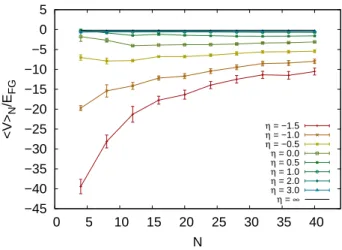
The factor ∂g/∂ln(kFa0) is a derivative at constant N that depends only on two-body physics, as the bare cou-pling g is determined by tuning to the desired a0 by solving the two-body problem. The ∂E/∂g factor, on the other hand, encodes many-body correlations and de-pends on the particle contentN. Because we have used a contact interaction [see Eq. (1)], the expectation value of the potential energy gives us access to∂E/∂gthrough the Hellmann-Feynman relation for theN-body problem:
hVˆiN = ∂E
∂g. (9)
In Fig. 2, we show hVˆiN in units of the ground-state
energy of the noninteracting gasEFG and as a function of both particle number and coupling. The numerical results plotted here are given in Appendix B, TableIII.
In Fig.3, we show our results for the momentum dis-tribution as a function ofk/kFforN = 36 particles and for several values of the dimensionless coupling η, ex-trapolated to β → ∞ (i.e. the ground state). Data at finite β are shown in Appendix A. The inset shows the same data in log-log form along with fits of the expected power lawk−4 (see e.g. Ref. [59]), which yield the con-tact at k ≫ kF. The expected behavior is obtained at weak coupling, but the region where it is valid becomes
−45 −40 −35 −30 −25 −20 −15 −10 −5 0 5
0 5 10 15 20 25 30 35 40
<V>
N
/E
FG
N
η = −1.5
η = −1.0
η = −0.5
η = 0.0
η = 0.5
η = 1.0
η = 2.0
η = 3.0
η = ∞
0.0 0.2 0.4 0.6 0.8 1.0
1.0 2.0 3.0 4.0 5.0 N = 36
n(k/k
F
)
k/kF
η = 3.0
η = 2.0
η = 1.0
η = 0.5
η = 0.0
η = −0.5
η = −1.0
η = −1.5
η = −2.0
η = ∞
10−5 10−3 10−1
2 4 8
FIG. 3. (color online) Momentum distribution of N = 36 unpolarized fermions, as a function ofk/kF, for several values of the dimensionless couplingη =−2.0,−1.5, ...,3.0, as well as the noninteracting case. Inset: Momentum distribution in log-log scale, showing the power-law decay that heals to a
∼(k/kF)−4
decrease at large k.
increasingly limited (i.e. it moves toward highk/kF) at strong coupling. Thus, in order to see the expected mo-mentum tail at strong coupling, calculations at larger vol-umes (lower kF) are needed. For most of the couplings we studied, however, it appears that the k−4 decay is reached around k/kF ≃ 1.8−2.0, which is remarkably close to its 3D counterpart [56].
In Fig.4, we show our results for the one-body density matrixρ1 defined in our unpolarized system as
ρ1(x,x′) =hψˆ†
↑(x) ˆψ↑(x′)i=hψˆ †
↓(x) ˆψ↓(x′)i, (10)
given the figure as a function of the dimensionless dis-tance kFr, where r= |x−x′|, as we take into account
−0.2 0 0.2 0.4 0.6 0.8 1
0 1 2 3 4 5 6 7
N = 36
ρ1
(kF
r)/
ρ1
(0)
kF r
η = −2.0
η = −1.5
η = −1.0
η = −0.5
η = 0.0
η = 0.5
η = 1.0
η = 2.0
η = 3.0
η = ∞
FIG. 4. (color online) One-body density matrixρ1forN= 36 unpolarized fermions, as a function ofkFr, for several values of the dimensionless couplingη=−2.0, ...,3.0, along with the
η→ ∞(i.e. noninteracting) case.
translation and rotation invariance. The results shown are for N = 36 particles and cover several values of the coupling η. The localized shape of ρ1 around x = 0 at strong couplings is a direct manifestation of the for-mation of bound pairs, which in turn makes lattice ap-proaches to the problem more challenging: the presence of the lattice-spacing scale competes with the pair size, which must be properly resolved in order to obtain accu-rate results.
To encode the intermediate and short-distance (kFr <
3.0) shape of our numerical results forρ1, we fit the fol-lowing dimensionless form to the data of Fig.4:
f(kFr, η) = 2e−a pBr
J1(kFr)
kFr
, (11)
whereais a fit parameter used to interpolate across cou-plings, andpB =
√
2kFe−η is the binding momentum of the two-body system (see Table I for fit results). The exponential factor in Eq. (11) is motivated by the deep bound state in the BEC regime, where single-particle cor-relation lengths are expected to be governed by the in-verse binding momentum. The Bessel function factor, along with the denominator, corresponds to the nonin-teracting case in the continuum limit.(see Table I for fit results)
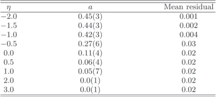
TABLE I. Fit parameter a obtained by fitting Eq. (11) to the data of Fig. 4, as a function of the dimensionless cou-plingη. The rightmost column shows the sum of the absolute value of the residuals per degree of freedom. These values of
aexemplify the typical numbers obtained across all particle numbers, i.e. beyond the data of Fig.4.
η a Mean residual
−2.0 0.45(3) 0.001
−1.5 0.44(3) 0.002
−1.0 0.42(3) 0.004
−0.5 0.27(6) 0.03
0.0 0.11(4) 0.02
0.5 0.06(4) 0.02
1.0 0.05(7) 0.02
2.0 0.0(1) 0.02
3.0 0.0(1) 0.02
IV. SUMMARY AND CONCLUSIONS
and the single-particle correlator. The ground-state en-ergy for each coupling strength forms a smooth curve with mild oscillations toward the thermodynamic limit. For η ≤ 0, particularly for N > 16, the ground-state energy is completely dominated by the binding energy of the pairs. Thus, the thermodynamic limit is reached much faster on the BEC side than on the BCS side. The momentum distribution approaches a (k/kF)−4decay at largek, as expected, but the onset of that behavior shifts noticeably towards large k as the coupling is increased. Finally, our fits to the single-particle correlation function
ρ1 indicate a shift from a kF-dominated region at weak
coupling, to apB-dominated region at strong coupling.
ACKNOWLEDGMENTS
We gratefully acknowledge discussions with E. R. An-derson and J. Kaufmann. This material is based upon work supported by the National Science Foundation un-der Grants No. PHY1306520 (Nuclear Theory pro-gram) and No. PHY1452635 (Computational Physics program).
V. APPENDIX A: FINITE-VOLUME EFFECTS AND EXTRAPOLATIONS
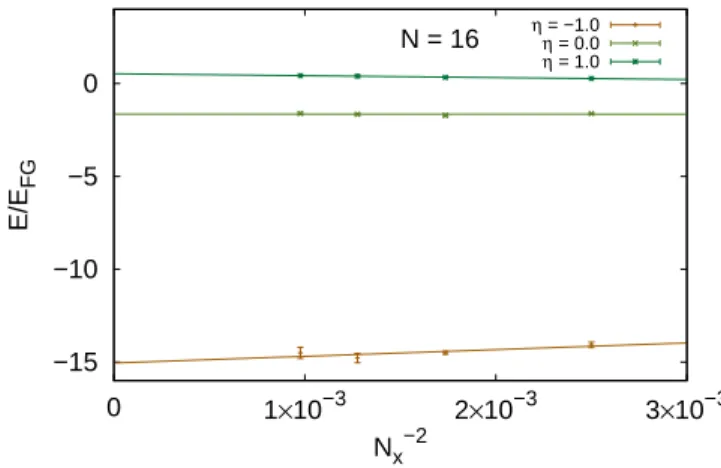
In this appendix we elaborate on the procedure we em-ployed to carry out extrapolations to the infinite volume limit, and present specific examples. In Fig. 5 we show the extrapolation forN = 16 particles for three different values of the dimensionless coupling η. To complement that example, we show in Fig. 6 the infinite-volume ex-trapolation for two different particle numbers at a fixed coupling.
−15 −10 −5 0
0 1×10⁻³ 2×10⁻³ 3×10⁻³ N = 16
E/E
FG
Nx−2
η = −1.0
η = 0.0
η = 1.0
FIG. 5. (color online) Extrapolation to the infinite vol-ume limit for N = 16 unpolarized fermions, as a func-tion ofN−2
x , for several values of the dimensionless coupling
η=−1.0,0.0,1.0.
0.05 0.1 0.15 0.2 0.25 0.3 0.35 0.4 0.45 0.5 0.55
0 1×10⁻³ 2×10⁻³ 3×10⁻³ η = 1.0
E/E
FG
Nx−2
N = 16 N = 32
FIG. 6. (color online) Extrapolation to the infinite volume limit forN= 16,32 unpolarized fermions at fixed dimension-less couplingη= 1.0, as a function ofN−2
x .
In Fig. 7 we show, for a specific coupling η = −0.5, the results of extrapolating our data for the momentum distributionn(k) to the ground state, which we accom-plish by increasing the length β of the imaginary time direction (i.e. the projection time). Clearly, such a cou-pling, though intermediate in strength, requiresβ ≃8.0 to start converging to the largeβ limit, in particular for the regionk < kF. One way to overcome such large
pro-jection times is to use a different guess for the ground-state wavefunction, as done for instance in Refs. [33,34].
0 0.2 0.4 0.6 0.8 1
0 1 2 3 4 5
N = 36 η = −0.5
n(k/k
F
)
k/kF
β = 0.5
β = 1.0
β = 1.5
β = 2.0
β = 3.0
β = 4.0
β = 5.0
β = 6.0
β = 7.0
β = 8.0
β = 9.0
β = 10.0
β = 12.0
β = ∞
FIG. 7. (color online). Momentum distribution extrapolated to infinite imaginary timeβforN = 36 unpolarized fermions on a 32×32 lattice and at fixed dimensionless couplingη=
VI. APPENDIX B: GROUND-STATE DATA TABLES
In this appendix we present tables showing our esti-mates for the ground-state energy and Tan’s contact as
a function of the couplingη=−1.5,−1.0, ...,3.0, for par-ticle numbers N = 4,8,12, . . . ,40, extrapolated to the infinite-volume limit.
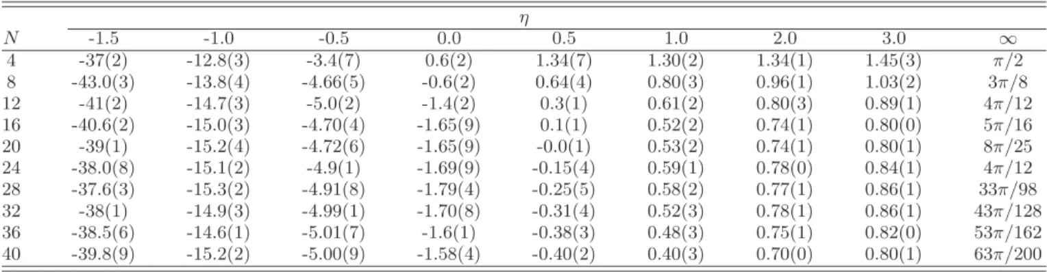
TABLE II. Ground-state energy E on the lattice, in units of the continuum noninteracting energy EFG = N εF/2 of the
N-particle system, as a function ofN and the dimensionless couplingη.
η
N -1.5 -1.0 -0.5 0.0 0.5 1.0 2.0 3.0 ∞
4 -37(2) -12.8(3) -3.4(7) 0.6(2) 1.34(7) 1.30(2) 1.34(1) 1.45(3) π/2
8 -43.0(3) -13.8(4) -4.66(5) -0.6(2) 0.64(4) 0.80(3) 0.96(1) 1.03(2) 3π/8
12 -41(2) -14.7(3) -5.0(2) -1.4(2) 0.3(1) 0.61(2) 0.80(3) 0.89(1) 4π/12
16 -40.6(2) -15.0(3) -4.70(4) -1.65(9) 0.1(1) 0.52(2) 0.74(1) 0.80(0) 5π/16
20 -39(1) -15.2(4) -4.72(6) -1.65(9) -0.0(1) 0.53(2) 0.74(1) 0.80(1) 8π/25
24 -38.0(8) -15.1(2) -4.9(1) -1.69(9) -0.15(4) 0.59(1) 0.78(0) 0.84(1) 4π/12
28 -37.6(3) -15.3(2) -4.91(8) -1.79(4) -0.25(5) 0.58(2) 0.77(1) 0.86(1) 33π/98
32 -38(1) -14.9(3) -4.99(1) -1.70(8) -0.31(4) 0.52(3) 0.78(1) 0.86(1) 43π/128
36 -38.5(6) -14.6(1) -5.01(7) -1.6(1) -0.38(3) 0.48(3) 0.75(1) 0.82(0) 53π/162
40 -39.8(9) -15.2(2) -5.00(9) -1.58(4) -0.40(2) 0.40(3) 0.70(0) 0.80(1) 63π/200
TABLE III. Ground-state interactionhVˆiN, in units of the energy of the non interacting gas EFG, as a function ofN and the dimensionless couplingη.
η
N -1.5 -1.0 -0.5 0.0 0.5 1.0 2.0 3.0 ∞
4 -39(2) -19.7(6) -7.0(7) -1(1) -0.1(2) -0.34(5) -0.50(1) -0.6(2) -1/(2π)
8 -28(2) -15(1.5) -7.9(7) -2.7(5) -0.86(9) -0.55(9) -0.41(1) -0.5(1) -1/(2π)
12 -21(2) -14.1(9) -7.8(3) -4.0(1) -1.47(4) -0.59(1) -0.42(4) -0.44(7) -1/(2π)
16 -17.7(1) -12.2(5) -6.8(1) -3.9(1) -1.2(2) -0.58(1) -0.38(2) -0.43(2) -1/(2π)
20 -16(1) -11.7(6) -6.8(3) -3.8(1) -1.44(8) -0.59(4) -0.41(2) -0.52(6) -1/(2π)
24 -14.0(9) -10.4(6) -6.4(3) -3.8(1) -1.55(1) -0.60(1) -0.41(1) -0.50(5) -1/(2π)
28 -12.5(9) -9.5(6) -6.0(4) -3.6(2) -1.67(3) -0.64(1) -0.44(1) -0.48(5) -1/(2π)
32 -11.4(9) -8.5(6) -5.6(3) -3.4(1) -1.68(1) -0.69(4) -0.41(1) -0.46(4) -1/(2π)
36 -11.5(1) -8.4(6) -5.6(3) -3.3(1) -1.65(1) -0.68(3) -0.40(2) -0.45(4) -1/(2π)
40 -10.5(9) -8.0(6) -5.4(3) -3.1(1) -1.59(2) -0.71(3) -0.41(2) -0.43(3) -1/(2π)
[1] Ultracold Fermi Gases, Proceedings of the Interna-tional School of Physics “Enrico Fermi”, Course CLXIV, Varenna, June 20 – 30, 2006, M. Inguscio, W. Ketterle, C. Salomon (Eds.) (IOS Press, Amsterdam, 2008). [2] I. Bloch, J. Dalibard, and W. Zwerger, Rev. Mod. Phys.
80, 885 (2008); S. Giorgini, L. P. Pitaevskii, and S. Stringari, Rev. Mod. Phys.80, 1215 (2008).
[3] J. Levinsen, M. M. Parish, Ann. Rev. Cold Atoms Mol. 3, 1 (2015).
[4] J. Hofmann, Phys. Rev. Lett. 108, 185303 (2012); E. Taylor and M. Randeria, Phys. Rev. Lett.109, 135301 (2012); Phys. Rev. Lett.110, 089904 (2013);
[5] J. R. Ellis, Nucl. Phys. B22, 478 (1970); R. J. Crewther, Phys. Lett. B33, 305 (1970); M. S. Chanowitz and J. R. Ellis, Phys. Lett. B40, 397 (1972); J. Schechter, Phys. Rev. D21, 3393 (1980); J. C. Collins, A. Duncan and S.
D. Joglekar, Phys. Rev. D16, 438 (1977); N. K. Nielsen, Nucl. Phys. B120, 212 (1977).
[6] N. D. Mermin and H. Wagner, Phys. Rev. Lett.17, 1133 (1966); P. C. Hohenberg, Phys. Rev. 158, 383 (1967); S. Coleman, Commun. Math. Phys.31, 259 (1973). [7] 40 Years of Berezinskii-Kosterlitz-Thouless Theory J.V.
Jose (Ed.) (World Scientific, Singapore, 2013); V. L. Berezinskii, Sov. Phys. JETP 34, 610 (1972); J. M. Kosterlitz and D.J. Thouless, J. Phys. C6, 1181 (1973); J. M. Kosterlitz, ibid.7, 1046 (1974).
[8] D. N. Basov and T. Timusk, Rev. Mod. Phys. 77, 721 (2005); S. A. Kivelson, I. P. Bindloss, E. Fradkin, V. Oganesyan, J. M. Tranquada, A. Kapitulnik, and C. Howald, Rev. Mod. Phys.75, 1201 (2003)
Q. Chen,et al.Phys. Rep.412, 1 (2005); K. Levin, and Q. Chen, in Ultracold Fermi Gases (Proc. Int’l School of Physics Enrico Fermi), Vol. CLXIV, 751 (2008); Y. He, et al.Phys. Rev. B 76, 224516 (2007), and earlier references therein; A. Peralli,et al.Phys. Rev. Lett. 92, 220404 (2004).
[10] V. N. Kotov, B. Uchoa, V. M. Pereira, F. Guinea, and A. H. Castro Neto, Rev. Mod. Phys.84, 1067 (2012). [11] M. Randeria, Physics5, 10 (2012).
[12] P. Pieri, Physics8, 53 (2015).
[13] K. Martiyanov, V. Makhalov, and A. Turlapov, Phys. Rev. Lett.105, 030404 (2010).
[14] M. Feld, B. Fr¨ohlich, E. Vogt, M. Koschorreck, and M. K¨ohl, Nature (London)480, 75 (2011).
[15] B. Fr¨ohlich, M. Feld, E. Vogt, M. Koschorreck, W. Zw-erger, and M. K¨ohl, Phys. Rev. Lett.106, 105301 (2011). [16] S.K. Baur, B. Fr¨ohlich, M. Feld, E. Vogt, D. Pertot, M. Koschorreck, and M. K¨ohl, Phys. Rev. A85, 061604 (2012).
[17] P. Dyke, E.D. Kuhnle, S. Whitlock, H. Hu, M. Mark, S. Hoinka, M. Lingham, P. Hannaford, and C. J. Vale, Phys. Rev. Lett.106, 105304 (2011).
[18] A. T. Sommer, L. W. Cheuk, M. J. H. Ku, W. S. Bakr, and M. W. Zwierlein, Phys. Rev. Lett. 108, 045302 (2012).
[19] Y. Zhang, W. Ong, I. Arakelyan, and J. E. Thomas, Phys. Rev. Lett. 108, 235302 (2012); M. Koschorreck, D. Pertot, E. Vogt, B. Fr¨ohlich, M. Feld, and M. K¨ohl, Nature (London)485, 619 (2012);
[20] A. A. Orel, P. Dyke, M. Delehaye, C. J. Vale, and H. Hu, New J. Phys.13, 113032 (2011).
[21] E. Vogt, M. Feld, B. Fr¨ohlich, D. Pertot, M. Koschorreck, M. K¨ohl, Phys. Rev. Lett.108, 070404 (2012).
[22] B. Fr¨ohlich, M. Feld, E. Vogt, M. Koschorreck, M. K¨ohl, C. Berthod, and T. Giamarchi, Phys. Rev. Lett. 109, 130403 (2012).
[23] P. Dyke, K. Fenech, T. Peppler, M. G. Lingham, S. Hoinka, W. Zhang, B. Mulkerin, H. Hu, X.-J. Liu, C. J. Vale, Phys. Rev. A93, 011603 (2016).
[24] V. Makhalov, K. Martiyanov, A. Turlapov, Phys. Rev. Lett.112, 045301 (2014).
[25] W. Ong, C. Cheng, I. Arakelyan, and J. E. Thomas, Phys. Rev. Lett.114, 110403 (2015).
[26] M. G. Ries, A. N. Wenz, G. Z¨urn, L. Bayha, I. Boettcher, D. Kedar, P. A. Murthy, M. Neidig, T. Lompe, and S. Jochim, Phys. Rev. Lett.114, 230401 (2015).
[27] P. A. Murthy, I. Boettcher, L. Bayha, M. Holzmann, D. Kedar, M. Neidig, M. G. Ries, A. N. Wenz, G. Z¨urn, S. Jochim, Phys. Rev. Lett.115, 010401 (2015).
[28] K. Fenech, P. Dyke, T. Peppler, M. G. Lingham, S. Hoinka, H. Hu, C. J. Vale, Phys. Rev. Lett.116, 045302 (2016); I. Boettcher, L. Bayha, D. Kedar, P. A. Murthy, M. Neidig, M. G. Ries, A. N. Wenz, G. Z¨urn, S. Jochim, T. Enss, Phys. Rev. Lett.116, 045303 (2016).
[29] K. Miyake, Prog. Theor. Phys.69, 1794 (1983).
[30] M. Randeria, J.-M. Duan, and L.-Y. Shieh, Phys. Rev. Lett. 62, 981 (1989); Phys. Rev. B 41, 327 (1990); S. Schmitt-Rink, C.M. Varma, and A.E. Ruckenstein, Phys. Rev. Lett.63, 445 (1989); M. Drechsler and W. Zwerger, Ann. Phys. (Leipzig)1, 15 (1992).
[31] W. Zhang, G.-D. Lin, and L.-M. Duan, Phys. Rev. A77, 063613 (2008).
[32] G. Bertaina and S. Giorgini, Phys. Rev. Lett. 106, 110403 (2011).
[33] H. Shi, S. Chiesa, and S. Zhang, Phys. Rev. A92, 033603 (2015).
[34] A. Galea, H. Dawkins, S. Gandolfi, A. Gezerlis, Phys. Rev. A93, 023602 (2016).
[35] X.-J. Liu, H. Hu, and P. D. Drummond, Phys. Rev. B 82, 054524 (2010).
[36] M. Bauer, M. M. Parish, and T. Enss, Phys. Rev. Lett. 112, 135302 (2014).
[37] V. Ngampruetikorn, J. Levinsen, and M. M. Parish, Phys. Rev. Lett.111, 265301 (2013).
[38] M. Barth and J. Hofmann, Phys. Rev. A 89, 013614 (2014).
[39] C. Chafin and T. Sch¨afer Phys. Rev. A88, 043636 (2013). [40] S. Chiacchiera, D. Davesne, T. Enss, and M. Urban,
Phys. Rev. A88, 053616 (2013).
[41] S. K. Baur, E. Vogt, M. K¨ohl, and G. M. Bruun, Phys. Rev. A 87, 043612 (2013).
[42] T. Enss, C. K¨uppersbusch, L. Fritz, Phys. Rev. A86, 013617 (2012).
[43] E. R. Anderson, J. E. Drut, Phys. Rev. Lett.115, 115301 (2015).
[44] B. C. Mulkerin, K. Fenech, P. Dyke, C. J. Vale, X.-J. Liu, H. Hu, Phys. Rev. A92, 063636 (2015).
[45] S. M. A. Rombouts, K. Heyde, and N. Jachowicz, Phys. Rev. Lett.82, 4155 (1999).
[46] S. Duane, A. D. Kennedy, B. J. Pendleton, D. Roweth, Phys. Lett. B 195, 216 (1987); S. A. Gottlieb, W. Liu, D. Toussaint, R. L. Renken, Phys. Rev. D 35, 2531 (1987).
[47] R. L. Stratonovich, Sov. Phys. Dokl. 2, 416 (1958); J. Hubbard, Phys. Rev. Lett.3, 77 (1959).
[48] D. Lee, Phys. Rev. C78, 024001 (2008); Prog. Part. Nucl. Phys.63, 117 (2009). J. E. Drut and A. N. Nicholson, J. Phys. G40, 043101 (2013).
[49] M. D. Hoffman, P. D. Javernick, A. C. Loheac, W. J. Porter, E. R. Anderson, J. E. Drut, Phys. Rev. A 91, 033618 (2015).
[50] A. Bulgac, J. E. Drut, and P. Magierski, Phys. Rev. Lett. 96, 090404 (2006); Phys. Rev. A78, 023625 (2008); J. E. Drut, T. A. L¨ahde, G. Wlazlowski, P. Magierski, Phys. Rev. A85, 051601(R) (2012).
[51] L. Rammelm¨uller, W. J. Porter, A. C. Loheac, J. E. Drut, Phys. Rev. A92, 013631 (2015).
[52] M. M. Forbes, S. Gandolfi, A. Gezerlis, Phys. Rev. Lett. 106, 235303 (2011).
[53] E. Braaten, in The BCS-BEC Crossover and the Uni-tary Fermi Gas, edited by W. Zwerger (Springer-Verlag, Heidelberg, 2012). X.-J. Liu Phys. Rep.524, 37 (2013). [54] S. Tan, Ann. Phys. 323, 2952 (2008); ibid. 323, 2971
(2008); ibid.323, 2987 (2008); S. Zhang, A. J. Leggett, Phys. Rev. A 77, 033614 (2008); E. Braaten, L. Plat-ter, Phys. Rev. Lett.100, 205301 (2008); E. Braaten, D. Kang, L. Platter,ibid.104, 223004 (2010);
[55] D. T. Son, E. G. Thompson, Phys. Rev. A81, 063634 (2010); E. Taylor, M. Randeria, Phys. Rev. A81, 053610 (2010).
[56] J.E. Drut, T.A. L¨ahde, T. Ten, Phys. Rev. Lett. 106, 205302 (2011); K. Van Houcke, F. Werner, E. Kozik, N. Prokof’ev, B. Svistunov, arXiv:1303.6245.
[57] F. Werner, Phys. Rev. A 78, 025601 (2008); C. Lang-mack, M. Barth, W. Zwerger, E. Braaten, Phys. Rev. Lett.108, 060402 (2012);