LOFAR sparse image reconstruction

DOI:10.1051/0004-6361/201424504 c

ESO 2015

Astrophysics

&

LOFAR sparse image reconstruction

H. Garsden

_{, J. N. Girard}

_{, J. L. Starck}

_{, S. Corbel}

_{, C. Tasse}

_{, A. Woiselle}

_{, J. P. McKean}

_,

A. S. van Amesfoort

_{, J. Anderson}

_{, I. M. Avruch}

_{, R. Beck}

_{, M. J. Bentum}

_{, P. Best}

_{, F. Breitling}

_,

J. Broderick

_{, M. Brüggen}

_{, H. R. Butcher}

_{, B. Ciardi}

_{, F. de Gasperin}

_{, E. de Geus}

_{, M. de Vos}

_{, S. Duscha}

_,

J. Eislö

ff

el

_{, D. Engels}

_{, H. Falcke}

_{, R. A. Fallows}

_{, R. Fender}

_{, C. Ferrari}

_{, W. Frieswijk}

_{, M. A. Garrett}

_,

J. Grießmeier

_{, A. W. Gunst}

_{, T. E. Hassall}

_{, G. Heald}

_{, M. Hoeft}

_{, J. Hörandel}

_{, A. van der Horst}

_,

E. Juette

_{, A. Karastergiou}

_{, V. I. Kondratiev}

_{, M. Kramer}

_{, M. Kuniyoshi}

_{, G. Kuper}

_{, G. Mann}

_,

S. Marko

ff

_{, R. McFadden}

_{, D. McKay-Bukowski}

_{, D. D. Mulcahy}

_{, H. Munk}

_{, M. J. Norden}

_{, E. Orru}

_,

H. Paas

_{, M. Pandey-Pommier}

_{, V. N. Pandey}

_{, G. Pietka}

_{, R. Pizzo}

_{, A. G. Polatidis}

_{, A. Renting}

_,

H. Röttgering

_{, A. Rowlinson}

_{, D. Schwarz}

_{, J. Sluman}

_{, O. Smirnov}

_{, B. W. Stappers}

_{, M. Steinmetz}

_,

A. Stewart

_{, J. Swinbank}

_{, M. Tagger}

_{, Y. Tang}

_{, C. Tasse}

_{, S. Thoudam}

_{, C. Toribio}

_{, R. Vermeulen}

_{, C. Vocks}

_,

R. J. van Weeren

_{, S. J. Wijnholds}

_{, M. W. Wise}

_{, O. Wucknitz}

_{, S. Yatawatta}

_{, P. Zarka}

_{, and A. Zensus}

(Affiliations can be found after the references) Received 30 June 2014/Accepted 18 December 2014

ABSTRACT

Context.The LOw Frequency ARray (LOFAR) radio telescope is a giant digital phased array interferometer with multiple antennas distributed in Europe. It provides discrete sets of Fourier components of the sky brightness. Recovering the original brightness distribution with aperture synthesis forms an inverse problem that can be solved by various deconvolution and minimization methods.

Aims.Recent papers have established a clear link between the discrete nature of radio interferometry measurement and the “compressed sensing” (CS) theory, which supports sparse reconstruction methods to form an image from the measured visibilities. Empowered by proximal theory, CS offers a sound framework for efficient global minimization and sparse data representation using fast algorithms. Combined with instrumental direction-dependent effects (DDE) in the scope of a real instrument, we developed and validated a new method based on this framework. Methods.We implemented a sparse reconstruction method in the standard LOFAR imaging tool and compared the photometric and resolution performance of this new imager with that of CLEAN-based methods (CLEAN and MS-CLEAN) with simulated and real LOFAR data.

Results.We show that i) sparse reconstruction performs as well as CLEAN in recovering the flux of point sources; ii) performs much better on extended objects (the root mean square error is reduced by a factor of up to 10); and iii) provides a solution with an effective angular resolution 2−3 times better than the CLEAN images.

Conclusions.Sparse recovery gives a correct photometry on high dynamic and wide-field images and improved realistic structures of extended sources (of simulated and real LOFAR datasets). This sparse reconstruction method is compatible with modern interferometric imagers that handle DDE corrections (A- and W-projections) required for current and future instruments such as LOFAR and SKA.

Key words.techniques: interferometric – methods: numerical – techniques: image processing

1. Introduction

Recent years have seen the development and planning of very large radio interferometers such as the LOw Frequency ARray (LOFAR; van Haarlem et al. 2013) in Europe, and the Square Kilometre Array (SKA;Dewdney et al. 2009) in Australia and South Africa (through its various precursors and pathfinders).

These new digital instruments have a very high sensitivity and a large field of view (FoV), as well as very large angular, temporal, and spectral resolutions in the radio spectrum observ-able from Earth. In particular, the very low frequency window (in the VHF – the very high frequency band between ∼10 and 250 MHz) is being explored (or revisited) with LOFAR, within the scope of various key science projects, spanning the search for fast transients (Stappers et al. 2011) to the study of early cos-mology (de Bruyn & LOFAR EoR Key Science Project Team 2012).

? _{Corresponding author: J. N. Girard,} e-mail:[email protected]

1.1. LOFAR

LOFAR is a digital radio interferometer composed of 48 stat-ions: 40 stations constitute the core and remote stations (two of which are future stations) that are distributed in the Netherlands (NL), and eight international stations that are lo-cated in Germany, Great Britain, France, and Sweden. Poland has planned the construction of three international stations that will enrich the array in the east-west direction. LOFAR has two working bands: the LBA-band (low-band antenna) from ≥30 to 80 MHz (that can be switched to 10−80 MHz), and the HBA-band (high-band antenna) from 110 to 250 MHz, lying on either-side of the FM band. One station consists of two arrays composed of fixed crossed dipole antennas, each offering a large FoV (therefore low directivity) and broadband properties1_{. The} HBA field of the core stations is split into two to increase the number of baselines.The stations measure induced electric sig-nals that undergo pre-processing operations in the station back-end, consisting of digitization, filtering, phasing, and summing.

1 _{See details atwww.lofar.org}

All these steps constitute the beamforming step of the phased antenna array. The output signal of one station is thus similar to that of a synthetic antenna whose beam is electronically pointed (rather than mechanically) in the direction of interest. Since most steps are performed in the digital side, multi-beam observations are possible and are only limited by the electronic hardware (i.e. in field-programmable gate arrays – FPGAs, by making trade-offs between the observed bandwidth and the number of numer-ical beams pointing at the sky).

At the interferometer level, the signal from every station is combined in a central correlator in the NL that performs a phased sum or inter-station cross-correlation. The latter operation en-ables LOFAR to build up a digital interferometer that samples a wide range of baselines (from∼70 m up to∼1300 km). The high flexibility of the instrument comes with the necessity of using advanced calibration strategies depending on the type of observations and its expected final sensitivity.

Since late 2012, LOFAR has been opened to the astronom-ical community by a regular public call for proposals2_{. Early} results with LOFAR demonstrated that it can reach a very high dynamic range (DR) on a wide FoV (i.e. several tens of degrees, see for exampleYatawatta et al. 2013) and a very high angular resolution (Wucknitz 2010;Shulevski 2010) at low frequencies. LOFAR capabilities are geared to key science projects on deep extragalactic surveys, transient radio phenomena and pul-sars, the epoch of reionization, high-energy cosmic rays, cosmic magnetism, and solar physics and space weather.

1.2. Increased complexity of low-frequency imaging

Since the beginning of radio interferometry imaging, various imaging methods have been designed to fit the requirements of different types of (extended) radio objects. The availability of high-performance computing and the need for efficient, fast, and accurate imaging for new wide-field interferometers has moti-vated the implementation of new imaging algorithms. Given the recording time and frequency resolutions, the integration time, and the diversity of baselines of wide-field interferometers, large amounts of data storage are required to save the telescope data. These data must then be transformed into a scientifically ex-ploitable form (typically into images cubes). Substantial compu-tational power is required for this as well (Begeman et al. 2011). Because of the nature and the dimensions of the LOFAR ar-ray, direction-dependent effects (DDE;Tasse et al. 2012) occur during the span of a LOFAR observation and add up to the usual other effects intervening in classical radio interferometers. These effects require a direction-dependent calibration before imaging. In particular, the classical compact planar array and small FoV assumptions are no longer valid, especially for a wide-field in-strument such as LOFAR. Modern calibration and imaging at radio wavelengths require a similar approach to that used in modern optical telescope with adaptive optics.

The problem can be generalized and expressed in the Measurement Equation framework (Sect. 2.5). The calibration problem therefore manifests as an inverse problem that should be solved to independently determine all the parameters and coefficients that describe each observation dataset.

Among the recent developments of data processing and re-construction algorithms, the discovery of compressed sensing (CS; Candès et al. 2006) has led to new approaches to solving these problems. It has been proposed for radio interferometry (e.g.Wiaux et al. 2009a;Wenger et al. 2010;Li et al. 2011a,b;

2 _{See the observation proposal section onwww.astron.nl}

Carrillo et al. 2012) because this constitutes a relevant practical case as a result of the sparse nature of the interferometric sam-pling (Sect.2.4).

The implementation of sparse radio image reconstruction methods is expected to produce better results on large extended objects with high angular resolution than other classical decon-volution methods. In Sect.2we first apply the theory of sparse reconstruction within the scope of radio aperture synthesis imag-ing and then implement it in the LOFAR imagimag-ing software. We also relate it to previous CLEAN-based deconvolution methods. We present in Sect.3the results of benchmark tests using sim-ulated and real LOFAR datasets by focusing on the quality of the image reconstruction compared to that of usual CLEAN-based algorithms. We then discuss the practical advantages and limitations of the current implementation and possible future developments.

2. Image reconstruction: from CLEAN to compressed sensing

2.1. Introduction

An ideal radio interferometer, composed of co-planar and iden-tical antennas, samples the sky in the Fourier domain (Wilson et al. 2009). In other words, each pair of antennas that forms one baseline gives access to the measure of the sky brightness as seen through a set of fringes with characteristics that depend on the frequency, the baseline length, and orientation with re-spect to the source. As for optical interferometers, the measured quantity (after correlating the pair of signals) is the fringe con-trast, also called (fringe) visibility. In the radio domain where the electric field varies slowly, we can sample both phase and amplitude with time and frequency. In the scope of radio inter-ferometry, the visibility function is a complex function.

AnN-antenna ideal interferometer providesN(N−1)/2 in-dependent instantaneous visibility measurements. We define the spatial frequency coordinates plane, the (u, v) plane, which is orthogonal to the direction of observation containing all pro-jected baselines (the third coordinate,w, is omitted in the small-field approximation). This direction defines the origin of the Fourier conjugated coordinate system on the sky, the direction cosines (l,m).

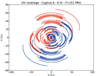
At any given time and frequency, one projected baseline samples one spatial frequency represented by one point in the (u, v) plane. With time, each (u, v) point sweeps the (u, v) plane, which enriches it with new samples (i.e. Earth rotation syn-thesis). Figure 1 presents the (u, v) coverage of one typical LOFAR observation integrated over six hours. Each track is as-sociated with one antenna pair, and its shape depends on the an-tenna configuration, the instrument latitude, and the direction of observation.

Fig. 1. Visibility coverage from a six-hour observation of Cygnus A (McKean et al. 2010). Visibilities are plotted in the Fourier space with the U (x-axis) andV (y-axis) being the spatial frequencies in wave-length unit,λ(here f =151 MHz,λ ≈2 m) determined by the base-line projection on the sky. Each (u, v) point (red) has its symmetric (−u,−v) point (blue) corresponding to the same baseline. The lines in-dicate (u, v) points where a visibility was recorded. The arcs are built from varying the baseline projections with the rotation of Earth during the observation.

We now discuss the different approaches that can be used to approach the true sky brightness from the measured visibilities, starting with the CLEAN method, before describing the method based on the sparsity of the measured signal.

2.2. CLEAN

For many years, deconvolution has been achieved through the CLEAN algorithm (Högbom 1974) and its variants (Clark 1980; Schwab 1984). CLEAN considers the dirty image to be con-structed from point sources convolved with the PSF; extended objects are decomposed as point sources as closely as possible. CLEAN operates directly on the dirty image (original versions like Högbom do) by locating the maximum of the image and iteratively subtracting a fraction of the dirty beam centred and scaled to the located maximum. The detected sources are in-dexed as CLEAN components to form a model image enriched by the successive subtraction steps. The source detection and subtraction continues until a threshold is reached on the resid-ual image (typically representing the background level), which is assumed to contain no remaining sources. The model image contains a pixel-wise description of the levels and locations of the detected sources. To remove the unphysically high spatial frequency components (associated with the pixel size) that are introduced by the CLEAN algorithm, the model image is usu-ally convolved by an elliptical Gaussian 2D fit of the centre of the dirty beam (which is the CLEAN beam) to provide a final an-gular resolution corresponding to that accessible by the interfer-ometer. The residual image, containing no other source, is added to the convolved CLEAN image to form the restored image and represents the noisy sky background.

This image can be described in the following manner:

I=M ∗C+R, (1)

where Iis the restored image, M is the model composed of CLEAN components,Cis the CLEAN beam,Ris the residual, and∗is the convolution operator.

The CLEAN method has several variants, one of which is Cotton-Schwab CLEAN (CoSch-CLEAN) fromSchwab(1984),

which was used for all experiments in this article. CLEAN can be described as a least-squares minimization that solves nor-mal equations and its variants that are usually split into ma-jor andminorcycles by combining a steepest-descent method (major cycle) and a greedy algorithm (minor cycle), which quickly calculates an approximate solution of the normal equations.

CoSch-CLEAN uses the steepest-descent method (during the major cycle) combined with a greedy algorithm (during the minor cycle) that calculates an approximate solution of the normal equations.

With LOFAR, the PSF varies over the FoV and is also dif-ficult to determine accurately because of instrumental DDEs (Sect. 2.5). Moreover, the sensitivity and variety of baseline s

brought by the instrument often limit the quality of the restored images using these methods.

2.3. Toward multi-resolution

The CLEAN method is well known to produce poor solu-tions when the image contains large-scale structures. Wakker & Schwarz (1988) introduced the concept of multi-resolution CLEAN (M-CLEAN) to alleviate difficulties occurring in CLEAN for extended sources. The M-CLEAN approach con-sists of building two intermediate images, the first one (called the smooth map) by smoothing the data to a lower resolution with a Gaussian function, and the second one (called the difference map) by subtracting the smoothed image from the original data. Both images are then processed separately. By using a standard CLEAN algorithm on them, the smoothed clean map and dif-ference clean map are obtained. The recombination of these two maps gives the clean map at the full resolution.

This algorithm may be viewed as an artificial recipe, but it has been shown that it is linked to wavelet analysis (Starck & Bijaoui 1991), leading to a wavelet CLEAN (W-CLEAN) method (Starck et al. 1994). Furthermore, in the W-CLEAN al-gorithm, the final solution was derived using a least-squares it-erative reconstruction algorithm applied to the set of wavelet coefficients detected by applying CLEAN on different wavelet scales. This can be interpreted as a debiased post-processing of the peak amplitudes found at the different scales. A positivity constraint on the wavelet coefficients was imposed during this iterative scheme by nullifying the negative coefficients.

However, these different CLEAN-based algorithms (here-after denoted x-CLEAN) have all shown to significantly improve the results over CLEAN when the image contains extended sources.

Other methods, based on a statistical Bayesian approach, have been developed to image extended emission (Junklewitz et al. 2013; Sutter et al. 2014) but were not included in the present work.

2.4. Compressed sensing and sparse recovery

Compressed sensing (Candès et al. 2006; Donoho 2006) is a sampling and compression theory based on the sparsity of an observed signal, which shows that under certain conditions, one can exactly recover a k-sparse signal (a signal for which only

kcoefficients have values different from zero out ofntotal co-efficients, wherek<n) fromm<nmeasurements. CS requires the data to be acquired through a random acquisition system, which is not the case in general. However, even if the CS theo-rem does not apply from a rigorous mathematical point of view, some links can still be considered between real life applications and CS. In astronomy, CS has already been studied in many ap-plications such as data transfer from satellites to Earth (Bobin et al. 2008;Barbey et al. 2011), 3D weak lensing (Leonard et al. 2012), next-generation spectroscopic instrument design (Ramos et al. 2011), and aperture synthesis. Indeed, there is a close re-lationship between CS principles and the aperture-synthesis im-age reconstruction problem, which was first addressed inWiaux et al.(2009a),Wenger et al.(2010),Li et al.(2011b) andCarrillo et al. (2012). Wide-field observations were subsequently stud-ied in McEwen & Wiaux (2011), and different antenna con-figurations (Fannjiang 2013) and non-coplanar effects (Wiaux et al. 2009a,b;Wolz et al. 2013) were analysed in a compressed-sensing framework. Aperture synthesis presents the three main ingredients that are fundamental in CS:

– Underdetermined problem: we have fewer measurements

(i.e. visibilities) than unknowns (i.e. pixel values of the reconstructed image).

– Sparsityof the signal: the signal to reconstruct can be

rep-resented with a small number of non-zero coefficients. For point source observations, the solution is even strictly sparse (in the Dirac domain) since it is only composed of a list of spikes. For extended objects, sparsity can be obtained in an-other representation space such as wavelets.

– Incoherence between the acquisition domain (i.e. Fourier

space) and the sparsity domain (e.g. wavelet space). Point sources, for instance, are localized in the pixel domain, but spread over a large domain of the visibility plane. Conversely, each visibility contains information about all sources in the FoV.

From the CS perspective, the best way to reconstruct an imageX from its visibilities is to use sparse recovery by solving the fol-lowing optimization problem:

minkXk_p subject to kV−AXk2₂< , (2) whereVis the measured visibility vector,Athe operator that

em-bodies the realistic acquisition of the sky brightness components (instrumental effects, DDE, etc.), andkzkp_p = P

i|zi|p. To rein-force the sparsity of the solution,pis positive but must be lower than or equal to 1. In particular, for p = 0, we derive the `₀

pseudo-norm that counts the number of non-zero entries in z. The first part of Eq. (2) enforces sparsity, the second part indi-cates that the reconstruction matches the visibilities within some

error. Most natural signals, however, are not exactly sparse but rather concentrated within a small set. Such signals are termed

compressibleorweakly sparse, in the sense that the sorted coef-ficient values decay quickly according to a power law. The faster the amplitudes of coefficients decay, the more compressible the signal is.

It is interesting to note that the CLEAN algorithm can be in-terpreted as amatching-pursuit algorithm(Lannes et al. 1997) that minimizes the`₀pseudo-norm of the sparse recovery prob-lem of Eq. (2), but recent progress in the field of numerical op-timization (see application with the SARA algorithm inCarrillo et al. 2014and references therein) allows us to have much faster algorithms. The sparsity model is extremely accurate for a field containing point sources, since the true sky can in this case be represented just by a list of spikes. This explains the very good performance of Högbom’s CLEAN for point sources recovery, and why astronomers still use it 40 years after it has been pub-lished. But CS provides a context in which we can understand the limitation of CLEAN for extended object reconstructions. The notion of sparsity in radio astronomy is not new and may be recognized in algorithms that apply a transform to the data. For example, extended objects are not sparse in the pixel basis, therefore sparse recovery algorithms cannot provide good solu-tions on this basis. Indeed, as depicted inWakker & Schwarz (1988) andStarck et al.(1994) with wavelets, representing the data in another domain where the solution is sparse was shown to be a good approach. More generally, we can assume that the solutionXcan be represented as the linear expansion

X=Φα=

t X

i=1

φ_iα_i, (3)

whereαare the synthesis coefficients of X,Φ = (φ₁, . . . , φ_t) is the dictionary whose columns aretelementary waveformsφ_i

also called atoms. The dictionary Φ is a b×t matrix whose columns are the normalized atoms (of size b), assumed here to be normalized to a unit`₂-norm, that is, ∀i ∈ [1,t],kφ_ik2₂ = PN

n=1|φi[n]|2 =1. The minimization problem of Eq. (2) can now be reformulated in two ways, the synthesis framework

min

α kαkp subject to kV−AΦαk

2

2< , (4)

and the analysis framework

min_α kΦtXk_p subject to kV−AXk2₂< . (5)

When the matrix Φ is orthogonal, both analysis and synthe-sis frameworks lead to the same solution, but the choice of the synthesis framework is generally the best if Xhas a clear and unambiguous representation inΦ.

2.5. Imaging with LOFAR

For a large multi-element digital interferometer such as LOFAR observing in a wide FoV, the small-field approximation is no longer valid, and the sampled data (represented by the opera-tor A) are no longer a discrete set of 2D Fourier components

of the sky. The instrumental (direction-independent) and natu-ral direction-dependent effects have to be taken into account for proper image reconstruction. These effects include

– the instrumental effects such as inter-station clock shifts, – the non-coplanar nature of the baselines (Cornwell & Perley

1992) and the effect of their projections (the sample visibility function has a non-zero third coordinate, i.e.w,0), – the anisotropic directivity of the phased-array beam

(Bhatnagar et al. 2008), and the non-trivial dipole projection effects with time and frequency,

– the sparsity in the sampling of the visibility function (i.e. the

limited number of baselines and the time/freq integration), and

– the effect of the interstellar- and interplanetary media, and

Earth’s ionosphere, on the incoming plane waves.

These effects can be modelled in the framework of the radio in-terferometry measurement equation (RIME; seeHamaker et al. 1996; Sault et al. 1996;Smirnov 2011 and following papers), which describes the relation between the sky and the four-polarization visibilities associated with each pair of antennas in a time-frequency bin. It can model all the DDE mentioned above, cumulated in 2×2Jonesmatrices that influence the elec-tric field and voltage measurements. One of the most basic ways to express a four-polarization visibility of one baseline using the RIME formalism is as follows (in a given time-frequency bin):

Vreal_pq =J−_p1V_pqmes(JH_q)−1, (6)

with

Vmes the four-polarization (XX, XY, YX, YY) measurement

matrix corrupted by the DDE,

Vtrue the true visibility matrix uncorrupted by the DDE, J_p the cumulatedJonesmatrix of antenna p, and

JH_q the Hermitian transpose (conjugated transpose) of the

cumu-latedJonesmatrix of antennaq.

The corrected visibilityVcorr_pq matrix can be expressed as a

four-dimensional vector (which also depends on the timet and fre-quencyν) as in Eq. (1) ofTasse et al.(2013),

Vec(Vcorr_pq )= Z

S(

Dt_qν,_,s∗⊗Dt_pν_,s)Vec(I_s)×e−2iπφ(u,v,w,s)ds, (7) whereI_sis the four-polarization sky,sthe pointing direction,⊗ the Kronecker product producing a 4×4 matrix (referred to as the Mueller matrix), Vec() the operator that transforms a 2×2 ma-trix into a four-dimensional vector,Dtqν,,s∗⊗Dtpν,s, the 4×4 Mueller

matrix, containing the accumulation of the direction-dependent terms and the array geometry (see details in Appendix A inTasse et al. 2013), andφ(u, v, w,s)= ul+vm+w(

√

1−l2−m2−1), the baseline and direction-dependent phase factor. Because the sky is described in terms of Stokes intensity (I,Q,U,V), and not in terms of the electric field value, the RIME is linear in its sky-term. By considering the total set of visibilities over base-lines, time, and frequency bins, and by including the measure-ment noise, we can therefore reduce Eq. (7) to

V=AI_s+, (8)

with

I_s the four-polarization sky;

A the transformation matrix from the sky to the visibilities,

including all DDE; and

the measurement noise.

The structure of matrixAand its connection to the RIME and

Jones formalism shown above is described in detail inTasse et al. (2012). The linear operatorA contains (i) the Fourier kernels

and the information on, (ii) the time-frequency-baseline depen-dence of the effective 2×2 Jones matrices, and (iii) the array configuration that is represented by the (u, v, w)-sampling over time and frequency. It is important to note that both (ii) and (iii) causeAto be non-unitary, which is a very important fact for the

work presented in this paper. In practice, it is virtually impos-sible to makeAexplicit, essentially because of itsN_vis×N_pixels dimension. Instead,AandATcan be applied to any sky or

vis-ibility vector respectively using A-projection(Bhatnagar et al. 2008;Tasse et al. 2013). To cope with the non-coplanar effect, theW-projectionalgorithm (Cornwell et al. 2008) is used to turn the 3D recorded visibilities into a 2D Fourier transform. In the scope of the LOFAR project and its data reduction pipeline, the AWimager (Tasse et al. 2013) program was developed for imaging the LOFAR data by taking into account both A- and W-projections. It is therefore of high interest to implement CS in this type of new-generation imagers.

2.6. Algorithm

To perform the sparse image reconstruction, we need to 1. select a minimization method to solve Eq. (4) or Eq. (5), 2. select a dictionaryΦ, and

3. select the parameter related to the minimization method. Several minimization methods have been used for aperture syn-thesis, the FISTA method (fast iterative shrinkage-thresholding algorithm inBeck & Teboulle 2009) inLi et al.(2011b),Wenger et al. (2010, 2013), and Hardy (2013), the OMP (orthogo-nal matching pursuit; Davis et al. 1997) in Fannjiang(2013), Douglas-Rachford splitting in Wiaux et al. (2009b), McEwen & Wiaux (2011) and Carrillo et al. (2012) or the SDMM simultaneous-direction method of multipliers inCombettes & Pesquet (2011) andCarrillo et al. (2014). In our experiments, we investigated mainly two algorithms, FISTA, and a recent algorithm proposed by V˜u (2013), which works in the analy-sis framework. As they were providing very similar results, we chose to report here results derived with the FISTA algorithm. Full details can be found inBeck & Teboulle (2009),Wenger et al.(2010), andStarck et al.(2010).

The convex optimization problem formulated in Eq. (4) can be recast in an augmented Lagrangian form with

min_α kV−AΦαk2₂+X j

λ_j|α_j|. (9)

The first part of Eq. (9) indicates that the reconstruction should match the data and the second term enforces sparsity (through controlling the regularization parameterλ_jat each scale jofΦ). The information about the errorin Eq. (2) is included inλ_j. The problem can then be solved using the FISTA algorithm (Beck & Teboulle 2009), following the implementation of algorithm1.

The final problem remains: choosing parameters that are needed to control the algorithm. Most minimization methods, using l0 and l1, have a single thresholding step, where coeffi

-cients in the dictionary have to be soft or hard-thresholded using a threshold value, which is a valueλ, common to projection inΦ

(unlike Eq. (9)) (seeStarck et al. 2010for more details on hard and soft thresholding). This parameter controls the trade-off be-tween the fidelity to the observed visibility and the sparsity of the reconstructed solution. InLi et al.(2011b) andWenger et al. (2013),λwas fixed to an arbitrary value, different for each ex-periment, and certainly after several tests. This approach may be problematic for real data where the true solution is not known.

Carrillo et al.(2014) addressed the constrained problem of Eq. (5) directly and the parameter is a bound on the`₂-norm data fidelity term, which is related explicitly to the noise level under the assumption that the noise is i.i.d.Gaussian. As the noise is generally not white, a whitening operator has to be applied first.

We propose in this paper another strategy, where the thresh-old is fixed only from the noise distribution at each wavelet scale j. Indeed, estimating a threshold from the residuals in a pixel basis is far from being optimal. On the one hand, the resid-ual is not necessarily of zero mean and the background level is not known, and, on the other hand, the signal can be at the noise level in the pixel basis, but much stronger in the wavelet basis.

This has two main advantages: the default threshold value should always give reasonable results, and it optimizes the prob-ability detection of faint objects. Indeed, an arbitrary threshold value could lead to many false detections in the case where the value is too low, and in contrast, many objects may be missed when the value is too high.

At thenth iteration of the FISTA algorithm, the residual im-ageRn_{is calculated by}

R(n)=µATV−AΦα(n), (10)

whereV are the measured visibilities,α(n) are the coefficients in the dictionary Φ of the solution at the nth iteration, and µ

is the FISTA relaxation parameter that depends on the matrix

F=AΦ(µmust verify 0< µ < _kF1_k). If the chosen dictionaryΦ

is the starlet or the curvelet transform, then the noise level can be estimated for each scale jof the residualR(n)_{using a reliable}

estimator such as the MAD (median of the absolute deviation):

σ(_jn) =MAD

α(_jR(n))

0.6745 , (11)

denotingα(R(n)₎

j the coefficients ofR(n)of the bandjin the dictio-naryΦ. The thresholdsλ_j(see Eq. (9)) are then different for each band, withλ_j =kσ_j, wherekfixes the probabilities of false de-tections. This provides the advantage of properly handling cor-related noise. The constant factor in Eq. (11) is derived from the quantile function of a normal distribution taken at probability 3/4 (Hoaglin et al. 1983).

Algorithm 1FISTA implementation

Require:

A dictionaryΦ. The implicit operatorA.

The original visibility dataV.

A detection level k.

The soft-thresholding operator: SoftThreshλ(α)=proxλ(α)=1−_|αλj

j|

+αj

1≤_j≤_N

1: Initializeα(0)_=0,t(0)₌₀

2: forn=0 toN_max−1do

3: β(n+1)_=x(n)_+µΦT_AT_(V−AΦα(n)₎

4: x(n+1)=SoftThreshµλ_jβ(n+1)

5: t(n+1)₌₍₁₊p

1+4(t(n)₎2_)/2

6: γ(n)_=(t(n)_−1)/t(n+1)

7: α(n+1)_=x(n)_+γ(n)_(x(n)_−x(n−₁₎₎ 8: end for

9: Return:imageΦα(Nmax).

3. Benchmarking of the sparse recovery

3.1. Benchmark data preparation

The performance of CS can be determined and compared to that of other imaging methods such as CoSch-CLEAN and MS-CLEAN. We used here three different LOFAR datasets (Table1) to compare CS and CLEAN-based algorithms in simulated and real situations.

We implemented CS by creating a new method in AWimager based on the current CoSch-CLEAN implementation. This new method serves as an entry point to the LOFAR imager to connect an external library (developed by the authors, see Sect.5.3) con-taining the dictionaries (wavelets and curvelets), transforms, and minimization methods described above. The CS cycle involves a continual passing of data back and forth between AWimager and the library (before and aftergridding,degriddingof the data, and applying theA-andW-projections). At step iin the CS cycle, AWimager performs the following operations:

– it takes as input an image reconstruction obtained at iteration i−1 (represented in the selected dictionary),

– it simulates the visibilities using the sameAoperator as for

CoSch-CLEAN (and performdegridding),

– it compares the simulated visibilities to the original ones, and – it passes the difference back to the dictionary using AT,

and performs a step of the CS minimization, thresholding, and produces a reconstructed image of iterationi.

The process stops if the maximum number of iterations is reached or if a convergence criterion (based on the noise of the residual) is met. The current implementation fits the cur-rent framework used by recent algorithms where the major cy-cle performs the CS operations (especially line 3 of Algo 1, which enables computing Eq. (10)). In the future, multiple steps of CS will be possible (in a minor cycle) to improve perfor-mance. AWimager outputs a similar set of files for both CoSch-CLEAN and CS (the restored, residual, model, and a PSF im-age). CLEAN output is a CLEAN-beam-convolved image; in the case of CS, the reconstructed image is the solution Φαn (Eq. (10)). The program user may choose to convolve the com-pressed sensing output with the CLEAN beam and/or add the residual image (see discussion in Sect.4.1). The CS residual isR(n)_{(Eq. (10)) at the last iteration of CS and is analogous to the}

Table 1.Summary information of the LOFAR datasets used in the present study.

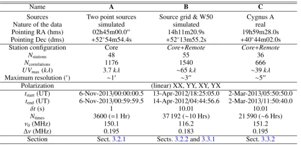
Name A B C

Sources Two point sources Source grid & W50 Cygnus A

Nature of the data simulated simulated real

Pointing RA (hms) 02h45m00.000 _{14h11m20.9s 19h59m28.0s} Pointing Dec (dms) +52◦_{54m54.4s +52}◦_{13m55.2s +40}◦_44m02.0s

Station configuration Core Core+Remote Core+Remote

Nstations 48 55 36

Ncorrelations 1176 1540 666

UVmax(kλ) 3.7kλ ∼65kλ ∼39kλ

Maximum resolution (0_{) ∼1}0 _∼300 _∼500

Polarization (linear) XX, YY, XY, YX

tstart(UT) 6-Nov-2013/00:00:00.5 13-Apr-2012/18:25:05.0 2-Mar-2013/05:50:50.0

tend(UT) 6-Nov-2013/00:59:59.5 14-Apr-2012/04:44:56.6 2-Mar-2013/11:50:40.0

δt(s) 1 10.01 10.01

Ntimes 3600 (=1 Hr) 37 192 (∼10 Hrs) 21 590 (∼6 Hrs)

ν0(MHz) 150.1 116.2 151.2

∆ν(MHz) 0.195 0.183 0.195

Section Sect.3.2.1 Sects.3.2.2and3.3.1 Sect.3.3.2

Notes. N_stationsandN_correlationsare the number of stations and the corresponding number of independent correlation measurements (computed as

Ncorrelations =Nstations(Nstations−1)/2+Nstations). Autocorrelations were systematically flagged before imaging.UVmaxis the largest radial distance

in the (u, v) plane that limits the maximum theoretical resolution of the instrument.tstart andtendobservation times are in Universal Time (UT),

providing a total number of time samples Ntimes at a time resolutionδt. We considered only one frequency channel covering a bandwidth∆ν

centred on the frequencyν₀. All three datasets come inmeasurements setsthat follow the NRAO standards. DatasetAhas been generated for a

one-hour synthetic zenith observation usingmkantandmakeMSroutines that are part of the LOFAR software package. DatasetBcomes from a

LOFAR commissioning observation and is filled with simulated data. DatasetCcontains actual calibrated data from a real LOFAR observation of

Cygnus A.

the meaning of some classical imager parameters are changed in the scope of the previous definitions: the gain in x-CLEAN con-trols the fraction of the PSF subtracted at each iteration. In CS, the gain is the relaxation parameterµof Eq. (10), which controls the convergence rate of the algorithm. The threshold value in x-CLEAN is a flux density value usually associated withntimes the level of noise measured (or expected) in the residuals (or in an source-free patch of the dirty image). Setting this threshold to zero would basically lead x-CLEAN to false detections from the background features. As discussed above in Sect.2.6, the CS thresholding parameter is defined for each or all bands in the chosen dictionary. The number of iterations for CoSch-CLEAN algorithm is set to a high value (>104_{to set an unrestrained}

con-vergence to the threshold). The number of iterations for CS can be set to an arbitrary value or be controlled by a convergence criterion.

The following figures of merit will measure the quality of the reconstruction using CS and CoSch-CLEAN methods:

– the total flux density computed in a region S around the

source,

– the residual image standard deviation (Std-dev) and root

mean square (rms) computed overS in the residual image

or over the full imageI,

– the error image and the mean square error (MSE) computed

overIwhen a model image is available, and

– the dynamic range (DR) defined as the ratio of the maximum

of the image to the residual Std-dev.

We here present different benchmark reconstructions arranged in increasing source complexity. In Sect.3.2, we reconstruct point sources in two typical situations implied by new-generation radio interferometers: at small scale, by reconstructing the image of two point sources at different angular separation (Sect.3.2.1), and at large scale, by reconstructing high-dynamic and wide-field images using a grid of point sources (Sect.3.2.2).

In Sect.3.3we monitor the reconstruction quality of extended emissions: from a simulated W50 observation (Sect.3.3.1) and a real LOFAR observation of Cygnus A (Sect.3.3.2).

3.2. Unresolved sources

3.2.1. Angular separation between two sources

When considering point sources, the x-CLEAN algorithms are usually the most frequently adapted reconstruction method. The first test is therefore to compare the performance of CS re-construction to that of CoSch-CLEAN for that simple type of source. We generated empty datasets (datasetAin Table1)

de-scribing a simulated one-hour LOFAR observation. We only used core LOFAR stations, since they are included in most LOFAR observation. This justifies the evaluation of the ground performance of CS on this array subset. The layout of the core stations is slightly elongated (∼10%,van Haarlem et al. 2013) in the north-south direction, providing a symmetric beam pattern to a direction close to zenith. In this dataset, we pointed the array to the local zenith, which will induce an a priori elongated beam pattern. The core stations in datasetAgive a highest resolution of

10_atν

0=150 MHz (in the HBA band). In addition, we restricted

the (u, v) coverage to the radial distances [rmin

(u,v),rmax(u,v)]=[0.1 kλ,

1.6 kλ] to artificially impose an angular resolution of∼20(which is effectively close to∼2.80_{as deduced from the PSF).}

We simulated two one-Jansky point sources at frequencyν₀. With this simple sky model, we used the blackboard self-cal pro-gram (BBS;Pandey et al. 2009) to fill the LOFAR dataset with simulated visibilities. One source is located at the phase cen-tre, the second is located at varying angular distancesδθranging from 1000 _{up to 5}0_{. As a consequence, we span various}

δθ=30’’

δθ=1’

δθ=2’ δθ=1’30’’

δθ=2’30’’

δθ=3’ δθ=1’15’’

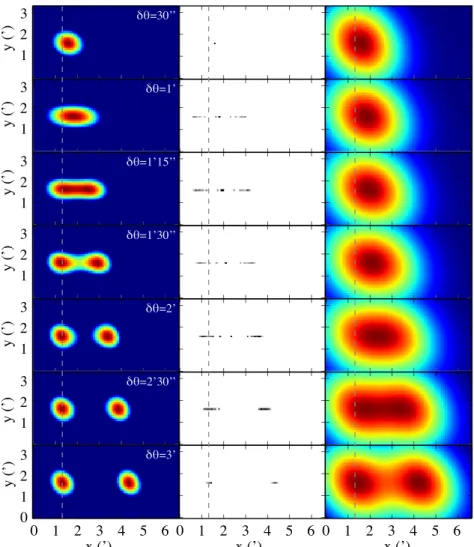
Fig. 2.Resulting reconstructed CS image (left column), CoSch-CLEAN model (middle column), and convolved (right column) images obtained from a simulation of two point sources with different angular separationδθfrom 3000_{to 3}0_{by steps of 30}00_{(from top to bottom) plus theδθ=1}0₁₅00 case. Thethird columnwas obtained by convolving the CLEAN components (middle column) with the CLEAN beam ofFWHM3.180_×2.550_{. The} effective separation of the two sources, after imaging by the different methods, occurs at smaller angular separation with CS (betweenδθ=10_and δθ =10₁₅00_{) than with CoSch-CLEAN (betweenδθ=2}0_andδθ=20₃₀00_{). The unambiguous separation of the two sources was obtained within} few pixel errors, starting fromδθ=10₃₀00_{for CS andδθ =3}0_{for CoSch-CLEAN. Each cropped image was originally of size 512×512 pixels} of 500_{. The (u, v) coverage has been restricted to the [0.1 kλ,1.6 kλ] domain to enforce an artificial resolution of∼2}0_{. The colour map scales are} normalized to the maximum of each image, but colour bars were not represented for clarity. The contrast of the CLEAN components (middle column) was enhanced to ease their visibility. The grey vertical dash line marks the true position of the source located at the phase centre of the dataset.

ii) partially resolved; or iii) unambiguously resolved. As we are close to the phase centre, the effects mentioned in Sect.2.5are negligible (which will no longer be the case in Sect.3.2.2). For different angular separations, we injected Gaussian noise on the visibilities to obtain effective signal-to-noise ratio (S/N) levels of∼3,∼9,∼16, and∼2000 (noise-free case) in the image.

We used the original CoSch-CLEAN and our CS method im-plemented in AWimager, which serves here as a common test-ing environment for this study. We performed 104_{iterations for}

the CoSch-CLEAN and 200 iterations for CS. As different lev-els of noise were simulated, we set thekparameter (Eq. (11)) to three times the noise level. We used for both algorithms the (u, v)-truncated dataset as described above and produced 512 ×512 pixel images at 500 pixel resolution. We imposed a

natural weighting scheme to improve the S/N of the resulting images.

Figure2 illustrates the results obtained with the noise-free dataset: the CS reconstruction (left column), the CoSch-CLEAN model image (middle column), and the correspondingconvolved

image (right column). The rows correspond to seven values of

angular separationδθfrom 3000 _{to 3}0 _{by steps of 30}00 _{and the} δθ =10₁₅00 _{case. For the CS reconstruction, there is no model}

image in the CLEAN sense because the output of CS is di-rectly the best representation of the true sky at a finite resolu-tion (similar to the comparison of models in Li et al. 2011b). Different angular separation criteria can be chosen. One can ap-ply the Rayleigh criterion based on the separation of two (pixel) CLEAN components on the model image or use source-finders on reconstructed images (see below). Here (and hereafter), the CLEAN beam, setting the highest angular resolution of CLEAN deconvolved images, has a size of 3.180_×2.550_{(major×minor}

axes). In the CoSch-CLEAN model image, whenδθ is small, only one group of CLEAN components is detected at the mean position of the two sources. Starting fromδθ=10₃₀00_{, additional}

CLEAN components are being detected on thewingsof the main component, but are located correctly on the source position. Withδθincreasing, the amplitudes of these side CLEAN compo-nents increase and contribute in the resulting elongated shape on the convolved CLEAN image. Starting fromδθ=20₃₀00_{, the two}

of components around the correct position. The position uncer-tainty of these two sources is still high (∼3000_{). For separations}

larger thanδθ=30_{, the astrometric and flux density errors start}

to decrease. In the regime where CoSch-CLEAN cannot unam-biguously resolve the two sources, the features present in the model images (the central components as well as the wing com-ponents) cannot be associated with real sources. In the scope of this method, an exploitable image with limited resolution can only be obtained after convolving with the CLEAN beam.

With CS, we directly obtain the best estimate of the sky, as shown in the reconstructed image in the left column of Fig. 2. In the partially resolved regime, we also note that the elongation of the source size occurs atδθ=10_{. We note that the two point}

sources are resolved at lower angular separation (δθ ∼ 10₁₅00₎

than for CoSch-CLEAN. An elliptical fit of the FWHM of the sources gives the source size, which can be seen as the ef-fective CS convolution beam. In this case, its dimensions are 1.550_×1.090_{, representing a beam of cross-section approximately}

1.390_{, which is smaller than that of the CLEAN beam. In}

addi-tion to the improved angular separability, the CS reconstructed sources are also correctly located in the image (e.g. the central source lies close to the vertical mark in Fig. 2forδθ ≤10₃₀00₎

as compared to the CoSch-CLEAN model image, where the CLEAN components are only correctly positioned starting from

δθ ≤ 20₃₀00_{. In the noise-free case, by using exactly the same}

dataset and imaging parameters, these results suggest that CS is able to recover information on the true sky beyond the theoretical resolution limit (which is constant in this dataset). Because there is always a non-zero level of noise in the calibrated interfero-metric data, we tested the reliability of this characteristic against the image S/N by using the different noisy datasets mentioned above.

To compute the effective angular separability of the sources using CoSch-CLEAN and CS, we used the LOFAR pyBDSM3 package (python blob detection and source measurement), which consists of island detection, fitting, and characterization of all structures in the image. We defined a detection threshold so that no other artefact could be detected as a source in the images because we only focused on the two simulated point sources. We used the same set of detection parameters for CoSch-CLEAN and CS images.

At a specific S/N level, the limit value of angular separation at which two distinct sources can be distinguished by the source finders gives an estimate of the separability angle of the sources and therefore of the effective resolution that limits the typical size of genuine physical features. The CoSch-CLEAN beam and the effective CS beam are not circular, therefore the absolute effective angular resolution may depend on the orientation of these beams with respect to the direction joining the two sources. To have a measure that is independent of this direction, it is probably better to compute the ratio between the beam ellipti-cal parameters obtained with CoSch-CLEAN and that obtained with CS.

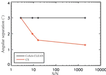
Using an appropriate sampling ofδθand noise levels, we can build a graph of this effective resolution deduced from the sepa-rability of the two sources for different S/N levels. We present in Fig.3the resulting curves obtained with CoSch-CLEAN (black) and CS (red). For each S/N we derived the effective improve-ment brought by CS by noting the angleδθ_minat which the two sources are separated. On the one hand, the CoSch-CLEAN sep-arability has a limited dependence on the S/N, which makes it a

3 _{Seehttp://www.lofar.org/wiki/doku.php}

for more information.

Angular separation (’)

S/N

CoSch-CLEAN CS

Fig. 3.Values ofδθ_minof source separability as a function of the S/N for CS (red curve) and CoSch-CLEAN (black curve). In the moderate (S/N≥ 5) and high S/N regimes, the resulting source separability is improved by a factor 1.3 to<_∼2.

stable and reliable algorithm for detecting point sources in var-ious S/N regimes. On other hand, CS behaves differently. At a high S/N regime, the separability values outperforms that of CoSch-CLEAN by a factor of 2–3 in the [10, 2000] S/N range. When the S/N decreases, the separability of CS tends to that of CoSch-CLEAN.

In terms of astrometric error, the detected point source loca-tions can be compared to the (α, δ) coordinates of the input sky model (where the sources were placed at pixel centres). The rel-ative position errors do not exceed 10_{for CS and 3}0_{for CLEAN}

for all the different noise levels.

In addition to the angular separability and astrometric errors, we inspected the flux density of the source.

Naturally, the flux density error of the reconstructed sources is affected by the level of the background noise and scales with the S/N. It is found to be 3% in the low-noise regime and up to 25% in the high-noise regime for CS and 3% to 23% for CoSch-CLEAN.

From this perspective, it appears that CS provides results that are almost as good as the results by CLEAN by default, and pro-vides an improved angular separability with high and moderate S/N data. The low astrometric and flux density error confirm the superior resolution capability of CS, which suggests the possi-bility of dramatically improved angular resolution of extended emission from poorly sampled interferometric data.

3.2.2. Wide-field imaging of a grid of sources

Interferometry imaging at low frequencies implies a larger FoV because of the size of the LOFAR station analogue beam. By us-ing AWimager, which deals with wide FoV (Tasse et al. 2013), we checked the ability of CoSch-CLEAN and CS to recover the correct flux density of point sources that are away from the phase centre. We simulated a 10×10 grid of point sources over a re-gion of 8◦_×8◦_{around the phase centre. Their flux densities range}

from 1 to 104_{Jy. We used BBS to fill datasetBby enabling the}

simulation of the beam (for theA-projection). TheW-projection

only depends on the layout of the interferometer, which is in-cluded in the dataset. Noise was injected into the dataset to pro-vide an rms value of 10−4_{(so∼1 Jy) relative to the peak of the}

Right Ascension (J2000)

D

ec

li

na

ti

on (J

2000)

+50°

Jy/

be

am

+52° +54° +56°

+48°

13h50m00s 14h0m00s

10m00s 20m00s

30m00s

9000

7500

6000

4500

3000

1500

0

-1500

Fig. 4.Dirty image derived from a set of 100 simulated point sources with flux density ranging from 1 to 104 _{Jy. Simulated visibilities are}

generated with datasetB. Some sources are not yet visible because of

the dynamic of the source and the noise level.

density and the potential residual distortions over the field with-out overlapping of the source. While this arrangement is un-realistic, we can still monitor the astrometric and flux density accuracy versus the radial distance from the phase centre. We ap-plied CoSch-CLEAN and CS to the simulated dataset containing the grid. The dirty image generated from visibilities is shown in Fig.4.

We used 1024×1024 pixel images with a pixel size of 2800

and the full (u, v) coverage of dataset B was used for

imag-ing, giving an effective angular resolution of∼300_{. For}

CoSch-CLEAN, we used 108_{iterations and for CS, we used 200}

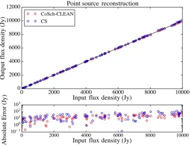
itera-tions. With CS, the sources were reconstructed with the starlet dictionary. We report in Fig. 5 the output integrated flux den-sity of all detected sources in the reconstructed images against the input flux densities of the sky model point sources. A sound reconstruction should put every source on the first bisector. We again used pyBDSM to perform the source detection and charac-terization (including the 2D elliptical Gaussian fit of the source, position of the Gaussian barycentre, and photometry along with providing respective errors). The error bars of each point were obtained directly from the photometry and are negligible given the low level of the background noise. However, these error bars do not include the bias of poorly reconstructed sources.

For the CS reconstructed image, the effective source size is reduced to smaller patches with a few pixels each around the sources (comparable to the CLEAN model, only constituting a collection of pixels). The flux is more efficiently gathered around the source position, resulting in an increase of all pixel size val-ues in the CS images (in Jy/beam). The resulting source size was 3.20_×3.70_{(i.e. the dimension of the CLEAN beam) for}

CoSch-CLEAN and between∼3000₋₁0_{(1–2 pixels) for CS. This result}

corroborates that of the previous study. The superior resolution here yields an improvement of a factor of 3 to 6 of the source size compared to the size of the CLEAN beam, using exactly the same dataset (and weighting) for the two methods.

The flux density rms error was derived from the resid-ual images and accounts for 3.6 Jy/beam Std-dev of CS and

0 2000 4000 6000 8000 10000

Input flux density (Jy) 0

2000 4000 6000 8000 10000 12000

O

u

tp

u

t

fl

u

x

d

en

si

ty

(J

y

)

Point source reconstruction

CoSch-CLEAN CS

0 2000 4000 6000 8000 10000

Input flux density (Jy)

10− 1

100

101

102

103

A

b

so

lu

te

E

rr

o

r

(J

y

)

Fig. 5.Top: total flux density reconstruction for a set of point sources (Fig.4) with original flux density spanning over 4 orders of magni-tude with the original flux density (x-axis) vs. the recovered flux density (y-axis).Bottom: scatter plot of the absolute the error for each source. The recovered flux densities for CoSch-CLEAN (red) and CS (blue) are represented on a linear scale, whereas the absolute error is on a logarithmic scale for clarity. Perfect reconstruction lies along the black line. The output flux density values and errors are similar with both CoSch-CLEAN and CS.

1.7 Jy/beam Std-dev for CoSch-CLEAN. The error bars are not reported in the plot for clarity. The relative error (compared to the input flux density of each source) is not larger than 10% in most cases for both CoSch-CLEAN and CS. The flux density er-ror slightly increases with the source flux density, as depicted by the scatter plot represented in a log-scale in Fig.5(bottom).

As a result of the many strong sources, CoSch-CLEAN and CS were unable to reconstruct some faintest sources barely above the background level. CoSch-CLEAN presents slightly better performances for reconstructing correct flux densities with a lower error (the mean absolute error is 19 Jy for CLEAN and 29 Jy for CS). Nevertheless, CS led to the detection of more faint sources that were missed by CoSch-CLEAN, but with a larger error on their flux density values. In spite of its improved angular resolution and its detection capability, CS provides a larger Std-dev (3.6 Jy/beam) on the residual image than CoSch-CLEAN (1.7 Jy/beam). This could be an effect of the thresholding taking place in CS or the choice of the dictionary, which is not perfectly fitted to represent point sources.

We did not note any particular dependence on the radial dis-tance from the phase centre for either CoSch-CLEAN or CS. This suggest that theA- and W-projections in AWimager cor-rectly prevented a radial dependence of the flux, the astrometric error, and the source distortion (the last two being at the scale of one pixel). This tell us that the CS method is effectively com-patible with the RIME framework. Moreover, x-CLEAN algo-rithms remain competitive with CS because the spatial exten-sion of wavelet atoms is not as efficient as Dirac atoms (pixel) in representing single point sources.

3.3. Extended sources

0 512 1024 X

0 512 1024

Y

0 0.25 0.5 0.75 1

m

Jy

/pi

x

el

14h05m 10m 15m 20m

RA (J2000) +51°

D

ec

(J

2000)

0.4 0.8 1.2 1.6

Jy/

be

am

+52° +53°

0.6 1.0 1.4

0.2

0

Fig. 6.Left: original 1.4 GHz radio image fromDubner et al.(1998) (pixel size=6.7500_{, ang. resolution=55}00_{),middle: prepared input model} image scaled to the approximate total flux density of 230 Jy (1024×1024 with pixel size of 13.500_{), andrightthe dirty image obtained with} datasetB. All emission falling outside the extended emission of W50 was set to zero, but point sources inside W50 were kept in the simulation.

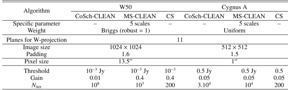
Table 2.Relevant imaging parameters used by AWImager for CoSch-CLEAN, MS-CLEAN, and CS, for the two extended objects.

Algorithm W50 Cygnus A

CoSch-CLEAN MS-CLEAN CS CoSch-CLEAN MS-CLEAN CS

Specific parameter – 5 scales – – 5 scales –

Weight Briggs (robust=1) Uniform

Planes for W-projection 11

Image size 1024×1024 512×512

Padding 1.6 1.5

Pixel size 13.500 ₁00

Threshold 10−_{3Jy 10}−_{3Jy 10}−_{3 0.5 Jy 0.5 Jy 0.5}

Gain 0.01 0.4 0.4 0.05 0.05 0.05

Niter 108 103 200 3.104 104 200

Notes.For MS-CLEAN, we have used scales at [0,10,30,70,100] pixels for W50, and [0,2,5,10,15] pixels for Cygnus A.

dictionary for the CS reconstruction to ensure the best sparsity of the signal. We first study a simulation of W50 (Sect. 3.3.1) and then discuss the results of CS on a real LOFAR observation of Cygnus A (Sect.3.3.2).

3.3.1. Simulated observation: the W50 nebula

The W50 nebula (hosting the SS 433 microquasar) is an ex-tended supernova remnant of large dimension (∼2◦ _{× ∼1}◦_{) with}

internal filamentous structuring that makes it proper for bench-marking CS and CLEAN-based algorithms. First, we used the W50 brightness image from Dubner et al. (1998) (Fig.6 left). This image at 1.4 GHz is rich in information at various angu-lar scales down to an anguangu-lar resolution of∼5500 _{(the image at}

327.5 MHz, taken with the VLA in the D configuration, was also available, but no structures smaller than 700 _{are resolved).}

We assumed that the higher spatial frequency features also emit in the LOFAR band (see W50 observed with LOFAR HBA in Broderick et al. in prep. and previous work). We focused on the central extended emission by removing part of the extraneous foreground and background features. We set the flux scale of the total model image to match a total flux density of ∼250 Jy at 116 MHz as interpolated fromDubner et al.(1998). Second, we used thepredict task of AWimager to convert the input model to visibilities in datasetB. No artificial DDEs were inserted in

the simulation but A-projectionandW-projectionwere enabled for all runs. DatasetBprovides a theoretical angular resolution

of∼300_{, which is higher than the 55}00_{of the original image. We}

therefore expect to have good results for all three methods. The

predict step samples the image at the resolution of dataset B.

Given the size of W50, the simulated field is 3.8◦_×3.8◦_{. Third,}

artificial Gaussian noise was added to the simulated visibilities and has an effective rms of 3×10−4_{of the peak of the dirty} noise-freeimage (corresponding DR ∼4000). We reconstructed im-ages using three methods: CoSch-CLEAN, MS-CLEAN, and CS in AWimager. MS-CLEAN was imported from the LWimager, the standard LOFAR imager, superseded by AWimager.

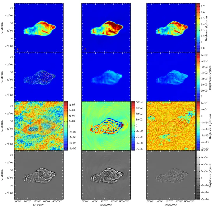
With the input model image, we computed the error image and inspected the residual images to track the effective angular resolution and the convergence of the methods. Table2gathers all imaging parameters (as well as for Cygnus A). We compare in Fig.7the outputs of CoSch-CLEAN (left column), MS-CLEAN (central column), and CS (right column). From top to bottom we present the reconstructed image, the model, the residual age, and the error image. The figure of merit from these im-ages is gathered in Table3. The total reconstructed flux densities over the source are 229.2 Jy, 229.4 Jy, and 229.7 Jy for CoSch-CLEAN, MS-CoSch-CLEAN, and CS. These values are extremely close to the 230 Jy of the model, which verifies that all three methods conserve the total flux density. This fact is a basic requirement that any new imaging method should verify.

+ 51°₀₀ 30 + 52°₀₀ 30 + 53°₀₀ 30 D ec (J 2 0 0 0 ) 0.0 0.1 0.2 0.3 0.4 0.5 0.6 0.7 B ri g h tn es s (J y /b ea m )

+ 51°₀₀ 30 + 52°₀₀ 30 + 53°₀₀ 30 D ec (J 2 0 0 0 ) 0 3e-03 5e-03 7e-03 1e-02 1e-02 2e-02 2e-02 B ri g h tn es s (J y /p ix el )

+ 51°₀₀ 30 + 52°₀₀ 30 + 53°₀₀ 30 D ec (J 2 0 0 0 ) -1e-03 -8e-04 -5e-04 -3e-04 0 3e-04 5e-04 8e-04 1e-03 -6e-02 -4e-02 -3e-02 -1e-02 0 1e-02 3e-02 4e-02 6e-02 -2e-03 -2e-03 -1e-03 -8e-04 -4e-04 0 4e-04 8e-04 B ri g h tn es s (J y /b ea m )

14h₀₄m₀₀s 08m₀₀s 12m₀₀s 16m₀₀s 20m₀₀s

RA (J2000) + 51°₀₀

30 + 52°₀₀ 30 + 53°₀₀ 30 D ec (J 2 0 0 0 )

14h₀₄m₀₀s 08m₀₀s 12m₀₀s 16m₀₀s 20m₀₀s

RA (J2000)

14h₀₄m₀₀s 08m₀₀s 12m₀₀s 16m₀₀s 20m₀₀s

RA (J2000) -6e-04 -4e-04 -2e-04 0 2e-04 4e-04 6e-04 8e-04 B ri g h tn es s (J y /p ix el )

Fig. 7.Reconstructed images of W50 from the simulated LOFAR observation (datasetB) using CoSch-CLEAN (left column), MS-CLEAN (middle

column), and CS (right column).From top to bottom: the restored (in Jy/beam), the model (in Jy/pixel), the residual, and the error images. The CS restored and model images only differ by their scaling (the former is in Jy/beam using the beam area of the CoSch-CLEAN beam, the latter is in Jy/pixel). The colour scales of the images are different for each row, as indicated by the colour bar on the right. The residual images are displayed with their respective colour bar. The CS reconstruction contains high spatial frequency information restored from the dataset. The effective angular resolution of the CS image (10_{) is close to that of the original input image (55}00_{). In addition, the error image shows a closer proximity between CS} and the original input image.

caused by an inappropriate thresholding when the background residual level is reached, the algorithm then start to get signal from the background noise. In comparison, we also used the MS-CLEAN method of LWimager and obtained equivalently poor results. MS-CLEAN results might be improvable with additional controls and masks, but we chose a straightforward imaging (as our algorithm) to highlight the robustness of our algorithm with a limited number of user controls. Moreover, the implementation of MS-CLEAN in AWimager is still experimental and needs to be more extensively validated. This method is known to usually improve the representation of extended sources.

The restoring beam was 2.80_×2.40_{for CoSch-CLEAN and}

2.80_×3.30 _{for MS-CLEAN. The CS image is visually sharper}

than the other two and contains high-frequency features that were recovered during the imaging. From the typical point source size in the CS image, the effective angular resolution was ∼10× ∼10, nearly equal to the 5500 original resolution, and rep-resents an improvement of almost a factor 2.5–3 over x-CLEAN images.

Table 3.Statistical results obtained from applying CoSch-CLEAN, MS-CLEAN, and CS to all the datasetsA,B, andC.

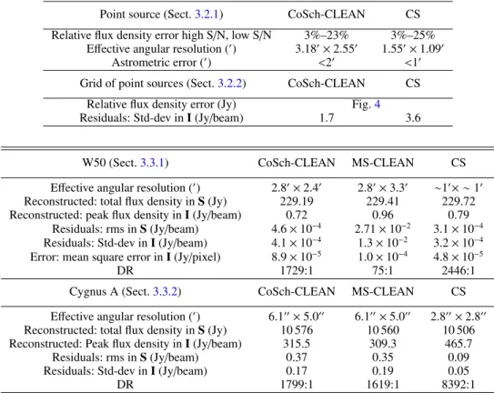
Point source (Sect.3.2.1) CoSch-CLEAN CS Relative flux density error high S/N, low S/N 3%–23% 3%–25%

Effective angular resolution (0_{) 3.18}0_×2.550 _1.550_×1.090 Astrometric error (0_{) <2}0 _<10 Grid of point sources (Sect.3.2.2) CoSch-CLEAN CS

Relative flux density error (Jy) Fig.4 Residuals: Std-dev inI(Jy/beam) 1.7 3.6

W50 (Sect.3.3.1) CoSch-CLEAN MS-CLEAN CS

Effective angular resolution (0_{) 2.8}0_×2.40 _2.80_×3.30 _∼10_{× ∼1}0 Reconstructed: total flux density inS(Jy) 229.19 229.41 229.72

Reconstructed: peak flux density inI(Jy/beam) 0.72 0.96 0.79

Residuals: rms inS(Jy/beam) 4.6×10−4 _2.71×10−2 _3.1×10−4 Residuals: Std-dev inI(Jy/beam) 4.1×10−_{4 1.3×10}−_{2 3.2×10}−₄ Error: mean square error inI(Jy/pixel) 8.9×10−5 _1.0×10−4 _4.8×10−5

DR 1729:1 75:1 2446:1

Cygnus A (Sect.3.3.2) CoSch-CLEAN MS-CLEAN CS Effective angular resolution (0_{) 6.1}00_×5.000 _6.100_×5.000 _2.800_×2.800 Reconstructed: total flux density inS(Jy) 10 576 10 560 10 506

Reconstructed: Peak flux density inI(Jy/beam) 315.5 309.3 465.7

Residuals: rms inS(Jy/beam) 0.37 0.35 0.09

Residuals: Std-dev inI(Jy/beam) 0.17 0.19 0.05

DR 1799:1 1619:1 8392:1

Notes.The statistics are defined in the text and appear when applicable.Imeans that the quantity has been evaluated on the entire image,Sin a

defined region of the image (typically around the source).

image only differ by the residual image that was added to the lat-ter. CS tends to concentrate even more the flux of point sources around the source (see Sect.3.2.1), and the starlet dictionary is able to correctly represent the extended emission.

Any vestigial structures in the residual image show a lower rate of convergence, which might be due to an insufficient number of iterations (which is currently not the case for the x-CLEAN algorithms), or a limitation due to the imaging method itself. In our case, the CoSch-CLEAN image, supposed to perform better with point sources than with extended emis-sion, presents a lower residual Std-dev level (4.1×10−4Jy/beam) than that of MS-CLEAN (1.3×10−2_{Jy/beam) in the present}

sit-uation. However, the CS residual Std-dev level is slightly bet-ter (3.2×10−4_{Jy/beam) across the image. The error images are}

shown in the last row of Fig.7and are the difference between the restored image (converted to Jy/pixel) with the initial full reso-lution input image (also in Jy/pixel). The input image was not degraded by convolution to match a particular resolution. From the different error images, CS visually provides the lowest error. The high-resolution features were partly restored by the CS re-construction. The CS algorithm has the lowest mean square error value over the image (4.8×10−5_{Jy/pixel), which represents an}

improvement of a factor∼2 compared to that of present CoSch-CLEAN and MS-CoSch-CLEAN reconstructed images.

3.3.2. Real LOFAR observation: the Cygnus A radio galaxy

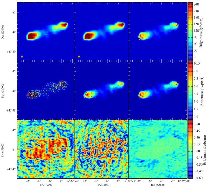
Cygnus A (3C 405) is one of the most powerful galaxies ob-servable in the radio domain. It serves as a good test case for benchmarking our method: it contains extended emission, origi-nating from two main radio lobes (representing a projected size

of∼20_×10_{) as well as compact emissions at the extremities of}

each lobe (the hotspots A and B in the western lobe and hotspot D in the eastern lobe, as labelled in Hargrave & Ryle 1974). Cygnus A has recently been observed by LOFAR during its com-missioning phase (McKean et al. 2010), but has also been long observed in the past at low frequencies for instrumental calibra-tion or science (e.g.Lazio et al. 2006 and references therein, who observed Cygnus at 74 MHz and 327 MHz with the VLA). We used a real calibrated LOFAR dataset (C) at 151 MHz

con-taining real noisy measurements. The data were previously cali-brated on the Perley-Butler (2010) absolute flux scale (McKean et al. 2010).

Similar imaging parameters were used (Table2). With the FoV being relatively small and the source being the dominant source in the dataset, the DDEs were expected to be low. In Fig. 8, we show the same output images as in Sect. 3.3.1. However, we do not have an input model image to compute the error image. From left to the right, columns are the reconstructed image with CoSch-CLEAN, MS-CLEAN, and CS. From top to bottom, the rows present the reconstructed images in Jy/beam, the model images in Jy/pixel, and the residual image.

All the three methods rendered a proper image of the emis-sion, given the extremely good quality of the data and the strong source brightness. The CoSch-CLEAN image shows residual high-frequency structures that lead to distortions of the source. These artefacts mainly come from CLEAN components col-lected from the noise background residual image. With MS-CLEAN, we obtained a similar brightness distribution to that in McKean et al.(2010). The restoring beam size was 6.100_×5.000