OCEANOGRAPHIC AND GEOMAGNETIC INFLUENCES
ON SEA TURTLE MIGRATIONS
Nathan Freeman Putman
A dissertation submitted to the faculty of the University of North Carolina at Chapel Hill in
partial fulfillment of the requirements for the degree of Doctor of Philosophy in the
Department of Biology (Evolution, Ecology, and Organismal Biology).
Chapel Hill
2011
Approved by:
Dr. Kenneth J. Lohmann
Dr. John M. Bane
Dr. John F. Bruno
Dr. William M. Kier
© 2011
Abstract
NATHAN F. PUTMAN: Oceanographic and Geomagnetic Influences on Sea Turtle Migration (Under the direction of Dr. Kenneth J. Lohmann)
The research presented here explores the migratory behavior of sea turtles from behavioral, ecological, and evolutionary perspectives. Turtles display long-distance migratory movements at all stages of their lives; as hatchlings they migrate offshore from nesting beaches, as juveniles they navigate oceanic gyres, and as adults they move between foraging and reproductive grounds. For each of these migrations I examine how behavioral processes mediate large-scale biogeographic patterns.
Analyses revealed a relationship between sea turtle nest abundance and offshore oceanic conditions. A disproportionate number of nests were deposited on beaches near ocean currents that facilitate the successful migration of hatchling turtles. This nesting pattern may persist through time because turtles return to nest near their natal beaches; thus, areas that produce the most surviving hatchlings and juveniles might also have the highest number of adults returning to nest.
Laboratory experiments demonstrated that young turtles are capable of extracting latitudinal and longitudinal information from the earth’s magnetic field to assess their position along their open ocean migration. Computer simulations indicated that even limited swimming in response to these magnetic cues exerts considerable influence on the open-ocean distribution of turtles. Specifically, magnetic navigation behavior appears to increase the number of turtles that encounter
navigation in turtles, combined with geomagnetic and ocean circulation models, provided the first quantitative insight into how environmental conditions select for the evolution of this behavior.
Finally, geomagnetic models were used to explore the long-standing mystery of how female turtles return to their natal beach after dispersing thousands of kilometers over a decade or more. Analyses indicate that a simple strategy of imprinting on the magnetic field of the natal site and using this information to return at maturity can account for the known homing precision of several different species of sea turtles. Moreover, the predictions from this hypothesis are consistent with the
ACKNOWLEDGEMENTS
I am exceptionally grateful to those who have supported me through my time in graduate school. Most notable is my advisor Ken Lohmann who has served as a constant source of inspiration for research ideas, guidance, and funding. I am particularly indebted to my conversations with Matt Füxjager in my first year of graduate study which helped plot the course of my research in a number of ways. Katrin Stapput, Courtney Endres, Cathy
TABLE OF CONTENTS
LIST OF TABLES ...ix
LIST OF FIGURES ...x
Chapter
I.
INTRODUCTION ...1
II.
THE OFFSHORE MIGRATION OF HATCHLING SEA TURTLES ...5
Is the geographic distribution of nesting in the Kemp’s ridley sea turtle
shaped by the migratory needs of offspring? ...7
Sea turtle nesting distributions and oceanographic constraints on
hatchling migration ...23
III.
THE PELAGIC MIGRATION OF JUVENILE SEA TURTLES ...37
Exploring the geospatial organization of hatchling loggerhead sea
turtles’ magnetic map ...39
Longitude perception and bicoordinate magnetic maps in sea turtles ...50
Orientation responses of loggerhead sea turtles to magnetic fields in
the North Atlantic ...60
Transoceanic migratory dispersal of young sea turtles: a little
navigation goes a long way ...67
The evolution of magnetic way-mark navigation in sea turtles ...81
IV.
NATAL HOMING AND THE MAGNETIC IMPRINTING
HYPOTHESIS ...95
Island finding: magnetic imprinting, bicoordinate navigation, and
secular variation at eight major green turtle nesting sites ...108
Ecological implications of natal homing by magnetic imprinting in
loggerhead sea turtles ...123
V.
CONCLUSIONS...141
List of Tables
Table
2.1 Mean percentage of simulated turtles that reach pelagic habitat within four days and recruit to
foraging grounds within two years. ... 13
2.2 Relative migratory success by nesting region. ... 14
2.3 Mean percentages of simulated turtles that recruit to foraging grounds when starting from different nesting regions. ... 15
2.4 Regional scale data from loggerhead nesting range along the southeast U.SA ... 26
2.5 Local (county) scale data from loggerhead nesting range along Florida, U.S.A. ... 27
2.6 Results of regression analyses predicting nest density as a function of each area’s distance to the GSS and latitude ... 31
3.1 Information on the magnetic treatments presented to hatchling loggerheads ... 46
3.2 Information on the magnetic treatments presented to hatchling loggerheads. ... 52
3.3 Information on the magnetic treatments presented to hatchling loggerheads. ... 63
3.4 Parameters of the behavioral scenarios modeled ... 73
3.5 Experimental parameters and orientation responses of turtles to magnetic fields that occur in the North Atlantic ... 83
3.6 Secular variation and oceanic factors associated with each magnetic point. ... 85
3.7 AIC metrics used in model selection and results of multiple regression analyses... 87
3.8 Regression coefficients and significance levels of variables contributing to the best model ... 87
4.1. Modeled navigational errors for Kemp’s ridleys assuming time to maturity at 10 and 15 years, imprinting on either inclination angle or total field intensity based on BGS from 1600-1900... 100
4.2. Modeled navigational errors for Kemp’s ridleys assuming time to maturity at 10 and 15 years, imprinting on either inclination angle or total field intensity based on IGRF-10 1600-1900. ... 100
4.3. Average rate of field change (1900 - 2010) at various coastal locations where sea turtles, salmon, and elephant seals return to reproduce. ... 103
4.4 Mean field movement from 1900-2010 over 25 year periods at 8 green turtle rookeries ... 121
4.5 Mean field movement from 1900-2010 over 5 year periods at 8 green turtle rookeries ... 122
List of Figures
Figure
2.1 Map of the study region. ... 11
2.2 Graph of the mean percentage of simulated Kemp’s ridley hatchlings from each nesting
region that reach pelagic habitat (water deeper than 200 m) within four days. ... 12
2.3 Graph of the mean percentage of simulated Kemp’s ridley hatchlings that recruit to coastal foraging grounds within 2 years.. ... 13
2.4 Bar graph showing estimated nest abundance for each nesting region. ... 14
2.5 Surface current velocity in the Gulf of Mexico based on HYCOM output.. ... 18
2.6 Graph of the mean percentage of simulated Kemp’s ridley hatchlings from Rancho Nuevo that recruit to the five regions of Fig. 2.1... 20
2.7 Map of loggerhead nesting range along the southeastern U.S. coastline ... 29
2.8 Graphs of loggerhead nest density plotted against distance from each nesting area to the GSS ... 32
2.9 The partitioning of variance of nest density of southeastern U.S. loggerhead sea turtles ... 35
3.1 Representation of the Earth’s magnetic field.. ... 38
3.2 Hypothetical geospatial organization of the magnetic map of loggerhead sea turtles.. ... 41
3.3 Schematic of experimental apparatus, including the orientation arena, magnetic coil
structure, and data acquisition system. ... 43
3.4 Circle diagrams representing the magnetic treatments turtles were exposed to.. ... 47
3.5 Schematic of North Atlantic Subtropical Gyre and orientation of hatchling loggerheads tested in a magnetic field from the west side of the Atlantic near Puerto Rico and in a field from the east side of the Atlantic near the Cape Verde Islands. ... 53
3.6 Maps of magnetic elements in the North Atlantic Ocean.. ... 56
3.7 Map illustrating the feasibility of turtles using unique combinations of magnetic inclination and intensity to distinguish among longitudes at the same latitude but on opposite sides of the
Atlantic. ... 57
3.8 Map of the North Atlantic Subtropical Gyre... 64
3.9 Map of possible dispersal routes of juvenile loggerheads migrating from southeast Florida, U.S.A. ... 72
3.10 Mean percentages of turtles entering the South Atlantic Bight, Mid-Atlantic Bight, latitudes higher than 46° N, the region of the Bahamas and Sargasso Sea and Azores within 5 years. ... 74
3.11 The relative difference between the predicted distribution of turtles based on passive
3.12 Percent of turtles reaching the Azores from 0.5 - 5.0 years (mean of means) for different
behavioral scenarios. ... 76
3.13 Graph showing the mean percent increase from passive drift for turtles reaching the Azores after first entering suboptimal oceanic regions when simulated with navigation behavior ... 77
3.14 Maps of secular variation for three magnetic points in the North Atlantic.. ... 89
3.15 Mean surface temperature across the North Atlantic.. ... 91
3.16 Mean surface velocity across the North Atlantic.. ... 92
3.17 Example of variability in current directions at two locations in the North Atlantic.. ... 93
4.1 Map of the Gulf of Mexico indicating the nesting area of the Kemp’s ridley turtle and the locations to which turtles would hypothetically return under two simple magnetic imprinting strategies ... 101
4.2 Bar graph showing hypothetical navigational errors for turtles that imprinted on inclination angle or intensity at specific points in time and returned to the coastal location marked by the same magnetic value 10 or 15 years later ... 102
4.3 Location of islands used in this study ... 111
4.4 Mean navigational errors estimated for turtles returning to the magnetic target after a 25 year absence from the natal island and mean size of magnetic target. ... 113
4.5 Mean navigational errors estimated for turtles returning to the magnetic target after a 5 year absence from the natal island and mean size of magnetic target... 114
4.6 Direction of island from the magnetic target ... 118
4.7 Hypothetical strategy for locating an island with a single magnetic coordinate ... 119
4.8 Maps of the eight major loggerhead nesting beaches where simulations of natal homing via magnetic imprinting were modeled. ... 126
4.9 The graph shows results from simulations between 1900 and 2010 for turtles leaving the natal site and returning at maturity and after 5 years ... 130
4.10 Linear regressions of loggerhead nest abundance vs. the change in inclination angle over a twenty year period. ... 134
4.11 Map of Florida, USA and inclination angle ... 137
4.12 Temporal variation in nest abundance explained by change in inclination angle vs. the magnitude of mean field drift ... 139
CHAPTER 1
INTRODUCTION
The movement of organisms is a fundamental component of nearly all ecological and evolutionary processes, providing insights into phenomena at all levels of biological organization from physiology and behavior of individuals to broad-scale biogeographic patterns (Nathan 2008; Nathan et al. 2008). For example, the amount of gene flow among populations appears to be largely controlled by the movement capacity of a species (i.e. vagility). Species with a greater capacity for movement typically have increased gene flow among populations whereas less vagile species tend to have more structured populations (McCracken et al. 1994; Hamrick & Godt 1996). As a result, over evolutionary timescales, organisms with low capacity for movement may be more likely to evolve adaptations to localized selective agents (e.g. the environment, specific competitors, certain predators, or a specialized food source) which could eventually lead to speciation. In contrast, panmixia
(random mating throughout a species’ range) is likely to occur for species with high movement capacity and local adaptations may be less likely to evolve (Avise 2009).
organism movement is that it is inherently directional. Thus, detailed examination of the
environmental and biological factors that promote, impede, and directionally bias the movement of organisms is likely to provide the optimal framework for studying ecological and evolutionary phenomena (Alerstam et al. 2003; Holyoak et al. 2008; Bowlin et al. 2010).
In studying the complexities of organism movement, long-distance migratory animals have proven to be excellent model systems (Alerstam 2006; Åkesson & Hedenström 2007; Nathan 2008). The clear directionality of migration can often be highly amenable to hypothesis generation and experimentation with regard to the factors that animals use to assess their position and orient their movements. Additionally, the extensive distances traveled by migrants help to highlight how movement is a crucial component of energy acquisition, reproduction, and the evolution of traits associated with these tasks (Alerstam et al. 2003; Åkesson & Hedenström 2007). Likewise, the specialized adaptations in behavior and physiology that permit migrants to successfully navigate across heterogeneous landscapes provide opportunities to explore how the movement of individual organisms varies depending on environmental conditions.
In my dissertation I address unresolved issues fundamental to animal movement, particularly in long-distance migrants. Among these are the following: (1) the navigational mechanisms that guide long-distance movements; (2) how the mechanisms used influence the path of animals and errors in navigation; (3) how environmental constraints on migration influence the evolution of navigation strategies; and (4) the ecological and evolutionary implications of migrations for populations. I explore these questions by studying diverse aspects of the migratory behavior in sea turtles. The broad and multidisciplinary approach I present here is unified by the goal of describing how the directed movement of individuals shapes the biogeographic patterns exhibited in sea turtle species.
My dissertation is organized around three types of migrations that sea turtles undertake: (1) the offshore migration of hatchlings from the natal site; (2) the pelagic foraging phase of juveniles; and (3) the return to the natal site by adults for reproduction. Each migration is the focus of a single chapter that is further subdivided into sections that represent studies providing insight into the
navigational mechanisms utilized by sea turtles during migration, aspects of the physical environment that shape turtle movement, and the population-level consequences arising from the interaction between sea turtles’ migratory behavior and environmental factors.
and spatiotemporal patterns in sea turtle nesting. The final chapter provides a broader context for these studies by highlighting the implications of my research to the field of movement ecology, as well as potential applications to conservation and management initiatives in sea turtles.
CHAPTER 2
THE OFFSHORE MIGRATION OF HATCHLING SEA TURTLES
Historically, the nesting beach has been the most studied habitat of sea turtles, and yet no research has been carried out to address what factors influence spatial variation in nest density across the reproductive grounds of any sea turtle species. Instead, research to determine the factors that influence the spatial distribution of sea turtle nesting has largely focused on environmental parameters that ensure successful incubation (e.g. appropriate temperature, substrate, moisture, etc.) at individual nesting beaches (Carthy et al. 2003; Miller et al. 2003). However, the data from these studies are often conflicting and an unambiguous picture of what drives the spatial distribution of nesting has yet to emerge at the scale of the nest site (Miller et al. 2003). It is therefore difficult to extrapolate from these fine-scale studies what influences variation in nesting abundance across the nesting range of any sea turtle species.
Extensive monitoring of sea turtle nesting shows that some areas consistently have higher numbers of nests than others (Ehrhart et al. 2003). In this chapter I provide the first conceptual model that accounts for the variation in nest density across the nesting range of two sea turtle species. While there are certainly many factors that contribute to the observed spatial pattern in marine turtle nesting, I show that characteristics of the ocean rather than the beach are likely to exert the greatest influence the nesting distribution.
behavior to escape intense predation that occurs over the continental shelf and to access distant high-productivity foraging grounds (Wyneken & Salmon 1992).
Is the geographic distribution of nesting in the Kemp’s ridley sea turtle
shaped by the migratory needs of offspring?
Summary
Across the geographic area that a species uses for reproduction, the density of breeding individuals is typically highest in locations where ecological factors promote reproductive success. For migratory animals, fitness depends, in part, on producing offspring that migrate successfully to habitats suitable for the next life-history stage. Thus, natural selection might favor reproduction in locations with conditions that facilitate the migration of offspring. To investigate this concept, the Kemp’s ridley sea turtle (Lepidochelys kempii) was studied to determine whether coastal areas with the highest levels of nesting have particularly favorable conditions for hatchling migration. The passive drift of young Kemp’s ridley turtles was modeled from seven nesting regions within the Gulf of Mexico to foraging grounds using the particle-tracking program ICHTHYOP and surface-current output from HYCOM (HYbrid Coordinate Ocean Model). Results revealed that geographic regions with conditions that facilitate successful migration to foraging grounds typically have higher abundance of nests than regions where oceanographic conditions are less favorable and successful migration is difficult for hatchlings. Thus, these findings are consistent with the hypothesis that, for the Kemp’s ridley turtle and perhaps for other migrants, patterns of abundance across the breeding range are shaped in part by conditions that promote or impede the successful migration of offspring.
Introduction
adults return to reproduce in their natal area (Bowen and Karl 2007; Lohmann et al., 2008), the locations that produce the greatest number of surviving individuals may, over time, come to have higher abundance due to the higher reproductive success of individuals that breed in such places. Patterns of distribution within breeding areas of migratory species might thus remain relatively stable over considerable periods of time.
This conceptual framework is explored in a migratory sea turtle, the Kemp’s ridley (Lepidochelys
kempii). This species nests mostly within a limited area of coastline on the east coast of Mexico near
Rancho Nuevo (23.2° N, 97.5° W), but scattered nesting also occurs from Texas, U.S.A. to southern Campeche, Mexico (Márquez 1994; Plotkin 2007) (Fig. 2.1). Hatchlings enter the sea and
immediately migrate offshore to pelagic waters, thereby escaping intense nearshore predation that occurs over the continental shelf (Wyneken and Salmon 1992). After a period ranging from several months to two years, turtles enter coastal foraging grounds (Zug et al. 1997, Zimmerman 1998; TEWG 2000), typically either in the Gulf of Mexico between Texas and southwestern Florida or in locations along the eastern U.S. coast from Florida to Nova Scotia (Carr 1957; Hildebrand 1982; Ogren 1989; Metz 2004; Geis et al. 2005). In these coastal areas, turtles forage for benthic
invertebrates such as the blue crab Callinectes sapidus (Shaver 1991; Werner 1994; Metz 2004). At 10-15 years of age, Kemp’s ridleys return to their natal region to mate and nest (Caillouete 1995; Zug et al. 1997), after which they migrate back to distant foraging grounds and repeat this cycle every 1-3 years throughout their lives (TEWG 2000).
the regions within the Gulf of Mexico where most Kemp’s ridleys nest have oceanographic conditions that are particularly favorable for facilitating the migration of young turtles from their natal beach to suitable coastal foraging grounds.
Methods
A simple model was developed to investigate whether differences in relative abundance of nests across the Kemp’s ridley nesting range can potentially be explained by how well different regions facilitate young turtles’ migration to their foraging grounds. The Kemp’s ridley nesting range was partitioned into seven regions: Texas (29°N, 94.3°W - 26°N, 96.55°W); North of Rancho Nuevo (25.75°N, 96.55°W - 24.25°N, 97.1°W); Rancho Nuevo (23.75°N, 97.3°W - 22.9°N, 97.3°W); South of Rancho Nuevo (22.8°N, 97.2°W - 21.75°N, 96.95°W); Veracruz (21.3°N, 96.8°W - 18.95°N, 94.5°W); South Campeche (18.9°N, 94.5°W - 19.45°N, 91.5°W); and North Campeche (19.4°N, 91.4°W - 21°N, 90.95°W) (Fig. 2.1).
To simulate the movement of young turtles through the ocean Global HYCOM (HYbrid Coordinate Ocean Model) surface currents (0 m depth) were used (Bleck 2002). This model has a spatial resolution of 0.08° (~5-7 km) and a temporal resolution of one day. Young turtles were simulated using the particle tracking program ICHTHYOP v. 2 (Lett et al. 2008). Simulated turtles were released in a zone 45-55 km offshore from each of the seven regions, a distance from shore that hatchling sea turtles are known to reach (Witherington 2002). One thousand simulated hatchlings were released at one-week intervals starting June 1 and continuing through July 20 (eight total release events per year, per region). Turtles were allowed to drift passively for up to two years. HYCOM output is available from 2004-2009; therefore two years of dispersal for four yearly cohorts of hatchlings (2004 –2007) were simulated. The simulation for each year-class was replicated ten times. Thus, the dispersal of 320,000 turtles was simulated from each of the seven nesting regions.
Canada between Florida and Nova Scotia (Carr 1957; Hildebrand 1982; Ogren 1989; Metz 2004; Geis et al. 2005). Some reports also suggest that young Kemp’s ridley might recruit to coastal areas in Campeche Bay, Mexico (Márquez 1994). For purposes of analysis, the foraging grounds of juveniles were partitioned into five coastal areas: (1) Campeche Bay; (2) Texas; (3) Louisiana – West Florida; (4) East Florida – North Carolina; and (5) Virginia – Nova Scotia. These areas extended from the coast across the continental shelf, to a depth of 200 m (Fig. 2.1). Because very young turtles are unlikely to survive in nearshore waters due to intense predation (Collard and Ogren 1990), turtles could only recruit to a coastal region after reaching a minimum age of six months (Zimmerman 1998, TEWG 2000). Additionally, a turtle had to remain in a region for three days before it was considered to have recruited there. Each turtle could only recruit to one region.
How well a region facilitates migration of young sea turtles is likely determined by (1) how quickly hatchlings get offshore (thereby minimizing time spent over the continental shelf, where the risk of predation is probably highest) and (2) the percentage of hatchlings that reach suitable foraging grounds. Thus, for each region, measurements were taken of the percentage of simulated hatchlings that reached pelagic waters (i.e., water with a depth > 200 m) within four days, as well as the percentage of turtles that reached known coastal foraging grounds (Fig. 2.1) within two years.
were not significantly different, but region 1 was significantly different from region 3, then regions 1 and 2 shared the same rank and region 3 was given that rank plus 0.5. The mean of both ranks was taken as the relative “migratory quality” of each region.
An additional analysis was carried out to assess patterns of movement and the geographic locations where juvenile Kemp’s ridley turtles recruited to coastal feeding grounds. For simulated turtles starting from each of the seven nesting regions, the mean percentage of turtles that reached each of the five foraging areas (defined in Fig. 2.1 and in the text) was determined.
Results
The mean number of simulated turtles that reached pelagic habitat within four days was significantly different among nesting regions (ANOVA two-factor with replication, F6, 252 = 130927, p < 0.0001). Over the four years simulated, pelagic recruitment success was highest for Veracruz, Rancho Nuevo and South Campeche. Paired t-tests revealed no significant difference between Veracruz and Rancho Nuevo (p = 0.072) or Rancho Nuevo and South Campeche (p = 0.489), although pelagic recruitment success was significantly higher for turtles from Veracruz than for turtles from South Campeche (p < 0.0001). From other regions, approximately an order of magnitude fewer simulated Kemp’s ridley reached pelagic waters within four days (Table 2.1, Fig. 2.2).
The mean number of turtles reaching foraging grounds within two years was significantly different among nesting regions (ANOVA two-factor with replication, F6, 252 = 16890, p < 0.0001). The regions with the highest percentage of turtles entering foraging grounds were South Campeche, Rancho Nuevo, and Veracruz. Paired t-tests revealed no significant difference between South Campeche and Rancho Nuevo (p = 0.105). However, turtles from South Campeche and Rancho Nuevo had significantly higher recruitment success than did turtles from Veracruz (p < 0.001, p = 0.023 respectively). All other regions had significantly lower recruitment success than these three (p < 0.001 for each comparison) (Table 2.1, Fig. 2.3).
Figure 2.2 Graph of the mean
Table 2.1 Mean percentage of simulated turtles that reach pelagic habitat within four days and recruit to foraging grounds within two years. Results are given for each year and for each nesting region and are based on ten replicates for each year (see Methods for details). Numbers in italics indicate the 95% C.I. for the mean.
Year Texas North RN
Rancho Nuevo
South
RN Veracruz
South Campeche North Campeche 2004 Pelagic Habitat 1.58% (0.08%) 12.94% (0.23%) 35.06% (0.28%) 8.09% (0.19%) 57.84% (0.45%) 52.15% (0.33%) 0.0% (0.0%) 2004 Foraging Grounds 3.55% (0.22%) 7.87% (0.18%) 22.53% (0.22%) 2.93% (0.17%) 14.65% (0.22%) 18.79% (0.43%) 8.35% (0.18%) 2005 Pelagic Habitat 2.93% (0.10%) 4.98% (0.17%) 58.60% (0.33%) 1.43% (0.12%) 50.20% (0.51%) 23.66% (0.32%) 0.0% (0.0%) 2005 Foraging Grounds 3.74% (0.19%) 11.27% (0.28%) 18.19% (0.30) 3.55% (0.17%) 17.50% (0.22%) 20.62% (0.30%) 14.27% (0.30%) 2006 Pelagic Habitat 1.86% (0.11%) 0.0% (0.0%) 0.0% (0.0%) 0.0% (0.0%) 36.55% (0.34%) 41.62% (0.35%) 0.0% (0.0%) 2006 Foraging Grounds 8.72% (0.20%) 0.09% (0.03%) 1.73% (0.09%) 0.55% (0.07%) 11.11% (0.27%) 31.27% (0.41%) 12.74% (0.22%) 2007 Pelagic Habitat 2.37% (0.07%) 4.07% (0.19%) 65.67% (0.39%) 7.78% (0.24%) 42.83% (0.47%) 26.51% (0.33%) 0.0% (0.0%) 2007 Foraging Grounds 17.02% (0.32%) 15.17% (0.25%) 34.56% (0.20%) 7.29% (0.17%) 20.51% (0.25%) 22.82% (0.25%) 7.98% (0.22%) Mean Pelagic Habitat 2.18% (0.17%) 5.50% (1.52%) 39.83% (8.30%) 4.33% (1.18%) 46.86% (2.59%) 35.99% (3.75%) 0.0% (0.0%) Mean Foraging Grounds 8.26% (1.77%) 8.60% (1.80%) 19.25% (3.81%) 3.58% (0.78%) 15.94% (1.13%) 23.37% (1.55%) 10.83% (0.89%)
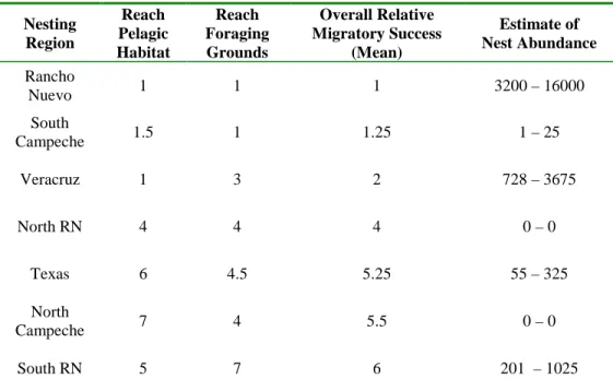
Paired t-tests for the two migratory metrics (mean recruitment to pelagic habitat and coastal foraging grounds) and subsequent ranking of the seven nesting regions revealed that, for the four years modeled, Rancho Nuevo best facilitated the migration of the turtles. Rancho Nuevo was followed closely by South Campeche and Veracruz whereas North of Rancho Nuevo, Texas, North Campeche, and South of Rancho Nuevo were considerably worse in facilitating the migration (Table 2.2, Fig. 2.4).
Table 2.2 Relative migratory success by nesting region. Nesting regions are ranked relative to one another from high (1) to low (7) for each metric used to measure migratory success (percentage of turtles that reach pelagic habitat within four days and percentage of turtles that reach foraging grounds within two years). See text for details. The overall migratory rank of a region (determined by the mean of ranks) is in the fourth column. The final column provides the range of recent estimates of nest abundance (Read et al. 2010).
Nesting Region
Reach Pelagic Habitat
Reach Foraging Grounds
Overall Relative Migratory Success
(Mean)
Estimate of Nest Abundance
Rancho
Nuevo 1 1 1 3200 – 16000
South
Campeche 1.5 1 1.25 1 – 25
Veracruz 1 3 2 728 – 3675
North RN 4 4 4 0 – 0
Texas 6 4.5 5.25 55 – 325
North
Campeche 7 4 5.5 0 – 0
South RN 5 7 6 201 – 1025
Nesting regions had significant differences in the percentage of simulated Kemp’s ridley that recruited to the five defined foraging grounds (ANOVA two-factor with replication F4, 180 > 20000, p < 0.0001, for each nesting region). Out of all the simulated turtles that reached coastal foraging grounds (regardless of the location from which they started), the largest percentage recruited to coastal Texas (52.8 %), followed by Louisiana to W Florida (33.9 %), East Florida to North Carolina (12.9 %), Virginia to Nova Scotia (0.3 %), and Campeche Bay (<0.1 %). Table 2.3 provides the distribution of Kemp’s ridley recruits by nesting region.
Table 2.3 Mean percentages of simulated turtles that recruit to foraging grounds (columns) when starting from different nesting regions (rows). Means are based on simulations of four two-year periods (2004-2006; 2005-2007; 2006-2008; 2007-2009). Italicized numbers below indicate the 95% C.I. of the mean.
Nesting Region Texas Campeche
Bay LA – WFL EFL – NC
VA – Nova Scotia
Texas 5.140%
(1.500%) 0.005% (0.002%) 2.462% (0.373%) 0.636% (0.109) 0.016% (0.005%)
North RN 4.207%
(1.387%) 0.007% (0.003%) 2.781% (0.526%) 1.568% (0.482%) 0.038% (0.014%)
Rancho Nuevo 9.163% (2.790%) 0.016% (0.007%) 6.955% (1.240%) 3.037% (0.822%) 0.082% (0.025%)
South RN 1.877%
(0.655%) 0.001% (0.001%) 1.153% (0.187%) 0.528% (0.149%) 0.014% (0.006%)
Veracruz 8.096% (1.330%) 0.024% (0.009%) 5.465% (0.254%) 2.311% (0.612%) 0.046% (0.015%) South Campeche 12.669% (1.510%) 0.025% (0.009%) 8.161% (0.866%) 2.461% (0.527%) 0.058% (0.021%) North Campeche 6.253 (0.595%) 0.008% (0.005%) 3.508% (0.382%) 1.042% (0.274%) 0.023% (0.008%) Discussion
Models of oceanic circulation indicate that the migratory success of young turtles (the percentage of simulated turtles that quickly reach pelagic waters and also successfully reach foraging grounds) is highly variable across the Kemp’s ridley nesting range. Thus, from the standpoint of the ease with which young turtles are likely to complete their initial migration, the different regions of coastline are not equal.
conditions are favorable to the migration of hatchlings. The lack of standardized nest counts across the Kemp’s ridley nesting range precludes a detailed quantitative analysis, but recent estimates of the numbers of nests in different geographic areas (Read et al. 2010) suggest that, in general, nesting is highest at locations with conditions that most effectively facilitate successful migration, whereas less nesting occurs in regions where successful migration is more difficult (Fig. 2.4, Table 2.2). The findings are consistent with the hypothesis that patterns of nest abundance are influenced, at least in part, by oceanographic conditions that facilitate or impede the migration of young turtles. Moreover, patterns of nest distribution are likely to be sustained over time by the natal homing of adults,
inasmuch as nesting locations that facilitate the migration of young turtles to foraging grounds lead to increased survival of juveniles, which in turn leads to increased numbers of adults returning to the same nesting locations where they themselves began life.
Departures from the Predicted Pattern
Although oceanographic factors that facilitate migration may influence which nesting beaches are used, such factors by themselves are clearly insufficient to account fully for the present distribution of nesting in the Kemp’s ridley. In at least two cases (South Campeche and South of Rancho Nuevo), the number of nests reported deviated from the predicted pattern. Interestingly, however, it is possible that special circumstances explain each departure.
According to the metrics used in the model, South Campeche possesses oceanographic conditions that facilitate both the offshore migration of young turtles and their subsequent movement to coastal foraging grounds. Nevertheless, this area has very little nesting. Evidence suggests, however, that the lack of nesting is a relatively recent development, and that a large population once existed in this area before it was nearly extirpated due to intense harvesting of adults and eggs by humans (Márquez 1994; Guzmán et al. 2007).
predictions, few turtles should nest there. However, this area attracts the third highest number of nesting turtles. Clearly, additional or alternative factors must be important in shaping the pattern of nesting.
South of Rancho Nuevo is immediately adjacent to the largest nesting assemblage at Rancho Nuevo. An interesting speculation is that some nesting in this region might result from navigational errors by adult Kemp’s ridley turtles attempting to return to Rancho Nuevo. If so, then it is unclear why the errors are asymmetrical, inasmuch as considerably more nesting occurs in the South of Rancho Nuevo area than in the North of Rancho Nuevo area. Conceivably, asymmetrical
navigational errors might occur if turtles imprint on the magnetic field of the natal beach and then return to a slightly different location because the earth’s field has shifted in their absence (Lohmann et al. 2008a). Indeed, geomagnetic modeling suggests that, over the past 400 years, adult Kemp’s ridley turtles attempting to relocate Rancho Nuevo after a 10-15 year absence would arrive at Rancho Nuevo or slightly to the south if they imprinted on magnetic inclination angle (Putman and Lohmann 2008). Whether this occurs is not known.
Yearly variation in migratory success
In some of the geographic regions, migratory success was relatively constant across the time period of the analysis, but in other areas, it varied considerably from year to year (Table 2.1). In general, the nesting regions of Texas, Veracruz, South Campeche, and North Campeche had relatively constant percentages of recruitment for each of the four cohorts of hatchlings, both in terms of
For instance, averaged over the four periods simulated, the regions of Rancho Nuevo, South Campeche, and Veracruz all had similar high recruitment success to pelagic habitat and to foraging grounds. However, recruitment success in different periods was not constant. During certain periods of limited duration, oceanic currents at Rancho Nuevo transported exceedingly large numbers of young turtles offshore and subsequently to foraging grounds (Table 2.1). The most favorable conditions occurred during the 2007-2009 simulation. During the 2007 hatching period, there was a well developed anti-cyclonic eddy directly offshore of Rancho Nuevo, resulting in strong offshore movement of simulated hatchlings (Fig. 2.5). In contrast, there was an unusually poor period for recruitment to pelagic habitat and foraging grounds during the 2006-2008 simulation. The
oceanographic cause seems to have been a northward shift of a semi-permanent westward flowing current (Fig. 2.5). Typically, this current bifurcates to the south of Rancho Nuevo, resulting in north-northeastward flowing water transporting hatchlings offshore, but in 2006, this westward flow was centered at Rancho Nuevo, directly opposing offshore progress of turtles. In the model, this led to very few turtles reaching pelagic habitat because they were washed shoreward; the limited number of turtles reaching the open sea in turn led to fewer turtles recruiting to foraging grounds. It is possible that the frequency of oceanic conditions which facilitate or impede the offshore migration of
hatchlings might be an important but previously overlooked factor in the population dynamics of the Kemp’s ridley.
Modeled Distribution of Juvenile Kemp’s Ridley
The vast majority of Kemp’s ridley hatchlings originate at Rancho Nuevo (Márquez 1994; Plotkin 2007; Read et al. 2010). Discussion will therefore be limited to the simulation involving this nesting region. Because the defined coastal foraging grounds (Fig. 2.1) vary in length from 490-1650 km, measures of recruitment are standardized by calculating, for each of the five regions, the
percentage of turtles that recruited per 100 km of continental shelf length (Fig. 2.6).
Simulated turtles from Rancho Nuevo most commonly reached the coastal waters of Texas (9.2% of the total simulated turtles; 0.99% per 100 km of continental shelf). Fewer simulated turtles reached other known foraging areas, including: Louisiana-West Florida (7.0% of the total; 0.58% per 100 km); East Florida-North Carolina (3.0% of the total; 0.20% per 100 km); Virginia-Nova Scotia (0.08% of total; 0.005% per 100 km); and Campeche Bay (0.02% of total; 0.003% per 100 km).
These results are consistent with a descriptive study by Collard and Ogren (1990), which indicated that turtles embarking on their migration from Rancho Nuevo would typically be transported offshore and to coastal locations along the Gulf and Atlantic coasts of the U.S. These findings also appear consistent with the numerous accounts of juvenile Kemp’s ridley turtles inhabiting coastal waters of the southeastern U.S. (Carr 1957; Hildebrand 1982; Ogren 1989; Metz 2004; Geis et al. 2005). That ocean currents do not carry many Kemp’s ridley from Rancho Nuevo to
Campeche Bay may also help explain why no juvenile turtles have been found there, despite seemingly suitable habitat (Carr 1980; Márquez 1994).
Implications for Conservation
These findings are consistent with the hypothesis that patterns of nest abundance for sea turtles are strongly influenced by oceanic conditions that promote or impede the successful migration of young turtles. Such considerations have important implications for conservation efforts. For example, in a program begun about 30 years ago, approximately 24,000 Kemp’s ridley eggs and hatchlings were relocated from Rancho Nuevo to Texas (Márquez et al. 2003, Shaver and Wibbels 2007). The goal was to establish a second area where the turtles nest and thus avert the possibility of a population collapse. Although there has been much debate on the merits of this project, it is now apparent that at least some of these “head-started” turtles are returning to Texas to nest (Shaver and Wibbels 2007). The findings here, however, suggest that conditions off the Texas coast are relatively poor in terms of facilitating the migration of young turtles (Figs. 2.2, 2.3), which might make it difficult for a large population to become established. Although protecting Kemp’s ridley nesting across Texas is certainly important to aid in the conservation of this critically endangered species, without concurrent protection of the Rancho Nuevo and Veracruz regions (which allow for high migratory success and presently have high abundance of nests), the efforts in Texas may be of limited value.
Additionally, attempts to predict the impact of climate change on sea-turtles’ nesting distribution may benefit from a consideration of the migratory requirements of young sea turtles, integrated with previously studied factors such as beach temperatures and coastal substrate.
Special Thanks
I am grateful to P. Verley for assistance with ICHTHYOP, to T. Kristiansen for help formatting HYCOM output, and to R. Márquez and T. Wibbels for providing information on Kemp’s ridley distributions. I appreciate E.M. Putman, E. Seney, and J. Wyneken for offering useful feedback on earlier versions of the manuscript.
Citation
Sea turtle nesting distributions and oceanographic constraints on hatchling migration Summary
Patterns of abundance across a species’ reproductive range are influenced by ecological and environmental factors that affect the survival of offspring. For marine animals whose offspring must migrate long distances, natural selection may favor reproduction in areas near ocean currents that facilitate migratory movements. Similarly, selection may act against the use of potential reproductive areas from which offspring have difficulty emigrating. As a first step toward
investigating this conceptual framework loggerhead sea turtle (Caretta caretta) nest abundance along the southeastern U.S. coast was analyzed as a function of distance to the Gulf Stream System (GSS), the ocean current to which hatchlings in this region migrate. Results indicate that nest density increases as distance to the GSS decreases. Distance to the GSS can account for at least 90% of spatial variation in regional nest density. Even at smaller spatial scales, where local beach conditions presumably exert strong effects, at least 38% of the variance is explained by distance from the GSS. These findings suggest that proximity to favorable ocean currents strongly influences sea turtle nesting distributions. Similar factors may influence patterns of abundance across the reproductive ranges of diverse marine animals such as penguins, eels, salmon, and seals.
Introduction
Numerous animals range over vast expanses of land or sea but reproduce only in
For animals that migrate long distances, additional environmental factors might also influence survival. For example, the offspring of some fish, shorebirds, penguins, and seals must successfully complete, at a very young age, a long-distance migration from the natal area to suitable developmental habitat (Butler et al. 1997; Azumaya & Ishida 2001; McConnell et al. 2002; Clarke et al. 2003). Because favorable winds and oceanic currents can greatly reduce the energetic costs of travel (Alerstam 1979; Butler et al. 1997; Guinet et al. 2001, Clarke et al. 2003), natural selection might promote the use of reproductive areas in which environmental conditions facilitate migration. This hypothesis is examined for the nesting distribution of an iconic long-distance migrant, the loggerhead sea turtle (Caretta caretta).
The loggerhead turtle has an itinerant lifestyle comprising a series of migrations (Carr 1987). Along the southeastern United States coast, young loggerheads emerge from nests deposited on sandy beaches and then migrate offshore to the Gulf Stream System, becoming entrained in the North Atlantic Subtropical Gyre (Carr 1987; Witherington 2002). Juvenile loggerheads remain within the gyre for several years as they grow and mature, often taking up temporary residence in productive foraging areas (e.g., the Azores) before eventually returning to the North American coast (Bolten et al. 1998). As adults, turtles return to nest in the same geographic region where they themselves hatched, a behavioral pattern known as natal homing (Bowen & Karl 2007; Lohmann et al. 2008a).
Sea turtle nesting has been studied extensively in the context of local environmental traits
Given these considerations, hatchlings that emerge on beaches close to the Gulf Stream System might have increased survival relative to hatchlings from beaches farther from the current. Because of natal homing, beaches that produce the most surviving hatchlings might also have the highest numbers of adults returning to nest. As a first step toward investigating whether constraints on the hatchling migration shape patterns of nest abundance, regression analyses were performed to determine whether the distance that hatchlings must travel to reach the Gulf Stream System predicts nest distribution at regional and local scales.
Methods
Regional-scale Analysis of Loggerhead Nest Density
For purposes of analysis, the nesting range of loggerheads in the southeastern U.S. was partitioned into 10 regions that correspond to geographic areas used in previous reports of nesting data (e.g. Meylan et al. 1995; Mast et al. 2007). Along the Gulf of Mexico, the regions were: (1) Texas; (2) Louisiana and Mississippi, (3) Alabama through the western panhandle of Florida (from Alabama to Franklin County, Florida); (4) northwestern Florida (Wakulla to Pasco County) and (5) southwestern Florida (Pinellas to Monroe County). Along the Atlantic Ocean, the regions were: (6) southeastern Florida (from Miami to Cape Canaveral); (7) northeastern Florida (from Cape Canaveral to the northern border of Florida); (8) Georgia; (9) South Carolina; and (10) North Carolina. The length of coastline for these 10 regions ranged from 154-700 km (Fig. 2.7, Table 2.4).
At this regional scale, loggerhead nesting data were obtained from two sources which used different methods for assessing nest abundance. Each dataset covered a different period of years and provided the basis for a separate, independent analysis.
The first dataset was obtained from the NOAA Species Recovery Plan for the Atlantic
of nest density (nests per km of beach surveyed) for each of the 10 regions, the highest and lowest values of nest density at the beaches within each region were averaged (Table 2.4).
A second, independent analysis was done using the State of the World’s Sea Turtles (SWOT Report, Vol. II) (Mast et al. 2007), which compiled nesting data for 2005 from agencies responsible for monitoring sea turtle nesting (Dodd & Mackinnon 2005; FFWCC-FWRI 2007a; Godfrey 2007; Griffin 2007; Reynolds 2007; Shaver 2007). These data differ from the NOAA data in that they include all instances of loggerhead nesting across the Atlantic and Gulf coasts, not just nesting at the major beaches. Nesting data were compiled to determine the overall nest density (nests per km surveyed) within each of the 10 geographic regions (Table 2.4).
Table 2.4 Regional scale data from loggerhead nesting range along the southeast U.SA.
Geographic Area
Average Nests km-1 (1985-1990)
Total Nests km-1
(2005)
Coastline Length
(km)
Average Latitude
(°)
Average Dist. to GSS
(km)
Texas 0.0 0.005 590 27.7 940
La/Ms 0.0 0.0 700 30.2 504
Al/Panhandle Fl 0.0 1.4 452 30.0 450
Northwest Florida 0.0 0.0 380 29.2 410
Southwest Florida 22.7 11.9 332 26.5 250
Southeast Florida 177.2 131.5 331 27.0 29
Northeast Florida 49.7 16.9 252 29.5 100
Georgia 7.8 7.8 154 31.5 164
South Carolina 25.2 17 240 33.0 150
North Carolina 9.7 1.3 500 34.5 109
Local-scale Analysis of Nest Density
Table 2.5 Local (county) scale data from loggerhead nesting range along Florida, U.S.A.
Florida County
Average Nests km-1 (1990-2006)
Beach Length (km)
Latitude (°)
Dist. to GSS (km)
Escambia 2.3 18.0 30.30 480
Santa Rosa 0.2 48.0 30.39 482
Okaloosa 0.6 40.0 30.39 485
Walton 0.91 40.5 30.26 475
Bay 1.1 80.0 30.1 460
Gulf 2.7 105.0 29.68 410
Franklin 2.9 100.0 29.58 397
Pinellas 2.9 64.6 27.86 272
Hillsborough 1.2 30.0 27.57 275
Manatee 6.5 40.0 27.38 250
Sarasota 49.7 54.5 27.18 250
Charlotte 27.5 27.0 26.81 252
Lee 9.3 68.0 26.45 250
Collier 9.8 90.0 26.00 280
Monroe 2.0 111.0 25.50 60
Miami-Dade 3.0 140.0 25.62 22
Broward 59.0 38.6 26.23 18
Palm Beach 173.7 73.0 26.72 18
Martin 254.8 34.0 27.10 22
St. Lucie 146.6 34.7 27.40 29
Indian River 92.9 37.0 27.74 40
Brevard 229.5 113.6 28.45 47
Volusia 22.2 78.6 29.20 76
Flagler 8.9 28.6 29.55 102
St. Johns 3.8 66.7 29.93 124
Duval 2.4 27.5 30.40 145
Nassau 4.5 20.6 30.63 145
Gulf Stream System
Gyre (Auer 1987). Together, the Loop Current and Gulf Stream are referred to as the Gulf Stream System (GSS).
The GSS path undergoes meanders (time-varying lateral motions) that can shift the Stream about 5-40 km from its mean position along the east coast (Bane & Brooks 1979; Bane et al. 2001) and by as much as 125 km in the Gulf of Mexico (Molinari et al. 1977; Sturges 1992). These meanders are not strictly seasonal, nor are they predictable from year to year (Molinari et al. 1977; Olson et al. 1983; Sturges 1992). As a result, the GSS is not consistently shoreward or seaward of its average position during loggerhead nesting season.
Because loggerhead sea turtles are long-lived and nest over many years, the turtles nesting at any one time presumably include individuals from numerous different cohorts, each of which experienced different states of the GSS as hatchlings. Moreover, the average state of the GSS is likely to reflect conditions representative of what loggerhead hatchlings have experienced over many years (Olson et al. 1983; Auer 1987), a time-scale appropriate for assessing patterns of nest density.
Figure 2.7 Map of loggerhead nesting range along the southeastern U.S. coastline. Alternating solid and hashed black lines along the coast delineate the stretches of beach used for the regional analysis. The regions include Texas (TX), Louisiana and Mississippi (LA / MS), Alabama and the panhandle of Florida (AL / Pan FL), northwestern Florida (NW FL) southwestern Florida, (SW FL), southeastern Florida (SE FL), northeastern Florida (NE FL), Georgia (GA), South Carolina (SC), and North Carolina (NC). Circles indicate relative nest density in each region (based on SWOT 2005 dataset; SE FL and Texas nest density are not to scale). Circles are centered on the area within each region that has highest nest density. The white shading (line) immediately adjacent to the coast indicates the maximum distance (40 km) that a hatchling loggerhead can swim using the residual energy from its yolk sac (Kraemer & Bennett 1981). The dark gray shading shows the continental shelf (the area over which predation on young sea turtles is thought to be greatest). The solid black line demarcates the average position of the GSS (see text for details) and the surrounding dashed lines show the area over which the GSS meanders. Arrows indicate the direction of current flow.
Latitude
An additional analysis investigated whether nest density was correlated with latitude, which co-varies with several climate-related variables that might be important in sea turtle nesting (Mrosovsky 1994). For the regional analysis, the mean latitude was determined by summing the latitude values at each half-degree of latitude (or at each half degree of longitude in the case of the Louisiana /
Statistical Analyses
Three linear regression models were used to investigate variation in loggerhead nest density (SPSS v. 16). Nest density was regressed against the inverse of the distance from the nesting area to the GSS because nest density of an area was expected to increase with decreasing distance to the GSS. Nest density was also regressed against the inverse of latitude because previous studies suggested that more turtles might nest in southern areas due to effects mediated by temperature (Mrosovsky 1994). A multiple regression analysis was performed which included both distance to the GSS and latitude as predictors of nest density. To investigate a possible interaction between the effect of latitude and distance to the GSS, standard variance partitioning analyses were carried out using the adjusted r2 values of the three regression models (Legendre & Legendre 1998). Regression
and variance partitioning analyses were performed separately for regional nesting data obtained from NOAA (1985-1990) and SWOT (2005) due to differences between survey methods. The analyses were also carried out for Florida counties (1990-2006).
Results
Table 2.6 Results of regression analyses predicting nest density (n) as a function of each area’s distance to the GSS (D) and latitude (L).
Variance partitioning analyses also indicated that distance to the GSS robustly predicted nest density (Fig. 2.9). For the two regional datasets, distance to the GSS alone accounted for 92% (for NOAA dataset (1985-1990)) and 90% (for SWOT dataset (2005)) of the variation in nest density. Latitude accounted for 3% of the variation in nest density and the interaction between distance to the GSS and latitude accounted for 3% (for both datasets). Across Florida counties (1990-2006), distance to the GSS alone accounted for 38% of the variation in nest density whereas latitude accounted for < 1% and the interaction between the GSS and latitude accounted for 5%.
Discussion
The results indicate that, along the southeastern U.S. coast, loggerhead nest density declines as the distance between the coast and the GSS increases. This pattern holds at both regional and local spatial scales. On a regional level, the distance to the GSS was able to account for more than 90% of
Dataset no.
areas Equation predictor(s) r
2 r2
(adj) F p
NOAA
(1985-1990) 10 n = 5410D
-1 -13.1 GSS Dist 0.96 0.95 169 <0.001
NOAA
(1985-1990) 10 n = 7797L
-1
- 233 Latitude 0.16 0.06 2 0.248
NOAA
(1985-1990) 10 n = 3390
-1+ 5173D-1 -125 Latitude
+ GSS Dist 0.98 0.98 212 <0.001 SWOT
(2005) 10 n = 3962D
-1
- 12.1 GSS Dist 0.94 0.93 123 <0.001
SWOT
(2005) 10 n = 5893L
-1- 179 Latitude 0.17 0.06 2 0.236
SWOT
(2005) 10 n = 2676L
-1
+ 3775D-1 -101 Latitude
+ GSS Dist 0.97 0.96 120 <0.001 Florida
Counties (1990-2006)
27 n = 3622 D-1+ 4.4 GSS Dist 0.46 0.43 21 <0.001
Florida Counties (1990-2006)
27 n = 11709L-1- 368 Latitude 0.07 0.04 2 0.171
Florida Counties (1990-2006)
27 n = 5172L-1+ 3695D-1 + 174 Latitude
the variation in nest density (Table 2.6, Figs. 2.8a, b, 2.9). On the smaller scale of Florida counties, distance to the GSS could account for at least 38% of the variation (Table 2.6, Figs. 2.8c, 2.9). These findings are consistent with the hypothesis that loggerhead nest distribution is influenced by the distance that hatchlings must migrate from the beach to the GSS.
Offshore Migration of Hatchlings
Immediately after emerging from underground nests, hatchling loggerheads scramble to the ocean and migrate seaward, using visual cues, ocean waves, and the Earth’s magnetic field to stay on course (Lohmann & Lohmann 1996). During the offshore migration, hatchlings rely on yolk reserves for sustenance and do not feed for several days (Wyneken & Salmon 1992). Analyses of loggerheads from Georgia suggest that the longest distance a hatchling can swim using the residual energy from its yolk is about 40 km (Kraemer & Bennett 1981).
Hatchlings that emerge on beaches within about 40 km of the GSS may thus have an increased likelihood of reaching their offshore destination. For these turtles, the energetic requirements of the migration can presumably be met without pausing to forage. Moreover, predation risk may be reduced because hatchlings reach the GSS sooner and can immediately take refuge in mats of floating sargassum (Carr 1987; Witherington 2002), whereas between the shore and the GSS, hatchlings typically lack places to hide and are likely exposed to intense predation (Whelan & Wyneken 2007). An additional benefit of migrating from beaches closer to the GSS is that hatchlings might embed themselves farther into the current, increasing the likelihood that they are transported along the gyre and not returned to coastal waters by filaments shed from the outer edges of the main current.
These considerations notwithstanding, hatchlings in some geographic areas still reach the GSS from beaches farther than 40 km away (Fig. 2.7). In such cases, however, whether hatchlings succeed may be influenced greatly by factors specific to each situation. Among these are nearshore currents that facilitate or impede offshore movements, the intensity of predation in particular coastal areas, and the availability of food sources for hatchlings once the yolk reserve is depleted. Additionally,
Spatial Patterns of Nesting
Patterns of nest abundance in loggerheads are likely to be maintained and reinforced by natal homing, the tendency of turtles to return to nest in the same geographic areas where they originated (Bowen & Karl 2007). Because they nest near their natal sites, females are likely to nest in greatest numbers at beaches that produced the most surviving hatchlings. Thus, if nesting beaches close to the GSS enhance the survival of hatchlings, then more turtles are likely to return to these areas to nest, and patterns of nesting density may persist through time.
Although a highly significant correlation exists between nest density and distance to the GSS at regional and local scales, the r2 value of the local scale analysis (0.46) was considerably lower than that for the regional analyses (0.96 and 0.94). At local scales, coastal geomorphology and human disturbances probably have some influence on specific nest site selection; for example, urban beaches with nighttime lighting and human activity attract relatively few nesting turtles (Miller et al. 2003). These local influences might be masked at larger scales (Levin 1992).
At regional scales, the need of turtles to nest in close proximity to a major offshore current system might explain why no nesting occurs along some parts of the U.S. coast that otherwise appear
suitable. For example, almost no nesting occurs along the warm sand beaches from Mississippi to Texas, even though such beaches have temperatures and other characteristics that match those found on loggerhead nesting beaches elsewhere (Nelson 1988). It is possible that beaches in the north and west Gulf of Mexico are in effect cut off from the GSS, making them impossible for large numbers of loggerheads to colonize, even if all other necessary conditions exist.
Nest Density and Latitude
temperatures, nest density might conceivably increase with decreasing latitude because more females are produced on southern beaches, resulting in more female adults returning to those areas to nest (Mrosovsky 1988). No correlation was found to exist between latitude and nesting density, however, either at regional or local scales (Table 2.6, Fig. 2.9). With hindsight, this finding is perhaps not surprising in view of the fact that nest temperature can vary greatly over several meters (depending on proximity to the surf or vegetation), enough to substantially alter the sex ratio of clutches on the same beach (Kamel & Mrosovsky 2006). Such local effects might override any weak influence of latitude.
Conclusions
These analyses suggest that the distance from a nesting area to the GSS might account for much of the variation in loggerhead nest density in the southeastern U.S. Other loggerhead nesting areas have not been analyzed because comparable nest density data are not available. Thus, whether the same pattern exists elsewhere is not known. However, numerous major loggerhead nesting assemblages occur along continental coastlines in close proximity to ocean currents. Among these are Japan (Kuroshio Current), east Australia (East Australian Current), Marisah Island of Oman (Ras al Hadd Jet), Tongaland of South Africa (Agulhas Current), south equatorial Brazil (Brazil Current),
and the eastern Yucatan Peninsula of Mexico (Yucatan Current) (Bolten & Witherington 2003). The findings presented here might be directly applicable to these and other sea turtle populations. Moreover, the principles outlined in the study may prove helpful in understanding the geographic distribution of reproduction in diverse marine animals such as seals (Guinet et al. 2001), penguins (Clarke et al. 2003), salmon (Azumaya & Ishida 2001), and eels (Kettle & Haines 2006).
Special Thanks
I thank A. H. Hurlbert, C. M. F. Lohmann, and E. M. Putman for helpful discussions of the manuscript.
Citation
CHAPTER 3
THE PELAGIC MIGRATION OF JUVENILE SEA TURTLES
The pelagic migration of juvenile loggerhead turtles is one of the longest documented migrations of any marine animal. The loggerheads that emerge on beaches along the southeastern United States coast migrate eastward to the North Atlantic Subtropical Gyre. Turtles remain within the gyre for a period of years, during which they gradually migrate around the Atlantic before returning to the North American coast (Lohmann et al.1999). It was once assumed that turtles drifted passively and that the distribution of young loggerheads was entirely dependent on ocean currents (Carr 1987). More recently, experiments have demonstrated that hatchling loggerheads, when exposed to magnetic fields replicating those found in three widely separated oceanic locations, respond by swimming in directions that would help keep them within the currents of the North Atlantic Subtropical Gyre and facilitate movement along the migratory pathway (Lohmann et al. 2001).These results imply that young loggerheads possess the ability to assess their geographic position (i.e. use the magnetic field as a kind of “map”).
Animals capable of detecting certain magnetic parameters (e.g. intensity and the angle of field lines relative to the earth’s surface) can assess their geographic position due to the positional
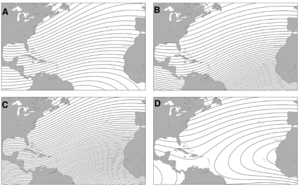
Figure 3.1 Representations of the earth’s magnetic field (Lohmann et al. 2007) The movement of the liquid outer core generates a self-exciting dynamo which produces the earth’s main-dipole magnetic. The two poles of this magnetic field correspond, approximately, to the location of the geographic north and south poles. Field lines exit the southern hemisphere and reenter the northern hemisphere and the related magnetic parameters vary systematically from the poles to the equator. This results in inherent positional information in the main-dipole field. (A) Diagrammatic representation of the Earth’s magnetic field illustrating how field lines (represented by arrows) intersect the Earth’s surface, and how inclination angle (the angle formed between the field lines and the Earth) varies with latitude. At the magnetic South Pole, field lines are directed away from the earth, perpendicular to its surface. The field lines become progressively less steep as one travels towards the magnetic equator (the thick curving line across the Earth), where the inclination angle is 0°. Then, moving from the equator towards the magnetic North Pole, field lines are directed down into the Earth and become
progressively steeper until the field lines are directed straight down into the Earth and the inclination angle is 90°. (B) Diagram illustrating four elements of geomagnetic field vectors that might, in principle, provide animals with positional information. The field present at each location on Earth can be described in terms of a total field intensity and an inclination angle. The total intensity of the field can be resolved into two vector components: the horizontal field intensity and the vertical field intensity. Sea turtles have been shown to detect total field intensity and inclination angle. Whether they (or other animals) are able of resolve the total field into vector components, however, is not known.
Exploring the geospatial organization of the magnetic map of hatchling loggerhead sea turtles
Summary
Hatchling loggerhead sea turtles (Caretta caretta) from eastern Florida undertake a
transoceanic migration in which they gradually circle the North Atlantic Ocean before returning to the North American coast. During this migration, magnetic fields that exist at widely separated
geographic areas appear to function as navigational markers, eliciting changes in the turtles’ swimming directions at crucial geographic boundaries. In principle, nearly all locations along the migratory route can be assigned to one of three geomagnetic regions: (1) the northwest Atlantic where both inclination angle and intensity of the field are greater relative to values at the home beach in Florida; (2) the northeast Atlantic where the inclination is greater but the intensity is less; (3) the southern Atlantic where both inclination and intensity are less than values at the home beach. To test the hypothesis that the geospatial organization of the loggerhead “magnetic map” consists of these three large magnetic regions, hatchlings were exposed to magnetic fields that do not exist in nature but which match the magnetic criteria of the three regions that are described above. In two of the three treatments the orientation of hatchlings was difficult to reconcile with the migratory route over the oceanic region where such fields exist. These findings imply that the magnetic map of hatchling loggerheads is not solely organized around an algorithm of enhanced or diminished intensity and inclination; at a minimum, the magnitude of field change is likely incorporated into the geospatial organization of their magnetic map.
Introduction
inclination angle (the angle at which field lines intersect the earth’s surface) steepens and the total field intensity (the strength of the field) strengthens poleward. In its simplest form, a magnetic map might provide geospatial information based entirely on whether detected magnetic field elements were increased or decreased relative to a goal field. For example, a migrating animal that encounters a steeper inclination angle and stronger intensity than the field at its geographic goal could know that it was poleward of its goal and must therefore orient equatorward. Likewise, if it encountered a less steep inclination angle and a weaker intensity than the field marking its goal, the animal could know it was equatorward of its goal and should orient poleward. In such a case, the geospatial organization of the animal’s magnetic map is to place all locations into one of two regions relative to its goal magnetic field: a poleward region and an equatorward region. Alternatively, an animal could learn or inherit a magnetic map that allows for a more precise assessment of its geographic location along its migratory route by taking into account the magnitude as well as direction of field change.
Few experiments have been designed to characterize the geospatial organization of magnetic maps (Lohmann et al. 2007). Thus it is unknown whether most animals use magnetic information in a simple, “directional” way of determining position or whether magnetic maps are more spatially complex (e.g., incorporate the magnitude of field parameters). Here, this first possibility is examined for the hatchling loggerhead sea turtles (Caretta caretta), a species with a well-established magnetic map sense.
Loggerhead hatchlings from the east coast of Florida, U.S.A. migrate offshore and are transported by the Gulf Stream northward and then eastward across the North Atlantic Ocean (Carr 1987; Bolten 2003). Loggerheads remain in the circular current system of the North Atlantic
Subtropical Gyre for 5 to 10 years before returning to their natal coast (Bjorndal et al. 2000a; Bowen & Karl 2007).
In principle, the loggerhead’s pelagic migratory route can be organized into three