NEIGHBORHOOD POLLUTION AND SUBJECTIVE HEALTH
Niobra Monique Samuel-Peterson Keah
“A thesis submitted to the faculty of the University of North Carolina at Chapel Hill in partial fulfillment of the requirements for the degree of Master of Arts in the Department of Sociology.”
Chapel Hill 2012
Approved by: Kathleen Mullan-Harris Kyle D. Crowder
ii
ABSTRACT
NIOBRA MONIQUE SAMUEL-PETERSON KEAH: Neighborhood Pollution and Subjective Health
(Under the direction of Kathleen Mullan-Harris, Kyle D. Crowder, and Neal Caren)
In response to a call for more research documenting the association between pollution and subjective health, I use data collected by The Panel Study of Income
Dynamics (PSID) between 1990 and 2007 to explore the association between neighborhood pollution and subjective health. Using regression analysis, I find that both neighborhood and individual level characteristics contribute to an association between neighborhood pollution and subjective health. Statistically, I also explore gender as a possible modifier in the proposed association and find minimal statistical support. Possible explanations for this finding are discussed in the conclusions. This research gives insight into how pollution may be associated with an individual’s well-being. An addition, conclusions expand the
implications of my findings on environmental justice campaigns and public health concerns.
DEDICATION
To God’s remarkable plan and marvelous purpose for my life;
&
iv
TABLE OF CONTENTS
LIST OF TABLES...v
Chapter I. STUDY AIMS...1
II. THEORY...4
III. LITERATURE REVIEW...11
IV. CONTRIBUTIONS...15
V. DATA & STUDY DESIGN...17
The PSID...17
The Sample...19
Neighborhood...20
Self-Rated Health (The Dependent Variable)...21
Pollution (The Focal Independent Variable)...22
Additional Control Variables………...24
VI. ANALYTIC STRATEGY…...26
VII. RESULTS...28
VIII. CONCLUSIONS...35
TABLES...39
LIST OF TABLES Table
1. Table 1. PSID Respondents by Household Status
and Gender, N=9,591...39 2. Table 1a. Percentage of PSID Respondents by
Household Status and Gender, N=9,591...39 3. Table 2. Descriptive Statistics for Variables in
Models of Subjective Health – PSID, 1990-2007………...40
4. Table 3. Average Health and Frequencies of
Health Status of PSID Sample by Sociodemographic
Characteristics (N=9,591)...41 5. Table 3a. Average Health along Sociodemographic
Characteristics, Household Status, and Gender (N=9,591)...42 6. Table 4. Ordered Logit Results for
Health Status, PSID 1990-2007...43
7. Table 4a. Ordered Logit Results for
Health Status, PSID Household Heads (N=8,223) 1990-2007………...44 8. Table 5. Linear Regression Results for Health
Status, PSID 1990-2007, N=9,591……….………45 9. Table 6. Correlation Matrix for Neighborhood
Chapter One
STUDY AIMS
The following thesis responds to the need for more studies that document associations between environmental pollution and subjective health outcomes (Brulle and Pellow 2006). Within this particular study I seek to answer the following two questions:
• Is there statistical evidence for an association between subjective health and pollution in the tract of residence?
• Does gender moderate in the proposed relationship between subjective health and pollution the tract of residence?
Using data collected by The Panel Study of Income Dynamics (PSID) between 1990 and 2007 I explore the proposed association between neighborhood pollution and subjective health. In addition, I investigate the role of gender as a possible modifier within this projected relationship. The PSID is a longitudinal survey with rich information surrounding the income, family dynamics, socioeconomic background, and health of approximately 8,289 household heads (as of 2007).
issues affecting public health to gain better insight into the patterns, and disparities in health outcomes that exist across demographic characteristics such as race/ethnicity and socioeconomic status and neighborhood context. In addition, this research will move beyond past research which has examined pollution at the country, state, and city levels (Slama et al 2007; Lederman et al 2008; Wong et al 2008) by testing the influence of pollution exposure in a given tract of residence, thus acknowledging that pollution can greatly vary across small geographic areas (Boardman et al 2008; Stuart, Mudhasakul, and Sriwatanapongse 2009). Recent literature has also highlighted disparities in exposure to pollution (Boardman et al 2008; Stuart, Mudhasakul, and Sriwatanapongse 2009; Crowder and Downey 2010). These studies find instances of environmental injustice by age, race and class. This project will aid in informing environmental justice campaigns in identifying the implications of exposure to neighborhood pollution.
3 3
Chapter Two
THEORY
Past research has explored psychological health outcomes such as mental distress (Boardman 2008); however, this study focuses on subjective health. Subjective health is the chosen health outcome variable primarily because it has not yet been studied in conjunction with neighborhood-level pollution. This individual-level health outcome allows for the control of spuriousness and individual variation in the effects of pollution on health. Subjective health is also chosen because of the unique pathways in which it links pollution and general health.
5 5
The presence of neighborhood pollution may also spark one's perception of a harmful environment and therefore lead individuals to feel as though their health is affected adversely by their surroundings (Dalton 2003; Lederman et al 2008). Moreover, these perceptions of a harmful environment may spread and develop amongst a community via social networks. As individuals in a community begin to socialize with each other about issues affecting their neighborhoods, more residents become aware of possible environmental hazards as well as the effects of those hazards (if any) on others within in the community. This knowledge could lead individuals to judge their own health more harshly regardless of whether a particular illness has been diagnosed or not. This conclusion might strengthen the likelihood of poor health outcome reports even in the absence of overt physiological problems, ultimately highlighting the argument for a psychological mechanism connecting pollution to health.
association between neighborhood socioeconomic disadvantage and individual health arguing that individual factors matter (Browning and Cagney 2003; Giatti et al 2010). My study recognizes the importance of Ross and Mirowski (2008). The researchers find that neighborhood does matter, though neighborhood has a smaller impact on health than individual sociodemographic factors (Ross and Mirowski 2008). Ross and Mirowski also conclude that “40 percent of the association between neighborhood socioeconomic status and individual health is contextual and about 60 percent is compositional” (p168, 2008). Pollution too has notable associations with neighborhood context. Researchers have found that pollution emitting facilities are more likely to be located in poor, non-white neighborhoods where companies have gained inexpensive land and face the least resistance from residents for toxic emissions (Wing et al 2000; Lipfert 2004; Brulle and Pellow 2006; Strife and Downey 2009). As a result, race and class disparities in exposure to pollution exist (Boardman et al 2008; Stuart, Mudhasakul, and Sriwatanapongse 2009; Crowder and Downey 2010). Further, researchers have concluded that this disproportionate exposure to pollution is associated with higher rates of poor health (Wing et al 2000; Brulle and Pellow 2006).
7 7
these studies find that women are better neighbors than men. Importantly, they arrive at this conclusion not because of popular notions that women spend more time in the neighborhood and work less than men (a notion that is decreasingly accurate), but instead because women in the United States are socialized to take on more social responsibility in their neighborhoods than men (Campbell and Lee 1990; 1992). While they find that both men and women exchange neighborhood goods and resources equally, when it comes to other recalled social interaction, women can name more of their neighbors, have talked with or visited with more neighbors, have a longer mean length of relationship with their neighbors and more often engage in brief “hello” interactions, as well as have longer conversations about neighborhood problems than men (Campbell and Lee 1990). As a result, Campbell and Lee (1992) provide support to the claim that women tend to have larger neighborhood networks than their counterparts and are “better neighbors” than men.
transmitted through neighborhood social networks which they are less connected to; as a result, men are less aware of the existence and probable danger of environmental harm in their neighborhood. Women, on the other hand, have stronger neighborhood ties and more neighborhood interaction which, in turn, increases the flow of information passed along social networks therefore expanding awareness of the presence and potential hazards of local pollution so that higher levels of pollution will more strongly affect women than men.
Differences in men’s and women’s social interactions in the home environment are important to the argument that perception of subjective health is gendered because perception of health may be shaped by more than just the individual. It is plausible that female labor force participation may alter the social networks of women. Despite labor force participation, women may still be more likely to maintain closer relationships with their neighbors. The literature surrounding women and the “second shift” supports this argument. Studies have shown that regardless of employment status, women still do more work taking care of the home and children (Bianchi et al 2000; Hoschild 2003; Milkie et al 2009). These at-home activities are more likely to put women in closer contact with neighbors. Due to the lack of data on neighboring within the PSID I am unable to test the empirical question of whether neighboring differences by gender arise as a result of neighborhood conditions; I do, however test the implication of these arguments on subjective health.
9 9
that women are more aware than men of their surroundings (Stern et al 1993; Schultz and Lempert 2004; Bevc, Marshall, and Picou 2007). Women talk about the advantages and disadvantages of living in a neighborhood, have opinions about neighborhood conditions and pay attention to the association between the environment and valued things (self, others, and the biosphere) regardless of whether they hold similar core values regarding environmental issues (Stern et al 1993; Schultz and Lempert 2004; Bevc, Marshall, and Picou 2007). Further, previous research finds that women tend to express more concern with technology and local1 environmental hazards than men (Mohai 1992; Davidson and Freudenburg 1996).
The implication of these findings is that even with access to the same information women may perceive greater danger from pollution, thus increasing the influence of local pollution on self-perception of health.
Based on theoretical arguments regarding the mechanisms by which pollution may affect health and variation in the influence of neighborhood and social interaction by gender, this study assesses whether an association between pollution and health exists as well as characterizes the conditioning role of gender within this association. I first examine whether subjective health tends to be lower for those in more polluted areas. After controlling for other individual factors such as, age and marital status, I expect for the association between pollution and poor subjective health to persist. Therefore, I hypothesize that subjective health is negatively influenced by increased concentrations of local pollution even after controlling for important individual and neighborhood factors. Second, I hypothesize that women’s subjective health is more strongly affected by pollution than men’s subjective health due to
1 The terms local and neighborhood will be used interchangeably throughout this thesis.
Chapter Three
LITERATURE REVIEW
pollution and health outcomes and strengthen physiological arguments for the influence of pollution on subjective health.
While prior research is consistent with theoretical arguments connecting pollution to health, it falls short of testing the influence of local/neighborhood pollution exposure on an individual-level overall indicator of health. Past research controls for various characteristics of the population that may influence both pollution and health. This body of research, however, does not utilize neighborhood-level pollution measures nor does it explore subjective health as the main dependent variable. Further, past research does not examine gender disparities in the influence pollution on subjective health.
Prior research also misses the fact that pollution varies across small areas such as neighborhoods within cities, counties, states, and countries. Studies within the more general body of pollution and health literature focus on geographically limited case-studies which pin point population-level health in one or two large, highly polluted areas such as mortality in Hong Kong (Wong et al 2008), birth outcomes in post 9/11 New York City (Lederman et al 2008), and birth weight in Munich, Germany (Slama et al 2007). These studies examine pollution at the region, state, or county level which assumes that all residents are exposed to the same averaged levels of pollution. In truth, pollution is not stagnant or evenly distributed across space; there is dramatic variation over smaller geographical units such as neighborhoods (Boardman et al 2008; Stuart Mudhasakul, and Sriwatanapongse 2009).
13 13
economic development and economic inequality at the country and county levels. For example, Sun and colleagues (2008) find that air pollution significantly affects subjective health when controlling for sociodemographic and community economic development variables. Also, in their study of pollution and health in urban areas in the continental United States, Charafeddine and Boden (2008) find that respondents in states with lower income inequality are more likely to report poor/fair health in relation to increased levels of pollution. While these studies establish that there is a relationship between pollution and subjective health and the importance of neighborhood characteristics in determining individual health, they focus specifically on the elderly (Sun et al 2008) and urban residents (Charafeddine and Boden 2008). After finding that neighborhood characteristics influence subjective health, and asserting that neighborhood context matters, past research fails to study pollution at the neighborhood level.
problems. These studies make evident the psychological argument for the influence of pollution on health.
The few studies that examine gender disparities in the relationship between pollution and health suggest that men and women may be affected by pollution differently; however, they have yet to address both neighborhood-level pollution and individual-level health on a national scale. In their 2005 Californian study, Chen et al find a statistically significant relationship between county-level pollution and risk of coronary heart disease mortality in females and not males. Chen et al (2005) focuses on a sample of mortality counts in the California area and uses county-level pollution data. Boardman and colleagues (2008) find that the negative relationship between increased industrial activity and poor mental health is more pronounced amongst women than men. Boardman et al (2008) observes solely mental health and uses neighborhood-level industrial activity data for the city of Detroit, Michigan.
Chapter Four
CONTRIBUTIONS
This research adds the present body of research by utilizing a large national sample of United States residents from a range of socioeconomic statuses, ages, races, and geographic residences to explore the possible relationship between neighborhood pollution and subjective health. Measurement issues are addressed by analyzing pollution across the nation at the neighborhood-level where a neighborhood is defined as a U.S. Census tract. The use of nationally representative data within this project allows for a sample distributed across a wide range of places. Neighborhood level pollution analysis brings forth dissimilarity in pollution exposure across smaller geographical units. This project observes the subjective health of PSID household heads, a health outcome that adds to both physiological and psychological arguments connecting pollution to health. Lastly, this study observes whether gender is a modifier in the proposed association between pollution and subjective health.
partially perceptive nature of subjective health, I am able to observe possible influences of aggregate measures of pollution as opposed to exploring specific chemical toxins (as would be done if the focus of the research were primarily on physiological pathways).
Aside from bringing forth a case in which the association between pollution and subjective health is tested, this study draws upon data that allows for a smaller and more precise census tract unit of analysis by which pollution is examined. Instead of proposing a new psychological pathway by which pollution might influence subjective health, this project provides a stronger base for existing arguments which link pollution to subjective health. While the physiological argument presented affirms that chemical factors contribute to the correlation between pollution and poor individual health maladies, the psychological argument presented in this thesis states that perception of environmental surroundings, neighboring, and concern with environmental hazards drive the association between pollution and subjective health.
Chapter Five
DATA & STUDY DESIGN
The research questions presented in this study were addressed using data from the Panel Study of Income Dynamics due to its survey design and upkeep over the years; inclusion of important control variables which impact health; ability to be linked to extensive environmental data; and inquiry into respondents’ health and well-being.
The PSID
The PSID, which began in 1968, is a large computer assisted interview survey of U.S. residents and their families. Data regarding respondents’ finances, social behavior, family dynamics, have been collected annually until 1997 and biennially after 1997. In 37 years the PSID has maintained a response rate of 96%-98% from wave to wave and grown to nearly 9,000 household heads (psidonline.umich.edu). Such low attrition rates are beneficial to the proposed study because, with the sample weights provided by the PSID, findings using these data both reduce concerns about generalizability and enhance my sample’s comparability to the PSID population as a whole. Fitzgerald et al, (1998) found that even though a large portion of the original PSID sample dropped out of the study, the representativeness of the study through 1989 was not compromised. Further, since 1989, there is no significant evidence that the PSID’s cross sectional representativeness has been compromised (Fitzgerald et al 1998).
special samples of immigrant populations in order to remedy this issue. While caution should be used in generalizing about non-black and non-white populations, they will still be included in this project’s sample population.
The PSID is well suited for the proposed study for a few key reasons. First, the PSID allows for longitudinal analysis using the individual as the unit of analysis. With this structure I will be able to utilize fixed effect modeling which will help me assess the potential role of neighborhood selection in supplemental sensitivity tests. Neighborhood selectivity refers to the individual characteristics associated with why one chooses to live in his/her
neighborhood. The relationship between socioeconomic status and pollution exposure may complicate our ability to examine associations between subjective health and pollution because low socioeconomic status may reduce an individual’s ability to select higher quality neighborhoods and lead him/her to live in more polluted areas. The primary statistical issue here is whether or not neighborhood selection will impact the parameter estimates of the association between pollution and health due to the inability to control for all individual factors (both observed and more importantly, unobserved) that affect both the likelihood of living in a polluted neighborhood and of reporting poor SRH. Individual fixed-effect modeling helps to minimize this bias by illuminating within person changes over multiple years of data collection.
19 19
research plan, a Sensitive Data Protection Plan and a signed “Contract for Use of Sensitive Data” in order to protect the anonymity of the respondents, Geocode Match Files can be linked to the tract of resident for the PSID household. PSID Household- and individual-level data are then attached to neighborhood level data. Collectively, these data will contain PSID family and individual-level responses and neighborhood characteristics including information on environmental toxins.
The Sample
My study sample will include respondents classified as household heads and wives in individual-level and family-level waves of data collected between 1990 until 20072. These years were chosen because they are years for which there are reliable pollution data and PSID data (Crowder and Downey 2010). Focus on data collected within these 17 years will provide a first look at the link between neighborhood pollution and individual health as well as the opportunity to utilize the longitudinal nature of the data. Respondents include household heads who responded for themselves and household heads’ spouses for which the household heads also responded.3 The household head is defined by the PSID as an individual who is at least 16, and holds the most financial responsibility in the household. The household heads and spouses sample is comprised of male and females ages 19-99 of various races/ethnicities. According to the PSID, a household head’s “wife” or spouse includes partners in marital unions as well as live in partners of the household head for more than one year.
2 The sample will include the following years for which PSID health data is provided: 1990, 1991, 1992, 1993, 1994, 1995, 1996, 1997, 1999, 2001, 2003, 2005, 2007 (PSID 2009).
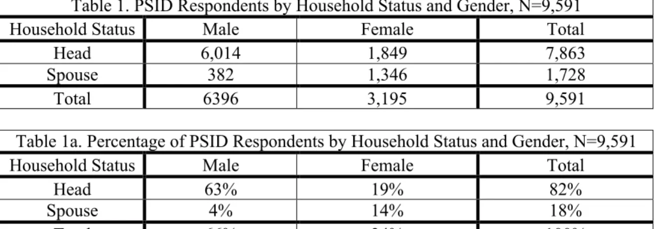
This study’s sample includes data collected over 17 years for 9,591 respondents. Table 1 shows the distribution of respondents by gender and household status. This population is made up 6, 396 males (6,014 that are heads of household) and 3, 195 females (1,849 that are heads of household). In total, the year-based sample includes 29,152 yearly (or repeated) observations over 13 data collection years. Not all respondents, however, have multiple years of data. In fact, the maximum number of years for which a respondent has multiple observations is 5 for females and 10 for males. Fifty percent of the females in the sample have between 3 and 5 years of data; whereas, 5% of males have between 5 and 10 years of data.
Neighborhood
The pollution data proposed within this study follows techniques used by Boardman et al (2008) and Crowder and Downey (2010). Because pollution is estimated at the Census tract-level, it makes sense for a neighborhood unit to be defined as a US Census tract. Census tracts are geographical areas within counties which contain between 1,500 and 8,000 persons. Census tracts typically coincide with population characteristics unique to counties and sometimes share administrative boundaries such as metropolitan areas. The spatial size of the geographic area is dependent upon an area’s population density; as the population density increases, the geographic area decreases (http://www.census.gov/geo/www/cen_tract.html).
21 21
and living circumstances into account (Census Bureau 2010). Second, the smallest level that individual-level PSID data in conjunction with Geocoded Match Files can be analyzed is the tract-level. Other pollution studies have also productively utilized this geographic level of analysis (Boardman et al 2008; Crowder and Downey 2010).
Due to the fact that this research is concerned with respondents’ perception of their neighborhood surroundings and because theoretical arguments point to social context as a key part of the mechanism by which perception is formed, whether or not tracts can socially be considered neighborhoods is an issue that cannot be ignored. It is possible that the social contexts in which individuals live make up the boundaries of a neighborhood. Census tracts are designed with population density and geographical limits in mind; however, it is still relevant to note that even though these are physical boundaries, they are also residential environments to which respondents are exposed. Census tracts are widely accepted by researchers as an acceptable measurement tool when examining geographical neighborhood boundaries today (e.g. Boardman et al 2008; Crowder and Downey 2010) and therefore will be used in this study.
Self-Rated Health (The Dependent Variable)
been collected every PSID interview year since 1987. This study will utilize responses from data collected between the years 1990 and 2007. The question specifically asks “..including any serious limitations you might have. Would you (HEAD) say your health in general is excellent, very good, good, fair, or poor?”
Pollution (The Focal Independent Variable)
23 23
combined with proximity to facility and facility size can help researchers estimate the status of pollution on individuals based on correlations between visual evidence of pollution, facility size and total emissions in relation to individuals within a tract of residence. The idea here is that while individuals may not know and discuss concrete levels of specific hazardous toxins, they do know and discuss visual evidence such as the size and proximity of industrial sites emitting pollution.
Pollution is measured using strategies employed by Boardman et al (2008), Downey (2006), and Crowder and Downey (2010). First, TRI facilities are located on a Census tract map of the U.S. and a 400 square foot rectangular grid is then placed over the map. Second, the distance from each TRI facility to the center of each grid cell is calculated. Third, weights are calculated using a distance decay function in which values decline from one to zero as distance between the facility and the grid cell increases. Weights are set to zero beyond 1.5 miles because facilities that are at 1.5 miles or more away from the center of a given tract are presumed not to influence health outcomes in that tract. Fourth, the grid weight is multiplied by the pounds of air pollution estimated to influence that grid cell. Finally, the grid cell values within a given tract are averaged together to provide a measure of proximate industrial pollution for all U.S. census tracts.
possible association between perception of neighborhood pollution and subjective health. Thus, by measuring concentrations of pollution and simultaneously proximity to pollution emitting facilities, I am likely to capture both the physiological processes via exposure and the psychological processes via proxy for perception at work.
Additional Control Variables
The comprehensive nature of the PSID allows for further isolation of the effects of environmental pollution on health. I will explore the role of correlates of subjective health mentioned and used in past literature including: gender and race (Cummings and Jackson 2008), education (Ross and Huber 1985; Ross and Wu 1996; Mirowsky and Ross 1998; Reynolds and Ross 1998; Goesling 2007), marital and employment status (Ross and Mirowsky 1995; Ferrie et al 1998; Heard et al 2008), as well as income (which has a non-linear association with health) and age (Adler et al 1994; Ross and Wu 1996; Park 2005; Subramanian and Kawachi 2006).
Racial categories within the PSID include: White; Black, African-American, or Negro; Asian; and Native Hawaiian or Pacific Islander. While race will be controlled in this study, specific racial variations will be explored in future research. Age and education will be left as a continuous variable while income will be standardized to 2007-equivalent values in order to account for inflation.
25 25
live close to where they work (possibly more heavily polluted neighborhoods) and would therefore have a higher exposure to more pollution on the job. Marital status includes: married; never married; widowed; divorced/annulled; and separated.
This study uses select neighborhood variables with strong ties to the dependent variable and main independent variable. Neighborhood context is taken into account by examining respondents’ neighborhood racial profile (percent minority), and income (average family income), all in the tract of residence.4
Chapter Six
ANALYTIC STRATEGY
To study the associations between local pollution and subjective health over PSID study years between 1990 and 2007, I use ordered logit regression models with robust standard errors for clustering at the individual level. Ordered logit models allow for regression analysis that is able to utilize the full five-response health variable. These regression models measure the variance across individuals but may produce biased results because they do not take into account selection processes and unobserved individual-level characteristics influencing both health and exposure to pollution. Despite these limitations, ordered logit regression models are preferred because they allow for full variance in the subjective health variable to be observed.5 This study also utilizes multiple levels of analysis presented in the independent variables. Multilevel variables are useful to this study because they allow for the disaggregation of error structures over observational and individual levels of collection. Concerns regarding correlated error terms due to with-in person repeated observations are adjusted for by clustering observations on respondents’ unique identifying variables.
27 27
Chapter Seven
RESULTS
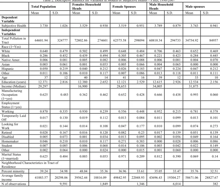
The study population incorporates 9,591 male and female PSID respondents and their spouses (see Table 1 and Table 1a). Sixty-three percent of household heads in the sample are male and 19% are female. There are 1,728 spouses in the sample; around 42% of females in the sample are spouses (see Table 1). Table 2 provides descriptive statistics for all of the variables used in this study. The age range of respondents in the sample spans from 16-98; the mean age of the population is 37. Average education attained in years is the equivalent of a high school education. The average respondent is married and working. Both characteristics are associated with better overall wellbeing. Sixty-two percent of the respondents report working in a manufacturing occupation that, in nature, may increase a respondents’ exposure to pollution.
29 29
and women (household heads and spouses) in the sample are comparable, around 12 years. The median income for male heads of household ($34,005) is more than double the median income for female household heads ($16,900); however the median income for male and female spouses shows less of a gap ($31,875 and $28,653, respectively). Married heads of household report a median income of $38,294 while the median income for unmarried heads of heads of household is only $17,850.
Finally, in Table 2 we see relative differences in neighborhood characteristics. On average, females household heads in the sample live in neighborhoods with higher percentages of minorities (48%) compared to female spouses who tend to live in neighborhoods with lower percentages of minorities (36%). In addition, female household heads in the sample tend to live in neighborhoods with lower average family incomes than female spouses ($39,562 and $49,842, respectively), while male household heads in the sample live in neighborhoods with lower average family incomes than male spouses ($43,696 and $58,671, respectively). Differences in employment status of male and female spouses may contribute to differences in neighborhood average family incomes by raising the total household income and making higher income neighborhoods accessible. Table 2 shows that while 78% of male spouses are currently working, only 55% of female spouses are working. These results highlight the sample characteristics of respondents and their surrounding environments for which health is being predicted, however, I note that the female head sample is over-represented by single mothers in the sample, thus somewhat limiting the neighborhood variation for them.
31 31
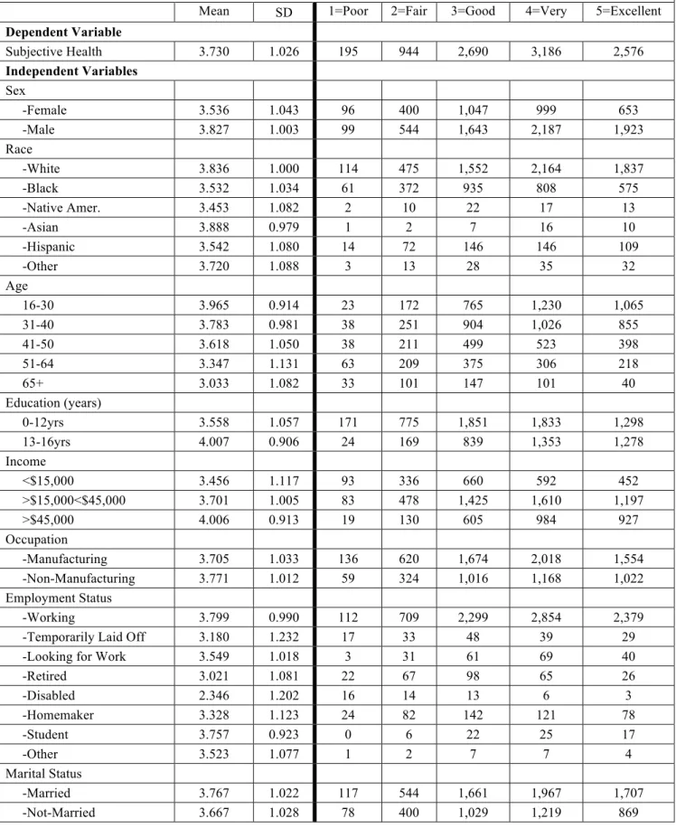
influence subjective health (Ross and Huber 1985; Adler et al 1994; Ross and Mirowsky 1995; Ross and Wu 1996; Ferrie et al 1998; Mirowsky and Ross 1998; Reynolds and Ross 1998; Park 2005; Subramanian and Kawachi 2006; Goesling 2007; Cummings and Jackson 2008; Heard et al 2008).
Table 3a presents averages in subjective health by household status. Results show that for all racial groups, female heads of household have lower averages of subjective health than male heads of household. The same trend is present for all sociodemographic characteristics except for two employment status variables: temporarily laid off and homemaker, where female household heads have a higher average subjective health than male household heads.
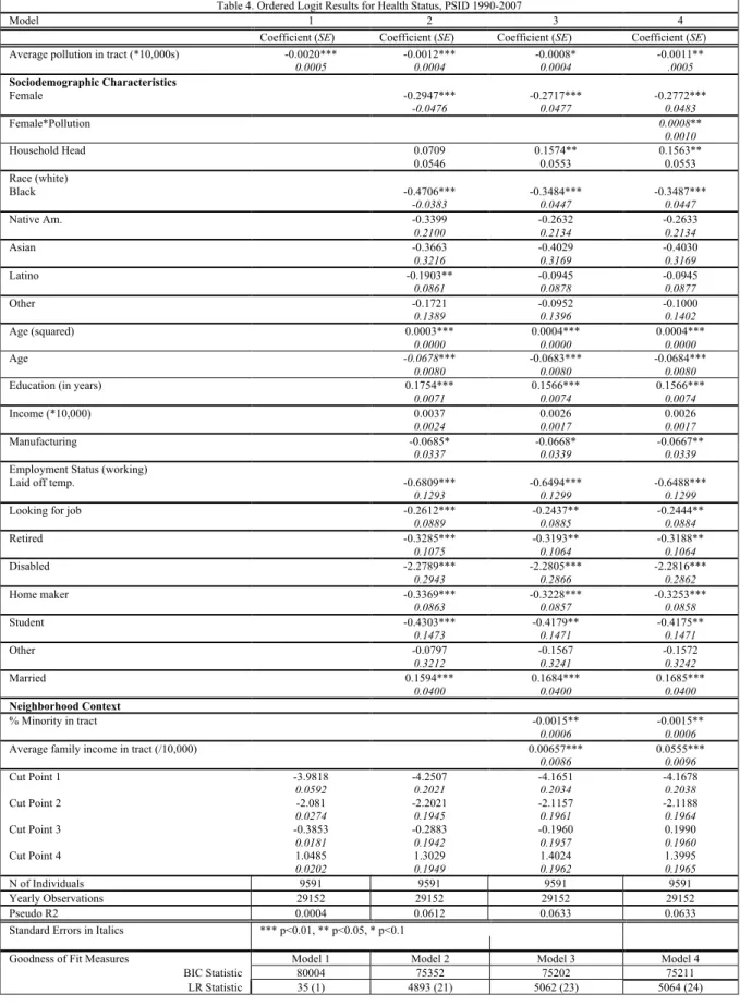
In Table 4 I move forward to describe the association between pollution and subjective health using ordered logit models. Model 1 predicts subjective health using pollution. This model is estimated using 5 parameters, 1 independent variable and 4 cut points. The cut points numerically represents numerical thresholds between categorical outcomes. The pollution coefficient in this model confirms that excellent health is negatively correlated with increasing pollution. The log odds of reporting an increase in health status (i.e., better health) reduce by 0.1 percent with every 10,000 unit increase in pollution.6 At the most basic level, this model supports the hypothesis that subjective health is negatively influenced by increased concentrations of local pollution.
Model 2 includes socio-demographic controls that are theoretically linked to both health status and exposure to pollution. With these additional controls, Model 2 shows that
pollution is still associated with health; however, some of this association can be explained by sociodemographic characteristics. Most specifically, Model 2 shows that nearly all of the added independent variables are important correlates of health. For example, in concert with theory, age has a negative association with health, whereas income and education have a positive association with health. Marital status also has a positive association with health. Black and Hispanic respondents are statistically significant correlates of health. Also in Model 2 I find that every $10,000 increase in individual level income is associated with a 0.4 percent (i.e., (e.0037-1) X 100) increase in log odds of reporting good health.
While small, the effect size of pollution can more easily be seen in comparison with average family income in the census tract. For example, in Model 3, one standard deviation increase in pollution exposure is associated with a 0.000025 decrease in the ordinal scale of health while a one standard deviation increase in average family income in tract is associated with a .003 increase in the ordinal health scale. The association of neighborhood pollution with health is therefore quite small relative to the association of average neighborhood income with health, even with individual and other neighborhood characteristics taken into account.
33 33
BIC goodness of fit tests show that Models 2 and 3 are better able to predict health. Variance in BIC between Models 2 and 3 are very small. Psuedo R2 also tells us that the most variation in health is explained in model 3 (0.0618). These statistical differences may be representative of the magnitude of neighborhood characteristics on self-rated health.
Results surrounding the role of gender in the association between pollution and subjective health are also explored in Table 4. In Model 4, the interaction between pollution and gender is added. In Model 4 the product term is statistically insignificant; however, the coefficient for the product term is in the negative direction. Supplemental statistical tests show that the addition of the product term does not significantly improve Model 3 (prob>chi2 = 0.4768)7. While females more often report having poorer health than men, there is not strong evidence that gender moderates the association between pollution and health.
In Table 4a I report results that estimate ordered logit models using solely PSID household heads in order to bring forth differences that may exist between male and female household heads and to test the sensitivity of spousal reporting of subjective health. Results show similarities in the direction of the association between pollution and subjective health in the sample of household heads and in the full sample of household heads and spouses.
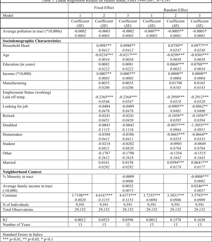
Table 5 presents results using fixed effects linear regression models using the entire sample population to check the sensitivity of the ordered logit models (1-3) used within this study (see Table 5). This method of comparison treats self-rated health as a linear dependent variable. It is valid to think of self-rated health as linear because unlike other clearly ordered
measures (e.g. physical activity: never, monthly, weekly, daily), self-rated health is nearly linear in its category construction. Using linear models to estimate models with the 5-category self-rated health indicator is not unusual (see Burgard, Brand and House 2007). By adding the fixed effect and random effect linear comparison, I am able to compare results that take account of unobserved variation within individuals across time (i.e., fixed effects) and their potential influence on self-rated health in the random effects models.
Chapter Eight
CONCLUSIONS
This study provides empirical evidence for an association between neighborhood pollution and subjective health. While some of this association can be explained by sociodemographic and neighborhood factors, as pollution exposure increases, the likelihood of reporting poor health increases This finding is consistent with documented associations between pollution and other psychological and physiological health outcomes (Lima 2004; Chen 2005; Bevc, Marshall, and Picou 2007; Boardman et al 2008; Charafeddine and Boden 2008; Sun et al 2008). In addition, this study adds further support to prior research that has found sociodemographic and neighborhood characteristics to be important factors contributing to health status (Ross and Huber 1985; Adler et al 1994; Ross and Mirowsky 1995; Ross and Wu 1996; Ferrie et al 1998; Mirowsky and Ross 1998; Reynolds and Ross 1998; Park 2005; Subramanian and Kawachi 2006; Goesling 2007; Cummings and Jackson 2008; Heard et al 2008). Though increases in average units of pollution in a tract are associated with very small declines in subjective health, these declines are significant, meaning it is highly unlikely that the decline shown in the results is by chance. This suggests that exposure to neighborhood pollution is correlated with one’s well-being psychologically.
association between pollution and subjective health. First, the majority of the women in the sample were working or looking for a job. Results show that employment status does attenuate the association between pollution and subjective health (along with other factors). Perhaps the subjective health of working women is influenced by pollution in a similar manner to how men’s subjective health is influenced by pollution. The gender effect is stronger in Table 4A (for female household heads) than in Table 4 (all women, household heads and spouses), but it is difficult to discern whether it is the employment status of female household heads or something else that matters.
Second, research has uncovered the importance of weak ties in the social world. Scholars have found that weak ties are important to social networks and the dissemination of information (Granovetter 1973; Thoits 2011). This suggests that weaker social ties within a neighborhood across men and women may more widely spread the word of environmental hazards than strong ties. Therefore, while women may have deeper social networks, men may still receive the same information through their weak social ties.
37 37
In spite of non-statistically significant findings surrounding the role of gender in the association between pollution and health and limitations in the data, this research brings to light important thoughts on how environmental injustice may affect social groups differently. Pollution emitting facilities position themselves in areas with lower property values and where they will face the least community resistance (Wing et al 2000; Lipfert 2004; Brulle and Pellow 2006; Strife and Downey 2009). The question for researchers then becomes how does one assess the presence of these facilities on the community that is being exploited? This study may be one step in the right direction by exploring pollution at the neighborhood level and its role in a health outcome that has social, psychological, and physiological ties.
The findings of this study point to race, class and age inequities in subjective health and exposure to pollution. Research on environmental racism reports that minority and poor populations (especially in rural areas) are disproportionately exposed to higher concentrations of pollution (Wing et al 2000; Lipfert 2004; Brulle and Pellow 2006; Strife and Downey 2009). Upcoming studies should further explore the role of race/ethnicity, class, and age in the association between pollution and subjective health.
39 39
TABLES
Table 1. PSID Respondents by Household Status and Gender, N=9,591
Household Status Male Female Total
Head 6,014 1,849 7,863
Spouse 382 1,346 1,728
Total 6396 3,195 9,591
Table 1a. Percentage of PSID Respondents by Household Status and Gender, N=9,591
Household Status Male Female Total
Head 63% 19% 82%
Spouse 4% 14% 18%
Table 2. Descriptive Statistics for Variables in Models of Subjective Health – PSID, 1990-20078
Total Population Females Household Heads Female Spouses Male Household Heads Male spouses
Mean S.D. Mean S.D. Mean S.D. Mean S.D. Mean S.D.
Dependent
Variable
Subjective Health 3.730 1.026 3.529 0.930 3.519 0.951 3.789 0.879 3.743 0.941
Independent
Variables
Total Pollution in
Tract 64601.94 324777 72802.86 274601 62575.58 298094 60810.34 294733 34754.92 84957
Race (1=Yes)
White 0.640 0.479 0.502 0.499 0.648 0.484 0.706 0.463 0.652 0.469
Black 0.286 0.452 0.439 0.494 0.305 0.467 0.221 0.423 0.284 0.445
Native Amer. 0.006 0.081 0.005 0.082 0.006 0.088 0.006 0.081 0.004 0.070
Asian 0.003 0.061 0.001 0.053 0.005 0.066 0.004 0.065 0.000 0.000
Hispanic 0.050 0.219 0.040 0.212 0.026 0.183 0.047 0.224 0.047 0.212
Other 0.011 0.106 0.010 0.117 0.007 0.086 0.013 0.118 0.011 0.111
Age 37 12 40 14 41 16 39 12 33 10
Education (years) 12.371 2.816 12.380 2.652 12.121 2.529 12.615 2.926 12.534 2.156
Income (Median) 29,297 16,900 28,653 34,005 31,875
Manufacturing Occupation (1=yes)
0.625 0.483 0.362 0.462 0.652 0.428 0.666 0.438 0.993 0.060
Employment
Status (1=yes)
Working 0.870 0.335 0.930 0.239 0.556 0.448 0.952 0.215 0.781 0.378
Temporarily Laid
Off 0.017 0.130 0.019 0.112 0.013 0.084 0.011 0.099 0.013 0.101
Looking for
Work 0.021 0.144 0.014 0.108 0.047 0.177 0.010 0.099 0.074 0.273
Retired 0.028 0.167 0.016 0.120 0.082 0.23 0.017 0.139 0.051 0.139
Disabled 0.005 0.073 0.001 0.034 0.013 0.095 0.002 0.056 0.049 0.164
Homemaker 0.046 0.210 0.010 0.117 0.271 0.383 0.000 0.028 0.006 0.086
Student 0.007 0.085 0.006 0.068 0.014 0.106 0.003 0.042 0.022 0.149
Other 0.002 0.064 0.000 0.024 0.000 0.015 0.001 0.060 0.000 0.000
Marital Status
(1=married) 0.625 0.484 0.003 0.053 0.971 0.209 0.812 0.390 0.069 0.14
Neighborhood Characteristics in Tract of
Residence
Percent minority 39.24 34.98 48.04 35.36 36.96 33.61 35.05 33.47 35.76 32.51
Average family
income 41883.57 20298.06 39562.44 18816.09 49842.95 22048.93 43696.43 19304.27 58671.06 28827.67
N of observations 9,591 1,849 1,346 6,014 382
41 41
Table 3. Average Health and Frequencies of Health Status of PSID Sample by Sociodemographic Characteristics (N=9,591)
Mean
Health SD
1=Poor Health 2=Fair Health 3=Good Health 4=Very Good Health 5=Excellent Health Dependent Variable
Subjective Health 3.730 1.026 195 944 2,690 3,186 2,576 Independent Variables
Sex
-Female 3.536 1.043 96 400 1,047 999 653
-Male 3.827 1.003 99 544 1,643 2,187 1,923
Race
-White 3.836 1.000 114 475 1,552 2,164 1,837
-Black 3.532 1.034 61 372 935 808 575
-Native Amer. 3.453 1.082 2 10 22 17 13
-Asian 3.888 0.979 1 2 7 16 10
-Hispanic 3.542 1.080 14 72 146 146 109
-Other 3.720 1.088 3 13 28 35 32
Age
16-30 3.965 0.914 23 172 765 1,230 1,065
31-40 3.783 0.981 38 251 904 1,026 855
41-50 3.618 1.050 38 211 499 523 398
51-64 3.347 1.131 63 209 375 306 218
65+ 3.033 1.082 33 101 147 101 40
Education (years)
0-12yrs 3.558 1.057 171 775 1,851 1,833 1,298
13-16yrs 4.007 0.906 24 169 839 1,353 1,278
Income
<$15,000 3.456 1.117 93 336 660 592 452
>$15,000<$45,000 3.701 1.005 83 478 1,425 1,610 1,197
>$45,000 4.006 0.913 19 130 605 984 927
Occupation
-Manufacturing 3.705 1.033 136 620 1,674 2,018 1,554 -Non-Manufacturing 3.771 1.012 59 324 1,016 1,168 1,022
Employment Status
-Working 3.799 0.990 112 709 2,299 2,854 2,379 -Temporarily Laid Off 3.180 1.232 17 33 48 39 29 -Looking for Work 3.549 1.018 3 31 61 69 40
-Retired 3.021 1.081 22 67 98 65 26
-Disabled 2.346 1.202 16 14 13 6 3
-Homemaker 3.328 1.123 24 82 142 121 78
-Student 3.757 0.923 0 6 22 25 17
-Other 3.523 1.077 1 2 7 7 4
Marital Status
Table 3a. Average Health along Sociodemographic Characteristics, Household Status, and Gender (N=9,591)
Household Head Spouse Household Head Spouse
Female
Household Heads
SD Female
Spouses SD
Male Household
Heads
SD Male
Spouses SD
Dependent Variable
Subjective Health 3.546 1.036 3.523 1.053 3.831 1.007 3.746 0.940
Independent Variables
Race
-White 3.739 1.003 3.603 1.049 3.903 1.050 3.869 0.985
-Black 3.369 1.016 3.373 1.052 3.674 1.052 3.560 0.868
-Native Amer. 2.667 1.225 3.333 0.985 3.683 1.035 3.000 0.000
-Asian 3.667 0.577 4.286 0.756 3.808 1.059 0.000 0.000
-Hispanic 3.297 1.188 3.372 0.926 3.637 1.047 3.357 1.336
-Other 3.619 0.865 3.333 1.500 3.789 1.123 3.800 0.447
Age
16-30 3.871 0.899 3.856 0.884 4.035 0.927 3.915 0.873
31-40 3.526 0.981 3.538 0.999 3.894 0.961 3.663 0.941
41-50 3.392 1.062 3.525 1.121 3.695 1.029 3.480 1.035
51-64 3.145 1.142 3.134 1.107 3.472 1.118 3.400 0.986
65+ 3.037 1.084 2.797 1.069 3.272 1.045 2.800 1.304
Education (years)
0-12yrs 3.406 1.054 3.362 1.059 3.659 1.051 3.559 0.963
13-16yrs 3.779 0.959 3.896 0.940 4.086 0.878 4.095 0.799
Income
<$15,000 3.439 1.086 3.067 1.178 3.586 1.103 3.454 1.069
>$15,000<$45,000 3.595 0.991 3.554 0.988 3.768 1.014 3.693 0.916
>$45,000 3.864 0.915 3.842 0.945 4.036 0.909 4.015 0.843
Occupation
-Manufacturing 3.594 1.036 3.410 1.094 3.787 1.013 3.763 0.942
-Non-Manufacturing 3.516 1.035 3.764 0.918 3.918 0.990 4.00 0.000
Employment Status
-Working 3.581 1.025 3.744 0.934 3.871 0.980 3.821 0.921
-Temporarily Laid Off 3.352 1.097 3.523 0.928 3.056 1.337 3.200 0.447
-Looking for Work 3.273 0.977 3.441 0.983 3.746 1.079 3.625 0.942
-Retired 2.824 0.999 2.900 1.115 3.153 1.056 3.143 1.345
-Disabled 1.333 0.577 2.167 1.098 2.400 1.392 2.818 0.982
-Homemaker 3.229 1.140 3.349 1.125 2.200 0.447 3.667 0.577
-Student 3.438 0.964 3.695 0.876 3.857 1.014 4.200 0.632
-Other 3.000 0.000 5.000 0.000 3.473 1.073 0.000 0.000
Marital Status
-Married 3.857 0.690 3.504 1.056 3.840 1.002 3.000 0.816
43 43
Table 4. Ordered Logit Results for Health Status, PSID 1990-2007
Model 1 2 3 4
Coefficient (SE) Coefficient (SE) Coefficient (SE) Coefficient (SE)
Average pollution in tract (*10,000s) -0.0020*** -0.0012*** -0.0008* -0.0011**
0.0005 0.0004 0.0004 .0005
Sociodemographic Characteristics
Female -0.2947*** -0.2717*** -0.2772***
-0.0476 0.0477 0.0483
Female*Pollution 0.0008**
0.0010
Household Head 0.0709 0.1574** 0.1563**
0.0546 0.0553 0.0553
Race (white)
Black -0.4706*** -0.3484*** -0.3487***
-0.0383 0.0447 0.0447
Native Am. -0.3399 -0.2632 -0.2633
0.2100 0.2134 0.2134
Asian -0.3663 -0.4029 -0.4030
0.3216 0.3169 0.3169
Latino -0.1903** -0.0945 -0.0945
0.0861 0.0878 0.0877
Other -0.1721 -0.0952 -0.1000
0.1389 0.1396 0.1402
Age (squared) 0.0003*** 0.0004*** 0.0004***
0.0000 0.0000 0.0000
Age -0.0678*** -0.0683*** -0.0684***
0.0080 0.0080 0.0080
Education (in years) 0.1754*** 0.1566*** 0.1566***
0.0071 0.0074 0.0074
Income (*10,000) 0.0037 0.0026 0.0026
0.0024 0.0017 0.0017
Manufacturing -0.0685* -0.0668* -0.0667**
0.0337 0.0339 0.0339
Employment Status (working)
Laid off temp. -0.6809*** -0.6494*** -0.6488***
0.1293 0.1299 0.1299
Looking for job -0.2612*** -0.2437** -0.2444**
0.0889 0.0885 0.0884
Retired -0.3285*** -0.3193** -0.3188**
0.1075 0.1064 0.1064
Disabled -2.2789*** -2.2805*** -2.2816***
0.2943 0.2866 0.2862
Home maker -0.3369*** -0.3228*** -0.3253***
0.0863 0.0857 0.0858
Student -0.4303*** -0.4179** -0.4175**
0.1473 0.1471 0.1471
Other -0.0797 -0.1567 -0.1572
0.3212 0.3241 0.3242
Married 0.1594*** 0.1684*** 0.1685***
0.0400 0.0400 0.0400
Neighborhood Context
% Minority in tract -0.0015** -0.0015**
0.0006 0.0006
Average family income in tract (/10,000) 0.00657*** 0.0555***
0.0086 0.0096
Cut Point 1 -3.9818 -4.2507 -4.1651 -4.1678
0.0592 0.2021 0.2034 0.2038
Cut Point 2 -2.081 -2.2021 -2.1157 -2.1188
0.0274 0.1945 0.1961 0.1964
Cut Point 3 -0.3853 -0.2883 -0.1960 0.1990
0.0181 0.1942 0.1957 0.1960
Cut Point 4 1.0485 1.3029 1.4024 1.3995
0.0202 0.1949 0.1962 0.1965
N of Individuals 9591 9591 9591 9591
Yearly Observations 29152 29152 29152 29152
Pseudo R2 0.0004 0.0612 0.0633 0.0633
Standard Errors in Italics *** p<0.01, ** p<0.05, * p<0.1
Goodness of Fit Measures Model 1 Model 2 Model 3 Model 4
BIC Statistic 80004 75352 75202 75211
LR Statistic 35 (1) 4893 (21) 5062 (23) 5064 (24)
9 Wald test results show that the addition of a gender-pollution interaction term does not statistically improve
Table 4a. Ordered Logit Results for Health Status, PSID Household Heads (N=8,223) 1990-2007
Model 3 4
Coefficient (SE) Coefficient (SE)
Average pollution in tract (*10,000s) -0.0008* -0.0012**
0.0004 0.0005
Sociodemographic Characteristics
Female -0.3006*** -0.3156***
0.0592 0.0598
Female*Pollution 0.0021**
0.00109 Race (white)
Black -0.3428*** -0.3442***
0.0485 0.0485
Native Am. -0.1905 -0.1911
0.2339 0.2338
Asian -0.7089** -0.7100**
0.3139 0.3140
Latino -0.0838 -0.0853
0.0947 0.0944
Other -0.1058 -0.1203
0.1483 0.1495
Age (squared) 0.0005*** 0.0005***
0.0001 0.0001
Age -0.0785*** -0.0786***
0.0091 0.0091
Education (in years) 0.1564*** 0.1564***
0.0079 0.0079
Income (*10,000) 0.0028* 0.0028*
0.0016 0.0016
Manufacturing -0.0456 -0.0453
0.0368 0.0368
Employment Status (working)
Laid off temp. -0.7309*** -0.7284***
0.1545 0.1545
Looking for job -0.0905 -0.0906
0.1182 0.1185
Retired -0.3722** -0.3734**
0.1240 0.1240
Disabled -2.3875*** -2.3872***
0.4231 0.4231
Homemaker -0.3894 -0.3904
0.2729 0.2738
Student -0.3294 -0.3269
0.2111 0.2109
Other -0.3767 -0.3780
0.3157 0.3158
Married 0.1555** 0.1549**
0.0509 0.0509
Neighborhood Context
% Minority in tract -0.0013** -0.0013**
0.0006 0.0006
Average family income in tract (/10,000) 0.0637*** 0.0638***
0.0097 0.0097
Cut Point 1 -45963 -4.600
0.2211 0.2212
Cut Point 2 -2.4420 -2.4484
0.2111 0.2111
Cut Point 3 -0.5240 -0.5301
0.2104 0.2105
Cut Point 4 1.0649 1.0590
0.2107 0.2108
N of Individuals 8,223 8,223
Total Observations 24,467 24,467
Pseudo R2 0.0573 0.0574
Standard Errors in Italics *** p<0.01, ** p<0.05, * p<0.1
Goodness of Fit Measures Model 1 Model 2
BIC Statistic 62876 62881
45 45
Table 5. Linear Regression Results for Health Status, PSID 1990-2007, N=9,591
Fixed Effect Random Effect
Model 1 2 3 1 2 3
Coefficient (SE) Coefficient (SE) Coefficient (SE) Coefficient (SE) Coefficient (SE) Coefficient (SE)
Average pollution in tract (*10,000s) -0.0002 -0.0003 -0.0002 -0.0007** -0.0005** -0.0003*
0.0003 0.0003 0.0003 0.0002 0.0001 0.0001
Sociodemographic Characteristics
Household Head 0.0987** 0.0988** 0.0750** 0.0977***
0.0412 0.0412 0.0247 0.0248
Age -0.0224*** -0.0217*** -0.0299*** -0.0303***
0.0034 0.0036 0.0038 0.0038
Education (in years) 0.0082 0.0081 0.0868*** 0.0788***
0.0222 0.0222 0.0032 0.0034
Income (*10,000) 0.0007** 0.0007** 0.0008** 0.0008**
0.0003 0.0003 0.0004 0.0004
Manufacturing 0.0035 0.0035 0.01708 0.0165
0.0206 0.0206 0.0165 0.0143
Employment Status (working)
Laid off temp. -0.2365*** -0.2364*** -0.2950*** -0.2912***
0.0546 0.0547 0.0518 0.0520
Looking for job -0.0484 -0.0489 -0.0905** -0.0862**
0.0476 0.0476 0.0401 0.0400
Retired -0.0241 -0.0241 -0.1058** -0.1056**
0.0451 0.0450 0.0395 0.0394
Disabled -0.0043 -0.0042 -0.4937*** -1.5055***
0.1115 0.1116 0.0964 0.0951
Homemaker -0.0388 -0.0386 -0.0663*** -0.0664**
0.0411 0.0411 0.0335 0.0333
Student -0.0218 -0.0202 -0.0903 -0.0849
0.0821 0.0820 0.0704 0.0704
Other -0.1787 -0.1790 -0.1354 -0.1515
0.2612 0.2618 0.1642 0.1643
Married 0.0161 0.0158 0.0594*** 0.0641***
0.0292 0.0292 0.0178 0.0177
Neighborhood Context
% Minority in tract -0.0009 -0.0008***
0.0006 0.0002
Average family income in tract 0.0032 0.0246***
(/10,000) 0.0073 0.0037
Constant 3.7198*** 4.6167*** 4.6373*** 3.7255*** 3.5831*** 3.5793***
0.0020 0.3155 0.3153 0.0094 0.0906 0.0909
N of Individuals 9,591 9,591 9,591 9,591 9,591 9,591 Total Observations 29,152 29,152 29,152 29,152 29,152 29,152
R2 0.0012 0.0523 0.0596 0.0012 0.1578 0.1630
Number of Years 13 13 13 13 13 13
Table 6. Correlation Matrix for Neighborhood Level Variables (Tract of Residence) % Minority Avg. Family
Income % Female Heads of Household % Poverty
% Minority 1
Avg. Family Income -0.3998* 1
% Female Heads of Household 0.7045* -0.4770* 1
% Poverty 0.6416* -0.6069* 0.7258* 1
47 47
REFERENCES
Adler, M. A. (1994). Male-female power differences at work – A comparison of supervisors and policy-makers. Sociological Inquiry, 64(1), 37-55.
Andersen, Z. J., Wahlin, P., Raaschou-Nielsen, O., Scheike, T., & Loft, S. (2007). Ambient particle source apportionment and daily hospital admissions among children and elderly in Copenhagen. Journal of Exposure Science and Environmental
Epidemiology, 17(7), 625-636.
Barnett, A. G., Williams, G. M., Schwartz, J., Best, T. L., Neller, A. H., Petroeschevsky, A. L., et al. (2006). The effects of air pollution on hospitalizations for cardiovascular disease in elderly people in Australian and New Zealand cities. Environmental Health Perspectives, 114(7), 1018-1023.
Bell, M. L., Ebisu, K., & Belanger, K. (2007). Ambient air pollution and low birth weight in Connecticut and Massachusetts. Environmental Health Perspectives, 115(7), 1118-1124.
Bevc, C. A., Marshall, B. K., & Picou, J. S. (2007). Environmental Justice and toxic exposure: Toward a spatial model of physical health and psychological well-being.
Social Science Research, 36(1), 48-67.
Bianchi, Suzanne M., Melissa A. Milkie, Liana C. Sayer and John P. Robinson. 2000. "Is anyone doing the housework? Trends in the gender division of household
labor." Social Forces 79, no.1 (September): 191-228.
Boardman, J. D., Downey, L., Jackson, J. S., Merrill, J. B., Saint Onge, J. M., & Williams, D. R. (2008). Proximate industrial activity and psychological distress. Population and Envioronment, 30(1-2), 3-25.
Brulle, R. J., & Pellow, D. N. (2006). Environmental justice: Human health and environmental inequalities. Annual Review of Public Health, 27, 103-124.
Burgard, S.A., Brand, J.E. & House, J.S. (2007). Toward a Better Estimation of the Effect of job Loss on Health. Journal of Health and Social Behavior, 48(12), 369-384.
Burra, T. A., Elliott, S. J., Eyles, J. D., Kanaroglou, P. S., Wainman, B. C., & Muggah, H. (2006). Effects of residential exposure to steel mills and coking works on birth weight and preterm births among residents of Sydney, Nova Scotia. Canadian
Geographer-Geographe Canadien, 50(2), 242-255.
Campbell, K. E., & Lee, B. A. (1992). Sources of personal neighbor networks – social integration, need, or time. Social Forces, 70(4 Fitzgerald), 1077-1100.
Census Bureau. (2010). http://www.census .gov/geo/www/cen_tract.html.
Charafeddine, R., & Boden, L. I. (2008). Does income inequality modify the association between air pollution and health? Environmental Research, 106(1), 81-88. Chen, Lie Hong, Knutsen S.F., Shavlik D., Beeson W.L., Petersen F., Ghamsary M., &
David Abbey D. (2005). “The Association between Fatal Coronary Heart Disease and Ambient Particulate Air Pollution: Are Females at Greater Risk?” Environtal Health Prospectives, 113, 723-1729.
Chen, Y., Craig, L., & Krewski, D. (2008). Air quality risk assessment and management.
Journal of Toxicology and Environmental Health, Part A, 24-39.
Crowder, K., & Downey, L., (2010). Inter-neighborhood migration, race, and environmental hazards: modeling micro-level processes of environmental inequality. American Journal of Sociology.
Cummings, J. L., & Jackson, P. B. (2008). Race, gender, and SES disparities in self-assessed health, 1974-2004. Research on Aging, 30(2), 137-168.
Dalton, P. (2003). Upper airway irritation, odor perception and health risk due to airborne chemicals. Toxicology Letters, 140-141, 239-248.
Davidson, D. J., & Freudenburg, W. R. (1996). Gender and environmental risk concerns - A review and analysis of available research. Environment and Behavior, 28(3), 302-339. Diez-Roux, A. V. (2001). Investigating Neighborhood and Area Effects on Health. American
Journal of Public Health. 91(11), 1783-1789.
Delfino, R. J., Chang, J., Wu, J., Cizao, R., Tjoa, T., Nickerson, B., Cooper, D., Gillen, D. L. (2009). Repeated hospital encounters for asthma in children and exposure to traffic-related air pollution near the home. Annual Allergy Asthma Immunology, 102, 138-144.
Do, D. P. & Finch, K. F. (2008). The link between neighborhood poverty and health: context or composition? American Journal of Epidemiology. 168(6), 611-619.
Dominici, F., Sheppard, L., & Clyde, M. (2003). Health effects of air pollution: A statistical review. International Statistical Review, 71(2), 243-276.