ADVANCED BIOSTATISTICAL METHODS FOR CURVED AND CENSORED BIOMEDICAL DATA
Emil A. Cornea
A dissertation submitted to the faculty at the University of North Carolina at Chapel Hill in partial fulfillment of the requirements for the degree of Doctor of Philosophy in
the Department of Biostatistics in the Gillings School of Global Public Health.
Chapel Hill 2014
Approved by:
ABSTRACT
EMIL A. CORNEA: Advanced Biostatistical Methods for Curved and Censored Biomedical Data
(Under the direction of Joseph G. Ibrahim and Hongtu T. Zhu)
This research was dedicated to analyze two types of biomedical data: curved data lying on a manifold and censored survival data from clinical trials.
The main part of the research aims at developing a general regression framework for the analysis of a manifold-valued response in a Riemannian symmetric space (RSS) and its association with Euclidean covariates of interest, such as age. Such data arises frequently in medical imaging, computational biology, and computer vision, among many others. We developed an intrinsic regression model solely based on an intrinsic conditional moment assumption, avoiding specifying any parametric distribution on RSS. We proposed various link functions from the Euclidean space of covariates to the RSS of responses. We constructed parameter estimates and test statistics, and deter-mined their asymptotic distributions and geometric invariant properties. Simulation studies were used to evaluate the finite sample properties of our method. We applied our model to investigate the association between covariates, including gender, age, and diagnosis, and the shape of the Corpus Callosum contours from the Alzheimer’s Disease Neuroimaging Initiative dataset, in both cross-sectional and longitudinal cases.
To My Daughters, Christiana and Andreea, and
ACKNOWLEDGMENTS
I would like to take this opportunity to express my sincere appreciation to all the people who encouraged and supported me throughout the years.
In particular, I would like to extend my deepest gratitude to Dr. Joseph Ibrahim and Dr. Hongtu Zhu, my advisors, for their inspired guidance, encouragement throughout the ups and downs of this work, and generous help far beyond conventional limits, both academic and non-academic, that made the completion of this dissertation possible. The experience I have gained working with them is invaluable.
I would also like to acknowledge the deepest influence on my mathematical back-ground and the great appreciation of my former advisors, the late Professors Björn Jawerth and Martin Jurchescu.
I thank my committee members Dr. Amy Herring and Dr. Donglin Zeng for nu-merous, very enriched and helpful discussions throughout the past years. Thanks are also extended to Dr. Martin Styner, who served as a member of my committee.
TABLE OF CONTENTS
LIST OF TABLES . . . x
LIST OF FIGURES . . . xii
1 LITERATURE REVIEW . . . 1
1.1 Manifold-Valued Data . . . 1
1.2 Statistical Analysis of Manifold-Valued Data in the Literature . . . 5
1.2.1 Fréchet Mean Set . . . 5
1.2.2 Intrinsic and Extrinsic Mean Sets . . . 12
1.3 Longitudinal Data on Manifolds . . . 16
1.4 Agreement Assessment in Bivariate Time-to-Event Times: Motivation . . . 19
1.5 Agreement Assessment in Bivariate Time-to-Event Times: Background . . . 21
1.5.1 Bivariate Dependence Measures . . . 21
1.5.2 Copula Model for Bivariate Failure Times . . . 27
1.5.3 Frailty Models for Multivariate Failure Times . . . 29
1.5.4 Agreement Measures for Time-to-Event Times . . . 30
2 REGRESSION MODELS ON RIEMANNIAN SYM-METRIC SPACES . . . 34
2.1 Introduction . . . 34
2.2 Differential Geometry - An Introduction . . . 39
2.3 Intrinsic Regression Model . . . 41
2.3.2 Generalized Method of Moment Estimators . . . 45
2.3.3 Efficient GMM Estimator . . . 50
2.3.4 Hypotheses Testing . . . 56
2.4 Examples . . . 61
2.4.1 Symmetric Positive-definite Matrices . . . 61
2.4.2 Special Orthogonal Group SO(k) . . . 63
2.4.3 The Unit Sphere Sk. . . 65
2.4.4 Kendall’s Planar Shape Space Σk 2 . . . 67
2.5 Simulation Studies . . . 71
2.6 Real Data Example - ADNI Corpus Callosum Shape Data . . . 74
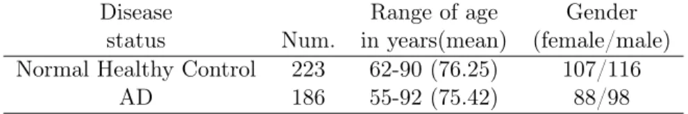
2.6.1 The ADNI Data . . . 74
2.6.2 Intrinsic Regression Model . . . 76
2.6.3 Results . . . 78
2.7 Discussion . . . 82
3 LONGITUDINAL DATA ANALYSIS ON RIEMAN-NIAN MANIFOLDS . . . 87
3.1 Introduction . . . 87
3.2 Intrinsic Regression Model . . . 89
3.2.1 Formulation of Intrinsic Fixed Effect Regression Model . . . 89
3.3 Longitudinal ADNI Corpus Callosum Shape Data Example . . . 92
3.3.1 Intrinsic Fixed Effects Model . . . 92
3.3.2 Results . . . 94
3.4 Simulation Study . . . 98
4.1 Introduction . . . 106
4.2 Time-Varying Agreement Measures . . . 109
4.3 Mixture Models for Estimating Time-Varying Agreements . . . 110
4.4 Observed Likelihood and Inference . . . 113
4.5 Simulation Study . . . 118
4.6 Head and Neck Cancer Trial . . . 121
4.7 Discussion . . . 128
5 CONCLUSIONS . . . 132
APPENDIX : TECHNICAL DETAILS FOR CHAPTER 2 . . . 136
A.1 Differential Geometry . . . 136
A.1.1 Technical Details . . . 136
A.1.2 Unit circle S1 in the complex plane . . . 148
A.1.3 Lie Logarithmic Maps of SO(2) and SO(3) . . . 149
A.2 Proofs for Chapter 2 . . . 153
A.3 RSS method versus more naïve approaches . . . 170
A.4 Annealing evolutionary stochastic approximation Monte Carlo . . . 172
LIST OF TABLES
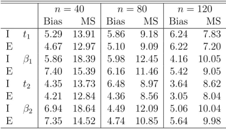
2.1 Bias (×10−3) and MS(×10−2) of (ˆt
I,βˆI) and (ˆtE,βˆE).
Bias denotes the bias of the mean of the estimates; MS
denotes the root-mean-square error. . . 72 2.2 Bias (×10−3), MS(×10−2), SD(×10−2), and RE of(ˆt
E,βˆE).
Bias denotes the bias of the mean of the estimates; MS denotes the root-mean-square error; SD denotes the mean of the standard deviation estimates; RE denotes the
rel-ative efficiency, which is the ratio of MS over SD. . . 72 2.3 Comparisons of the rejection rates for Wald test
statis-tics. Three different sample sizes n ∈ {40,80,120} and 2000 simulated datasets were used for each case and two
significance levels, 5% and 1%, were considered. . . 73 2.4 Demographic information about processed ADNI CC shape
dataset, including disease status, age, and gender. . . 76
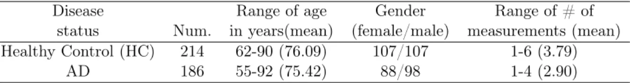
3.1 Demographic information about processed longitudinal ADNI CC shape dataset, including disease status, age,
gender, and number of measurements. . . 93 3.2 Bias (×10−2) and MS(×10−2) of (ˆt
I,βˆI) and (ˆtE,βˆE).
Bias denotes the bias of the mean of the estimates; MS
denotes the root-mean-square error. . . 99
4.1 Summary of simulation results from data with RC . . . 122 4.2 Summary of simulation results from data without RC . . . 123 4.3 True values, estimates, and biases of the weighted area under
the curve of the agreement measures pA and nA, and of Kendall’s coefficient of concordance τ, in both data with RC and without RC cases, for maximum follow-up times TE =
0.5,1.5,2.5,3.0, agreement probabilities p = 0.2,0.6,0.8, sample size n = 200, and all the other parameters as in
Tables 4.1 and 4.2. . . 124 4.4 Summary of simulation results for data from the distribution
described at the end of Section 4.5, for which the model is
4.5 Head and neck cancer trial data information at times
t = 0.5,1.5,2.5. (n= 89) . . . 126 4.6 Parameter estimates, standard deviations, and 95%
confi-dence intervals of the parameters for the head and neck
can-cer trial data. (sample size n= 89). . . 126 4.7 Estimated values, standard deviations, and 95% confidence
intervals of the agreement measurespAandnAfor the head
and neck cancer trial data.. . . 127 4.8 Estimated values of the weighted area under the agreement
measures pAandnA, and of the Kendall’s coefficient of
con-cordance τ for the head and neck cancer trial data. . . 127 A.1 Comparison of the performance of RSS model and naïve
LIST OF FIGURES
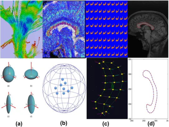
2.1 Examples of manifold-valued data: (a) diffusion tensors along white matter fiber bundles and their ellipsoid rep-resentations; (b) principal direction map of a selected slice and their directional representations on S2(1); (c)
median representations and median atoms; and (d) au-tomatic corpus callosum segmentation and its contour
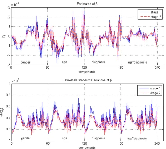
and landmarks of a selected subject. . . 36 2.2 Regression coefficient estimates and their standard
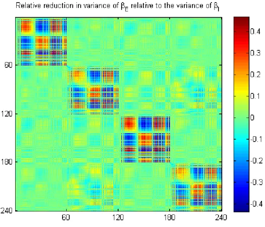
devia-tions from stage I and stage II. . . 79 2.3 The relative reduction in the variances-covariances ofβE
rel-ative to the to the variances ofβI. In average, there is about
a 16.77% relative decrease in variances in average; 12.25%
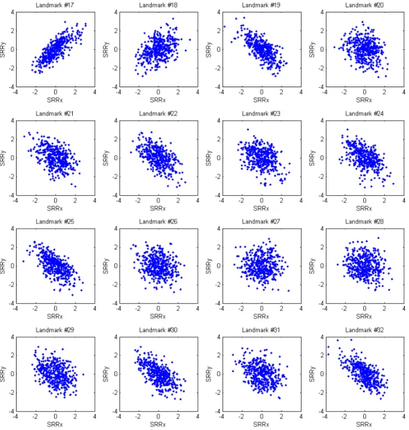
for β(ad) and 19.98%for β(g). . . 80 2.4 The plots of the rotated residuals at the first 16 landmarks . . . 84 2.5 The plots of the rotated residuals at the last 16 landmarks . . . 85 2.6 Age-trajectories of the intrinsic mean shapes by diagnosis
within each gender group, based on the stage II parameter estimates. . . 86 2.7 Age-trajectories of the intrinsic mean shapes by gender within
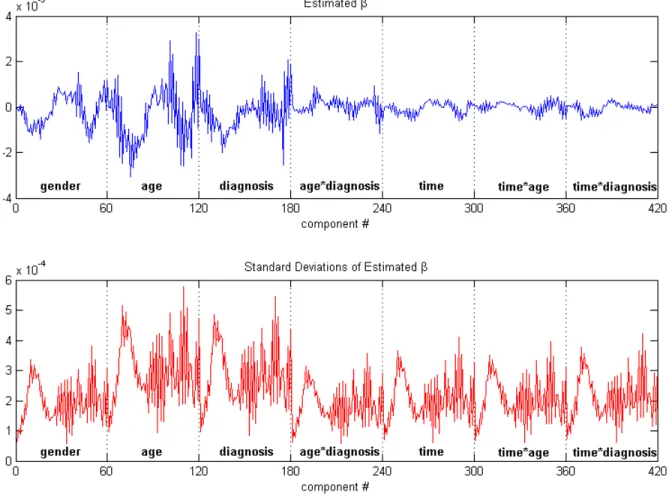
each diagnosis group, based on the stage II parameter estimates. . . 86 3.1 Longitudinal ADNI Date: Histogram of the number of measurements. . . 93 3.2 Longitudinal ADNI Data: Estimated regression coefficients
and their standard deviations. . . 95 3.3 Longitudinal ADNI Data: Estimated regression coefficients
and their standard deviations. . . 96 3.4 Longitudinal ADNI Data: The plots of the rotated residuals
at the first 16 landmarks . . . 100 3.5 Longitudinal ADNI Data: The plots of the rotated residuals
at the last 16 landmarks . . . 101 3.6 Top: Conditional mean trajectories of a 71-year old normal
HC female and her would-be AD counterpart subject. Bot-tom: The conditional mean and observed shapes at the
3.7 Top: Conditional mean trajectories of a 87-year old AD male and his would-be HC counterpart subject. Bottom: The
con-ditional mean and observed shapes at the measurement times. . . 103 3.8 Top: Conditional mean trajectories of a 71-year old normal
HC male and his would-be AD counterpart subject. Bottom:
The conditional mean and observed shapes at the
measure-ment times. . . 104 3.9 Longitudinal Simulation Study: Plots of the “true” and
es-timated fixed effect trajectories for a subject, based on the
longitudinal simulated data on S2. . . . 105
4.1 Plots of the curves of the agreement measures pA and
nA. Top: ρ = 0.5fixed andpvarying,p= 0, 0.2, 0.4, 0.6, 0.8, 1; bottom: p= 0.5fixed andρvarying,ρ= 0, 0.2,0.4, 0.6, 0.8; all other parameters being set to the values as in Tables
4.1 & 4.2, and TE = 3.0. . . 114
4.2 Plots of the areas, wAU C(pA) and wAU C(nA), under the agreement measure curves pA and nA, respectively,
and the Kendall’s coefficient of concordance τ. . . 115
4.3 Plots of the estimated curves of the agreement measures pA and nA, together with the pointwise 95% confidence bands, over the study duration for PFS data. The weighted AUCs
are wAU C(pA) = 0.412andwAU C(nA) = 0.843. . . 128 A.1 (a) A medial representation model m = (O, r,s0,s1) at an
atom, whereO is the center of the inscribed sphere,r is the common spoke length, abd {s0,s1} are the two unit spoke
directions; (b) a skeleton of a hippocampus with 24 medial
atoms,; (c) the smoothed surface of the hippocampus. . . 146 A.2 RSS model vs. naïve method: predicted responses an rotated
CHAPTER 1: LITERATURE REVIEW
We first review the literature on curved data in non-Euclidean spaces, such as differential manifolds. We then focus on the existing literature on agreement measures in bivariate time-to-event censored data.
1.1 Manifold-Valued Data
Statistical inference for distributions on manifolds is a broad discipline with wide ranging applications. Its study has gained momentum, due to its applications in bio-sciences and medicine, geobio-sciences, astronomy, computer vision and image analysis, electrical engineering, and other fields.
Statisticians are working more and more with nonlinear object data, regarding the observations as points on manifolds. The idea of a data analysis on abstract metric space goes back to a visionary paper by Fréchet (1948), where he suggested to analyze object data on separable metric spaces rather than just on linear spaces in an effort to accommodate a large variety ofelements (objects) that need to be analyzed statistically. Fréchet’s ideas got exploited much later, especially with the increase of compu-tational capabilities, so that his approach could be followed numerically. The first examples of data analysis on manifolds are due to Watson (1983), for directional data analysis (on spheres and real projective spaces), to Kendall (1984a), for similarity shape data analysis (on complex projective spaces), and to Chang (1988), for tectonic plates data analysis (on groups of rotations).
(2000), Stiefel manifolds - Hendriks and Landsman (1998), projective shape manifolds (product of real projective spaces) - Patrangenaru (2001), or on affine shape manifolds (Grassmannians) - Patrangenaru and Mardia (2003).
The common features of all these sample spaces are reflected in the fact that they are all homogeneous spaces. Given data in a homogeneous space to be analyzed, it is statistician’s choice of selecting an appropriate Riemannian structure on the sample space, that would best address the data analysis.
In the areas of directional data analysis or shape data analysis that dominated object data analysis in its initial phase, the homogeneous spaces considered as sample spaces were compact spaces. In recent years, the attention has turned to brain imaging data and size-and-shape data analysis in structural genomics for which the sample spaces considered are noncompact (see Bandulasiri et al. (2009a) and Bandulasiri et al. (2009b)). One object of our research is to develop a unified framework for data analysis on compact and noncompact Riemanian homogeneous spaces.
Statistical analysis on general homogeneous spaces was first considered in the con-text of density estimation with the pioneering paper by Beran (1968). This line of research was also pursued for function estimation on Lie groups via Fourier analysis by Kim (1998; 2000), Lesosky et al. (2008), and Koo and Kim (2008a). Such method-ologies found applications in medical imaging, robotics, and polymer science (Yarman and Yazici (2003; 2005), Koo and Kim (2008b)).
Data analysis of data taking values in an homogeneous spaces that admit a non-compact Riemannian structure appeared first in Diffusion Tensor Imaging (DTI) and inCosmic Microwave Background (CMB) radiation (Schwartzman et al. 2008b). Both areas lead to analysis of random objects on the set of symmetric positive definite ma-trices Sym+(m). The main statistical techniques used for DTI data were parametric
(2011), Osborne and Patrangenaru (2011), Osborne (2012), Zhu et al. (2009a), Yuan et al. (2012a), Yuan et al. (2012b), and Shi et al. (2012) used the geometric approach of Lie group action, which is related to the approach in our research.
Data belonging to some m-dimensional compact submanifold M of Euclidean space
RN appear in many areas of natural sciences. Directional statistics, image analysis,
vector cardiography in medicine, orientational statistics, plate tectonics, astronomy, and shape analysis comprise a (by no means exhaustive) list of examples. Research in the statistical analysis of such data is well documented in the pioneering book by Mardia (1972) and more recently in the book by Mardia and Jupp (2000). In these books, as well as in many research papers , the primary emphasis is placed on the analysis of data on a circle or a sphereSd. These are the simplest examples of compact
manifolds and do not manifest the generic features of statistical inference intrinsic to compact submanifolds of Euclidean spaces.
There is an immense literature that has been devoted to shape representation, shape descriptors, or shape signatures in computer vision. An overview of several shape space models with Riemannian manifold structure, including some shape representation methods, shape spaces structures (from metric spaces to manifolds), and applications that result from such models, is given in Younes (2010). There are many ways to define the notion of shape. To simplify, a shape can be interpreted as the boundary of a two-or three-dimensional object. A shape representation is a function that assigns to a given shape a well-defined mathematical feature that will simplify further algorithms and analysis. For example, the shape of an m-dimensional object is represented by k > m points in Rm called landmarks, which represent k locations on an object. The
configuration of k landmarks is called a k-ad. The choice of landmarks is generally
a group of transformations. For example, one may look at k-ads modulo size and
Euclidean rigid body motions of translation and rotation. The analysis of shapes under this invariance was pioneered by Kendall (1977; 1984b) and Bookstein (1978). Kendall identified a shape with the orbit under m-dimensional rotations of a k-ad centered at
the origin and scaled to have unit size. The resulting shape spaces are called similarity shape spaces, or Kendall’s shape space, and denoted by Σkm. A fairly comprehensive account of parametric inference on these spaces, with many references to the literature, may be found in Dryden and Mardia (1998). When the orbits are considered under all orthogonal transformations and scaling, the resulting shape spaces are called reflection shape spaces and denoted by RΣk
m. A computation of the extrinsic mean reflection
shape, which has remained unresolved in earlier works, was given by Bhattacharya (2008) in arbitrary dimensions, enabling one to extend nonparametric inference on Kendall type shape manifolds from 2D to higher dimensions.
Data belonging to noncompact submanifold M appears in many applications
in-cluding Diffusion Tensor Imaging (DTI), Cosmic Microwave Background radiation (Schwartzman et al. 2008b), medical imaging, brain imaging (Zhu et al. 2009a, Os-borne and Patrangenaru 2011, Ellingson et al. 2012), structural genomics (Bandulasiri et al. 2009a;b), computational anatomy, and statistics. A specific such a manifold is the space Sym+(m) of m×m symmetric positive-definite (SPD) matrices defined as
follows.
Sym+(m) = {S ∈Sym(m) : x>Sx>0, for all nonzerox∈Rm},
where Sym(m) ⊂M(m,R) denote the linear space of all m×m symmetric matrices,
and M(m,R) is the space of all m×m matrices with real entries.
of manifold-valued response in a Riemannian symmetric space (RSS) and its relation-ship with covariates of interest, such as age, in Euclidean space. Such manifold-valued data, such as directional data and symmetric positive-definite matrices, arises frequently in medical imaging, computational biology, molecular imaging, surface modeling, and computer vision, among many others. However, little has been done when the response is in a general RSS. We develop an intrinsic regression model solely based on an intrinsic conditional moment assumption, avoiding specifying any parametric distribution in RS space. We propose various link functions to map from the Euclidean space of covari-ates to the the RS space of responses. We develop a two-stage procedure to calculate the parameter estimates, and determine their asymptotic distributions. We construct the Wald and geodesic test statistics to test hypotheses on unknown parameters. Sim-ulations studies are used to evaluate the finite sample property of our methods and a real data set from Alzheimer’s Disease Neuroimaging Initiative (ADNI) database is analyzed to illustrate the use of our test statistics.
1.2 Statistical Analysis of Manifold-Valued Data in the Literature
1.2.1 Fréchet Mean Set
The earliest literature on statistical analysis on spaces other than Euclidean ones goes back to mid 20-th century, when Fréchet (1948) introduced the notion of the mean for a distribution on a metric space (M, d). Let Q be a probability distribution
on(M, d), i.e. on the Borel σ-algebra ofM.
Definition 1.2.1. The Fréchet mean set of Q, denoted CQ, is the set of all minimizers
of the Fréchet function F on M defined by
F(p) = ˆ
M
assuming thatF(p)<∞for some p∈M. If there is a unique minimizer, say µF, then
CQ ={µF} and µF is called the Fréchet mean of Q.
The Fréchet mean set CQ is a natural index of location for the probability
distribu-tion Q.
Since their original definition as metrical means by Fréchet in 1948 such means have found much interest. Independently, on Riemannian manifolds with respect to the Riemannian metric, Kobayashi and Nomizu (1996) defined the corresponding metrical means in the original space as centers of gravity. With application in landmark based shape analysis in mind, Ziezold (1977) extended the concept to quasi-metrical means (in the sense that the distance function d : M ×M → [0,∞) is not required to be symmetric). Further generalizations can be found in Huckemann (2011).
Applications of this concept for data analysis did not get too much traction until it could have been followed numerically. Due to the high computational complexity on the manifolds, it was not before mid-late 1980s when data analyses on manifolds were performed.
The concept of variation was introduced in Bhattacharya and Patrangenaru (2002), where it has been referred to as the total variance, as the minimum value of F on M.
It is called theFréchet variation of Q and denoted by V.
Definition 1.2.2. If Y1, Y2, ..., Yn are independent and identically distributed (iid) M
-valued random variables defined on some probability space (Ω,F,P) with common dis-tribution Q, and Qˆn := 1/n Pni=1δYi is the corresponding empirical distribution, then the Fréchet mean set of Qˆn is called the sample Fréchet mean set, denoted byCQˆn. The
Fréchet variation of Qˆn is called the sample Fréchet variation and denoted by Vˆn.
is nonempty, as proved by Bhattacharya and Patrangenaru (2003) and Bhattacharya (2008).
Proposition 1.2.1. Suppose(M, d)is a metric space such that every closed and bounded subset of M is compact (the Heine-Borel property). If the Fréchet function F of Q is finite for some p∈M, then CQ is nonempty and compact.
Consistency of the Fréchet mean set. An important question on estimation of loca-tion is that of consistency. Two different Strong-Consistency results for Fréchet sample means have been obtained by Ziezold (1977), Theorem I, for quasi-metrical means on separable spaces (i.e. containing a dense countable subset) and by Bhattacharya and Patrangenaru (2003), Theorem 2.3, for metrical means on spaces with Heine-Borel property (i.e. that every closed bounded set is compact).
Theorem 1.2.1. (Strong Consistency - Ziezold (1977)) Let (Ω,F,P) be a probability space and (M, d) a separable quasi-metric space. Let Y1, Y2, . . . be independent,
identi-cally distributed random M-valued variables, Yi : Ω → M, i = 1,2, . . ., with common
distribution Q, such that F(p)<∞ for some p∈M. Then for almost all ω∈Ω
∞
\
n=1
∞
[
k=n
CQk(ω) ⊆CQ,
where A denotes the closure of the set A.
Theorem 1.2.2. (Uniform Strong Consistency - Bhattacharya and Patrangenaru (2003)) Let (Ω,F,P) be a probability space and (M, d) a metric space such that every closed and bounded subset of M is compact (the Heine-Borel property). Let Y1, Y2, . . . be
inde-pendent, identically distributed random M-valued variables, Yi : Ω→ M, i = 1,2, . . .,
ε >0 and almost all ω∈Ω, there exist a number N =N(ε, ω) such that ∞
[
k=N
CQˆk(ω)⊆ {p∈M :d(CQ,p)≤ε}.
In particular, if CQ={µF}, then the sample Fréchet mean µFn (any measurable selec-tion from CQˆn) is a strongly consistent estimator of µF.
Bhattacharya and Patrangenaru, 2003„ in Remark 2.5, note that Ziezold’s strong-consistency implies theirs for compact metric spaces M, but not for noncompactM.
The following strong consistency ofVˆ
n as an estimator ofV is due to Bhattacharya
and Bhattacharya (2008).
Theorem 1.2.3. Suppose(M, d) is a metric space with Heine-Borel property andF is finite on M. Then Vˆn is a strongly consistent estimator of V .
Asymptotic theories for the Fréchet means on manifolds was established in Bhat-tacharya and Patrangenaru (2003; 2005) and Huckemann (2011).
Central Limit Theorems. The ”δ-method” allows to formulate Central-Limit
Theo-rems (CLTs) for differentiable images of random variables. The following definition of CTL for random manifold-valued variables was given in Huckemann (2011).
Definition 1.2.3. Let M be a smooth m-dimensional manifold. We say that a M -valued estimator µn(ω) of µ ∈ M satisfies a Central-Limit-Theorem (CLT), if in any
local chart (U, φ) near µ there is a suitable m×m matrix Aφ and a m×m positive
semi-definite symmetric matrix Σφ such that
√
n Aφ(φ(µn)−φ(µ)) d
→Nm(0,Σφ)
In most applications Aφ is non-singular, then as a consequence of the ”δ-method”,
for any other chart (U0, φ0) near µ, we have
A−φ01Σφ0 A−1 φ0
>
=J(φ0◦φ−1)φ(µ)A−φ1Σφ A−φ1 >
J(φ0◦φ−1)>φ(µ)
whereJ(·)a denotes the Jacobi-matrix of the first order derivatives at a.
Suppose now that d is a metric on a differentiable manifold M, and p→ d(q,p)is at least twice continuously differentiable on M, for any q ∈ M. We can only expect a
CLT for the Fréchet mean set to hold under additional regularity conditions concerning the expectation of derivatives of d. To this end, in a local chart (U, φ) on M, denote
by grad2d(q,p)2 the gradient of u → d2(q, φ−1(u)) at u = φ−1(p) for p ∈ U, and Hess2d(q,p)2 the corresponding Hessian matrix of the second order derivatives. We
mention here two CLT results.
First, Bhattacharya and Patrangenaru (2005) establish a CLT when there is a unique Fréchet meanµF of Q and there is a local (U, φ)that almost covers M, i.e. Q(U) = 1.
Theorem 1.2.4. (CLT for Fréchet means - Bhattacharya and Patrangenaru (2005)) Let Q be a probability measure on a differentiable manifold M endowed with a metric
d(·,·) such that (M, d) has the Heine-Borel property. Let Yi, i = 1,2, . . ., be i.i.d.
random variables onM with common distributionQ, and µn,F be a measurable selection
from the Fréchet mean set (w.r.t. d) of the empirical Qˆn = n1 Pni=1δYi. Assume
(i) the Fréchet mean µF exists,
(ii) there exists a local chart (U, φ) such that Q(U) = 1,
(iii) the map u→d2(q, φ−1(u)) is twice differentiable onφ(U),
(iv) EQ(kgrad2d(Y1, µF)2k2)<∞, EQ
(Hess2d(Y1, µF) 2)
k,l
2
(v) EQ sup p :d(p,µF)<ε
(Hess2d(Y1,p) 2)
k,l−(Hess2d(Y1, µF)2)k,l
!
→ 0 as ε → 0, k, l = 1, . . . , m.
Then,
(a) µn,F is a consistent estimator of µF, and
(b) √nAφ(φ(µn,F)−φ(µF)) d
→Nm(0,Σφ),
with
Aφ =EQ(Hess2d(Y1,p)2) and Σφ = Cov(grad2d(Y1, µF)2). (1.1)
The assumption above on the existence of a local chart (U, φ) such that Q(U) = 1 is less restrictive than it may seem. If m is a Riemannian structure on M and Q is
absolutely continuous with respect to the volume measure, then, for any given p∈M,
the complement U of the cut locus C(p), is the domain of definition of such a local chart, φ = Logp, the Riemannian logarithmic map of M at p. For example, when M =Sm, the unit sphere in Rm+1 with the canonical Riemanian structure, for a given
p ∈ Sm, the maximal normal chart centered at p is given by U = Sm \ {−p} and
φ(y) =Logp(y) = (y−(p>y)p)arccos(p>y)/p1−(p>y)2. Any probability measureQ
onSm that has no mass concentrated at −p satisfiesQ(U) = 1.
Second, the most general CLT result to date is due to Huckemann (2011). The so-called Fréchetρ-mean set of a probability distribution Qon M is defined in a more
general setting, where the distancedis replaced by a continuous functionρ:M×P → [0,∞), whereM is a topological space and(P, dP)is aspace with distance(in the sense
thatP is a topological space anddP :P×P →[0,∞)is a continuous map that vanishes
on the diagonal {(p, p) : p ∈ P}). Fréchet ρ-mean set of Q is a subset of P. In this
second argument uniform over the first argument, and (c2) a version of coercivity in the second argument: there are p0 ∈P and C >0 such that Pr(ρ(Y, p0)< C)>0, for
Y ∼Q, and that such that for every sequence pn ∈ P with dP(p0, pn)→ ∞ there is a
sequence Kn → ∞ with ρ(y, pn) > Kn for all y ∈ M with ρ(y, p0) < C; moreover, if
pn ∈P with dP(p∗, pn)→ ∞ for some p∗ ∈ P, then dP(p0, pn) → ∞. Both properties
are valid if M = P and ρ is a quasi-metric. Huckemann showed that property (c1)
implies the strong consistency, assuming that the Fréchet function is finite at least at one point inP (Theorem 3.4 in Huckemann (2011)). He also showed that, when P
enjoys the Heine-Borel property and the Fréchetρ-mean set is nonempty, the conditions
(c1) and (c2) together imply uniform strong consistency (Theorem 3.5 in Huckemann (2011)). It may be pointed out that it is the assumption of some symmetries of P
that often causes the Fréchet ρ-mean set to contain more than one element (see, e.g.,
Proposition 2.2 in Bhattacharya and Patrangenaru (2005)). This situation is taken care of too in Huckemann’s CLT result as follows.
Theorem 1.2.5. (CLT - Theorem 3.8 in Huckemann (2011)) Assume P =R, whereR
is a smooth manifold, and there is a self-understood discrete groupHacting smoothly on
R such that{p0 ∈R : dR(p, p0) = 0}={hp : h∈H}, for any p∈R. Suppose thatµis
a point in the Fréchet ρ-mean set unique up to the action of H on the manifold R (i.e. Fréchet ρ-mean set equals Hµ) with respect to a continuous ρ : M ×R → [0,∞), ρ2
smooth in the second argument, satisfying uniform consistency, whereM is a topological space. Let Yi, i = 1,2, . . ., be i.i.d. random variables on M with common distribution
Q. If
(i) probability measure Q on M has compact support or
(ii) in a suitable local chart on R near µ, EQ(grad2ρ(Y1, µ)2) exists,
CovQ(grad2ρ(Y1, µ)2) exists, and EQ(Hess2ρ(Y1, ν)2) exists for ν near µ and is
then for any measurable choice µo
n in the sample Fréchetρ-mean set there is a sequence
hn ∈ H such that µn = hnµon satisfies a CLT. In a suitable local chart (U, φ) on R
near µ the corresponding matrices in CLT are given by Aφ = EQ(Hess2ρ(Y1, µ)2) and
Σφ =CovQ(grad2ρ(Y1, µ)2).
1.2.2 Intrinsic and Extrinsic Mean Sets
IfM is a Riemannian manifold, the Fréchet mean (set) with respect to the geodesic
distance d = dm is defined to be the intrinsic mean (set) of Q and denoted µI(Q).
The corresponding Fréchet variation is called the intrinsic variation of Q and denoted VI(Q).
In the case of M is connected C∞ Riemannian manifold with a metric tensor m
and geodesic distancedm, with(M, dm)a complete metric space, Theorem 2.1 in Bhat-tacharya and Patrangenaru (2003) shows that (i) the intrinsic Fréchet mean set is compact, (ii) for each point µ in the intrinsic mean set, the Euclidean mean of the of
the distribution on the tangent space at µ of the Riemanian logarithmic map is zero,
and (iii) in the case of simply connectedM of nonpositive curvature, the intrinsic mean
exists if F(·) is finite. A particular case of this result, when M is a Bookstein’s shape
space of labeled triangles, with Riemannian metric of constant negative curvature is due to Le and Kume (2000). From a result of Karcher (1977) it follows that if the distribution is sufficiently concentrated then the intrinsic mean exists. For complete Riemannian manifolds, it seems that the sharpest uniqueness result to date for the intrinsic mean is due to Afsari (2011): if Q is supported in a ball of radius less than the geodesic convexity radius of (M,m), then the minimizer of FQ (for d = dm) is
unique. For planar shape space CPk−2, a useful necessary and sufficient condition for
the existence of an intrinsic mean is proved by Le (1998) for distributionsQ which are
function only of the distance from a given point.
Much of the literature in the field deals with special cases of what it is calledextrinsic mean, perhaps because of the difficulties involved in proving the existence of an intrinsic mean and in computing the intrinsic sample mean, even when it exists. It is simpler both mathematically and computationally to carry out an extrinsic analysis on M, by
embedding it into some Euclidean spaceRN via some mapJ :M →RN such that both
J and its derivative are injective, and for which J(M) has the induced topology from
RN. ThenJ induces the metricd
J(x, y) = kJ(x)−J(y)kRN onM, wherek·kRN denotes Euclidean norm (kuk2
RN =
PN i=1u
2
i, for any u = (u1, u2, ..., uN)>). This is called the
extrinsic distance on M. Among the possible embeddings, one seeks out equivariant embeddings which preserve many of the geometric features of M. For a Lie group H
acting on a manifold M, an embedding J :M →RN isH-equivariant, if there exists a group homomorphism ϕ:H → GL(N,R) such that J(a·p) =ϕ(a)J(p) for all p∈M
and all a ∈ H. Here, GL(N,R) is the general linear group of all N ×N non-singular
matrices. The extrinsic mean and variations of a probability distribution Q on M are
defined (see below) with respect to the embedding J. The notion of extrinsic mean
on a manifold was introduced independently by Hendriks and Landsman (1998) and Patrangenaru (1998), and later considered in detail in Bhattacharya and Patrangenaru (2003; 2005).
The Fréchet mean set of Q with respect to the distance dJ is called the extrinsic
mean setofQand the Fréchet variation ofQis called theextrinsic variationof Q. IfYi,
i= 1, . . . , n, are iid observations fromQ, then the Fréchet mean set ofQˆn is called the
sample extrinsic mean setand the Fréchet variation ofQˆnis called the sample extrinsic
variation.
In case J(M) = ˜M is a closed subset of RN, for every u ∈ RN, there exists a
˜
M. This set is the set of projections of u on M˜ and denote it by PM˜(u) ={x ∈ M˜ :
kx−ukRN ≤ ky−ukRN for any y ∈ M˜}. If this set is a singleton, u is said to be a nonfocal point of RN (with respect to M˜), otherwise it is said to be a focal point of RN.
For a given embedding J, Bhattacharya and Patrangenaru (2003) established the
relationships between the extrinsic mean and variation of Q on M and the mean and
variation of the push forward probability distributionQ˜ =Q◦J−1 ofQontoRN. They
showed that the extrinsic mean set ofQ is given by J−1(P ˜
M(˜µ)), where µ˜ is the mean
of Q˜, and the extrinsic variation ofQ is given by
V = ˆ
RN
kx−µ˜k2Q˜(dx) +kµ˜−µk2,
whereµ∈PM˜(˜µ).
An asymptotic theory for the intrinsic and extrinsic means on manifolds was es-tablished in Bhattacharya and Patrangenaru (2003; 2005). Asymptotic distributions of extrinsic sample means were derived. Explicit computations of these means of Q˜
n and
their asymptotic dispersions were carried out for distributions on the sphereSd
(direc-tional spaces), real projective space RPN−1 (axial spaces), and CPk−2 (planar shape
spaces). Nonparametric inference procedures for estimation and testing problems for sample Fréchet means on manifolds were also derived and bootstrap methods for these problems were presented, with applications to distributions on Sd, RPN−1, CPk−2
with respect to Veronese-Whitney embeddings, and a 3-dimensional shape spaceΣ4 3. A
detailed theory of shape-spaces Σk
m can be found in the pioneering paper by Kendall
(1984b), and a brief description of these spaces is presented below.
Central Limit Theorems for Intrinsic Means. In the case Q is a probability
distri-bution onM whose support is compact and is contained in a local chart, an immediate
Corollary 1.2.1. Let (M,m) be a m-dimensional Riemannian manifold and d =dm
be the geodesic distance. Let Q be a probability distribution on M whose support is compact and is contained in a local chart(U, φ). Assume that (i) the intrinsic meanµI
exists, (ii) the map u → d2(q, φ−1(u)) is twice continuously differentiable on φ(U) for
each q ∈U and Aφ and Σφ defined as in (1.1). Then the conclusion of Theorem 1.2.4
holds for the intrinsic sample mean µn,I.
Two main CLT results for intrinsic means are established by Bhattacharya and Patrangenaru (2005). One is relative to normal charts on M when the support of Q
is in a geodesically convex ball whose radius depends on the sectional curvature of M,
and the second when the uniqueness of the intrinsic mean is assumed. The other allows for multiple intrinsic means due to the invariance of Qunder a group of symmetries.
Theorem 1.2.6. Let(M,m)be a Riemannian manifold and letd=dm be the geodesic
distance. Let Q be a probability measure on M whose support is contained in a closed geodesic ball Br = Br(p0) with center p0 and radius r which is disjoint from the cut
locus C(p0). Assume r < 4Kπ , where K2 is the supremum of the sectional curvatures in
Br if this supremum is positive, or zero if this supremum is nonpositive. Then
(a) the intrinsic mean µI (of Q) exists, and
(b) then the CLT from the conclusion of Theorem 1.2.4 holds for any measurable intrinsic sample meanµn,I ofQˆn = n1
Pn
i=1δYi, under the normal chartφ= Logp0. We note here, that if the supremum of the sectional curvatures (of a complete manifoldM) is nonpositive, and support of Qis contained in Br, for some r >0, then
the hypotheses of Theorem 1.2.6 are satisfied, and the conclusions (a) and (b) hold. One may apply this theorem even with r=∞.
The assumptions in Theorem 1.2.6 on the support of Q for the existence of µI are
be entirely dispensed with, as can be shown by lettingQbe the uniform distribution on
the equator of S2. For example, as it was mentioned above, Le (1998) gives necessary
and sufficient conditions for the existence of the intrinsic mean µI of an absolutely
continuous (w.r.t to the volume measure)Qon the projective spaceCPk−2,k ≥3, with radially symmetric density. The standard Riemannian structure on CPk−2 is induced
by the circular arc metric, i.e. the geodesic distancedis given bycos(d([ζ],[ξ])) =|ζ>ξ|, whereζ = (ζ1, . . . , ζk−1)>,ξ = (ξ1, . . . , ξk−1)>∈Ck−1, withPi|ζi|2 =Pi|ξi|2 = 1. Let
f([ζ])be the density function of Q with respect to the volume measuredω on Ck−2. If
f(·) can be expressed as a non-increasing function of the distanced of [ζ] from a fixed point[µ] and is strictly decreasing on a set of positive measure, then[µ]is the unique intrinsic Fréchet mean of Q.
Thus, assuming the that the intrinsic mean is unique, the following result may be more generally applicable than Theorem 1.2.6.
Theorem 1.2.7. (CLT - Theorem 2.3 in Bhattacharya and Patrangenaru (2005)) Let
Q be absolutely continuous with respect to the volume measure on a Riemannian man-ifold (M,m). Assume that µI is exists, the integrability conditions (iv) in Theorem
1.2.4 hold, the Hessian matrix Aφ of the Fréchet function F with respect to a local
chart φ near µI is is nonsingular, and the covariance matrix Σφ of the grad2d(Y1, µI)2
is nonsingular. Then √n(φ(µn)−φ(µI)) d
→N(0, A−φ1ΣφA−>φ ).
1.3 Longitudinal Data on Manifolds
a different shape, whereas its maturation may follow some common patterns that one would like precisely to describe and quantify. The computational anatomy, an emerging discipline at the interface of geometry, statistics and image analysis, aims at modeling and analyzing the biological shape of tissues and organs. The goal is to estimate representative organ anatomies across diseases, populations, species or ages, to model the organ development across time (growth or aging), to establish their variability, and to correlate this variability information with other functional, genetic or structural information. In clinical studies, one wants to characterize anatomical or functional changes due to disease progression, clinical intervention or therapy. In cardiac imaging, one looks for abnormal patterns in the heart motion. What make these questions so challenging is the nature of the object of interest and that it changes in appearance in different situations. The observed object’s features, such as the shape, are is inherently nonlinear and high-dimensional. Because of this, manifold representations of the data have proven to be effective. These problems can be addressed by statistical analysis of longitudinal data that takes values in a Riemannian manifold. The Riemannian structure provides useful tools to carry out such analyzes.
called “template” or “atlas”. The extension of these concepts for longitudinal shape data is challenging, as there is no consensus about how to combine shape changes over time and shape changes across subjects.
There has been extensive research for the analysis of Euclidean longitudinal data in the last few decades. Diggle et al. (2002) and Fitzmaurice et al. (2008) provided a comprehensive overview of various models and methods for the analysis of longitudinal data, among others. In the analysis of longitudinal data, three types of models are commonly used: mixed effects models, GEE models, and transitional models.
Recent work suggests that attempts to describe anatomical shapes using flat Eu-clidean spaces undermines our ability to represent natural biological variability (Fletcher et al. 2004a, Grenander and Miller 1998).
A number of longitudinal growth models have been developed to provide this type of analysis to time-series imagery of a single subject (e.g., Beg (2004); Clatz et al. (2005), Miller (2004); Thompson et al. (2000)). While these methods provide important results, their use is limited by their reliance on longitudinal data, which can be impractical to obtain for many medical studies. Also, while these methods allow for the study of an individualâĂŹs anatomy over time, they do not apply when the average growth for a population is of interest.
difficult to compare the differences in trends of two groups, or even to rigorously define the concept of the variance of a population of trends.
The aim of this research is to extended our framework of intrinsic regression models for cross-sectional data to fixed and random effect models for the analysis of manifold-valued measures from longitudinal studies.
1.4 Agreement Assessment in Bivariate Time-to-Event Times: Motivation Assessing agreement is often of interest in clinical studies and biomedical sciences to evaluate the similarity of measurements produced by different methods on the same subjects. For examples, when a new assay or instrument is developed, it is important to assess whether the new assay or instrument can reproduce the results of a traditional method. Additionally, the strength of agreement can help researchers decide whether a simple measurement is an acceptable replacement for a more expensive gold standard method and whether measurements obtained by different methods or instruments are comparable or not. Given the importance of agreement studies in biomedical sciences, there has been extensive literature on measuring agreement for categorical and contin-uous outcomes, e.g. Cohen (1960; 1968), Kraemer (1980), Kraemer et al. (2002), Lin (1989; 2000) among others.
censored observations.
Censoring is an issue complicating the assessment of reliability of time to event data. The presence of censoring raises problems in the application of commonly used measures of reliability or reproducibility. The nature of censoring depends on the study design. Right censored data can be produced in follow up studies if no event is reported by the time the study ends or if a subject drops out. Left-censored data may occur, for example, in a study of age-of-onset when subjects of varying ages are diagnosed as having the disease at baseline but no information is available on age of onset. In such studies, age-of-onset is censored by baseline age.
There are several agreement measures for assessing dependence or agreement for censored bivariate time-to-event data in the literature. The rank-based Kendall’s co-efficient of concordance τ (Section 4.2, Hougaard (2000)) is a measure of overall
de-pendence. It is simple and can be estimated non-parametrically for censored data, but does not measure the degree of agreement at a single time point. In the aforementioned extreme case, the data achieves the maximum value of Kendall’s τ, even that there is
no agreement of PD time at all. Liu et al. (2005) provided an estimation method of the concordance correlation coefficient for time-to-event data. It is a correlation type of measure and has the same issue as Kendall’sτ. Guo and Manatunga (2009) proposed
Our research in this area is motivated by a small phase 2 head and neck cancer trial. Progression-free survival (PFS), the time from ramdomization until disease progression (PD) or death, is a key endpoint to support licensing approval. The PD is determined by the investigator (local assessment), and also assessed by an independent review committee (IRC) blinded to the study (central assessment). Among a random subset of 92 subjects followed-up in the trial, the local assessment yields 82 local PFS events while the central assessment gives 72 events and the number of agreed events is 35. We propose a new method to assess temporal agreement between two time-to-event endpoints, where the two event times are assumed to have a positive probability of being identical. This method measures agreement in terms of the two event times being identical at a given time or both being greater than a given time. Overall scores of agreement over a period of time are also proposed.
1.5 Agreement Assessment in Bivariate Time-to-Event Times: Background
1.5.1 Bivariate Dependence Measures Correlation coefficient
A traditional way of evaluating dependence in a bivariate distribution is by means of the correlation coefficient (Pearson correlation), defined as
ρ(T1, T2) = Cov
(T1, T2)
[Var(T1)Var(T2)]1/2
.
The correlation is undefined when the variances in the denominator are 0 or infi-nite. An alternative expression based on the bivariate survivor function, S(t1, t2) =
P r(T1 > t1, T2 > t2) is Cov(T1, T2) =
´∞
0
´∞
0 [S(t1, t2) −S1(t1)S2(t2)]dt1dt2, where
S1(t1) = S(t1,0) and S2(t2) = S(0, t2) are the marginal survival functions. Similarly,
in the denominator the variance can be expressed as Var(T1) = 2
´∞
0
´∞
´∞
0 S1(t)dt 2
. The properties of the measure ρ(T1, T2) are that the range is [−1,1],
with the values±1if and only ifT1 andT2 depend linearly each other, i.e. T2 =a+bT1,
in which case ρ = 1 for b > 0 and −1 for b < 0. When T1 and T2 are independent,
then ρ = 0. In general, the reverse statement is not true. However, a value of 0 for ρ
implies that there is no linear correlation between the variables. More generally, note that (Ti1 −T¯1)(Ti2 −T¯2) is positive if and only if Ti1 and Ti2 lie on the same side of
their respective means. Thus the correlation coefficient is positive if Ti1 and Ti2 tend
to be simultaneously greater than, or simultaneously less than, their respective means. The correlation coefficient is negative if Ti1 and Ti2 tend to lie on opposite sides of
their respective means. The measure ρ is symmetric and invariant under linear
trans-formations, that is, ρ(T1, T2) = ρ(T2, T1) and ρ(T1, a+bT2) = ρ(T1, T2) for any a, b,
with b >0. In addition, it is L2-continuous, in the sense thatρ(Tn,1, Tn,2)→ρ(T2, T1),
if Tn,1 L2
→ T1 and Tn,2 L2
→ T2, as n → ∞. For normally distributed random variable,
the correlation coefficient is intimately related to the conditional distributions. The conditional mean and variance are
E[T2|T1] = E[T2]−ρ{Var(T2)/Var(T1)}1/2{T −1−E[T1]},
Var(T2|T1) = 1−ρ2Var(T2).
The correlation is very well suited for measuring the linear dependence in the bivariate normal distribution.
The estimation of ρ with complete data is straightforward, just substitute the
em-pirical mean and variances into the defining equation, i.e.
ˆ ρ=
Pn
i=1(Ti1−T¯1)(Ti2 −T¯2)
{[Pni=1(Ti1−T¯1)2][ Pn
The properties of this estimate are well known, when the distribution is bivariate nor-mal, but it is not known too much for general distributions.
Kendall’s Coefficient of Concordance
Another popular dependence measure is Kendall’s coefficient concordance which is defined as a rank-based correlation type measure. It was suggested first by Fechner in 1897 and later rediscovered by Kendall in 1938, who examined it more completely. It is a simple measure of concordance, which does not require the assumption of normality. For a set ofnindependent observed values(Ti1, Ti2),i= 1, . . . , n, of a bivariate variable
(T1, T2), τ is defined as
τ =E{sign[(T11−T21)(T12−T22)]},
where sign(x) is the sign of x, −1 for x < 0, 0 for x = 0, and 1 for x > 0. A more transparent formulation for continuous failure times is τ = 2p− 1, where p is the
probability that in two pairs the order of the first coordinates is the same as the order of the second coordinates, i.e. p=P r[(T11−T21)(T12−T22)>0]. Kendall’s τ has the
same nice properties as the correlation coefficient and in addition τ is unchanged by
both linear and nonlinear monotonic transformations. If the agreement between the two rankings is perfect (i.e. the two rankings are the same), then the coefficientτ has
value1. If the disagreement between the two rankings is perfect (i.e. one ranking is the reverse of the other), then the coefficientτ has value −1. If T1 and T2 are independent,
then τ = 0.
Alternatively, τ can be evaluated by integration of the bivariate survivor function,
τ = 4 ¨
For bivariate normal distribution, τ = 2 sin−1(ρ)/π, where ρ is the correlation
coeffi-cient.
Kendall’s concordance coefficient can be estimated non-parametrically for complete data, by considering each combination of two pairs, scoring each concordant pair as 1, each discordant pair as−1, and each tie as 0. This is then normalized in a similar way as a standard deviation. In the case of complete data, for each pair i and i0, let set aii0 =sign(Ti1 −Ti01) and bii0 =sign(Ti2−Ti02), i, i0 = 1, . . . , n. the sores for the first
coordinate and second coordinate, respectively. Then, the estimation formula is
ˆ
τ = 1
n(n−1)
n X
i,i0=1;i6=i0
aii0bii0,
for data without ties, and
ˆ τ =
n P
i,i0=1;i6=i0
aii0bii0
[(
n P
i,i0=1;i6=i0
a2 ii0)(
n P
i,i0=1;i6=i0
b2 ii0)]1/2
.
for data with ties.
In the case of ties or censored data, the latter formula can be used with the scoresaii0
andbii0 modified to account for censoring. A first suggestion is to use a score (a, b)of0
estimate. The values for thea scores are
aij = δi1δi01sign(Ti1−Ti01) + (1−δi1)δi01{2[ ˆS1(Ti01)/Sˆ1(Ti1)]I(Ti1<Ti01)−1}
+δi1(1−δi01){1−2[ ˆS1(Ti1)/Sˆ1(Ti01)]I(Ti1>Ti01)}
+(1−δi1)(1−δi01){[ ˆS1(Ti01)/Sˆ1(Ti1)]I(Ti1<Ti01)−[ ˆS1(Ti1)/Sˆ1(Ti01)]I(Ti1>Ti01)}
The values for theb score are similar, just using the second coordinate for T and δ.
Spearman’s Correlation Coefficient
An alternative measure is Spearman’s correlation coefficient, denotedρS, which was
suggested by Spearman in 1904. It is a nonparametric measure, which is independent of marginal transformations and it is more like an ordinary correlation, in the sense that it accounts for the values, and not just the order of the observations. It is defined for arbitrary continuous marginal distributions by the formula
ρS = 12
ˆ 1
0
ˆ 1
0
S(S1−1(u), S2−1(v))dudv−3. (1.2)
When the marginals are uniform on [0,1] the definition becomes
ρS = 12
ˆ 1
0
ˆ 1
0
S(S1(u), S2(v))dudv−3 = 12
ˆ 1
0
ˆ 1
0
uvf(u, v)dudv−3,
ρS assesses how well the relationship between two variables can be described using
a monotonic function. If there are no repeated data values, a perfect Spearman corre-lation of +1 or âĹŠ1 occurs when each of the variables is a perfect monotone function of the other. It can be be estimated for complete data, by considering the marginal ranks, (Ri1, Ri2), as follows.
ˆ ρS =
Pn
i=1[Ri1−(n+ 1)/2][Ri2−(n+ 1)/2]
n(n2−1)/12 = 1−
6Pni=1d2ij n(n2−1),
where dij = Ri1 − Ri2, is the difference between ranks. Here, the two coordinates
T1 and T2 are ordered separately, that is, Ri1 is the rank of Ti1 among T11, . . . , Tn1,
and similarly for Ri2. In fact, this empirical formula was the original suggestion of
Spearman, in 1904. For the bivariate normal distribution, it can be calculated from the correlation coefficient byρS = 6 sin−1(ρ/2)/π. Spearman’s ρS can be approximated in
terms of the Kendall’s τ via ρS = 3τ /2, which is valid for most distributions.
Cross Ratio
In familial examples, researches tend to believe that genetic influences may exist only in early ages. The global measures, such as Kendall’s tau, is not ideal for addressing the concepts of early/late dependence. To address the question of local dependence, we need measures which evaluate dependence at a single time point, such as the cross ratio. For continuous (T1, T2), define the bivariate hazard function λ(t1, t2) = f(t1, t2)/S(t1, t2).
The cross ratio at(t1, t2) is defined as
θ(t1, t2) =
λ(T1 =t1|T2 =t2)
λ(T1 =t1|T2 > t2)
= f(t1, t2) ∂s2S(t1, s2)|s2=t2
÷ ∂s1S(s1, t2)|s1=t1 S(t1, t2)
= S(t1, t2)f(t1, t2)
The cross ratio θ(t1, t2) is interpreted as the ratio of one’s failure risk at time t1 if
his/her partner is known to have failed versus survived at time t2. The cross ratio
measures the degree of dependence between T1 and T2, where independence is implied
by θ(t1, t2) = 1. When two failure times are exchangeable, such as the failure times
from (identical) twins, the cross ratio is symmetric with respect to the two components; that is, the cross ratio for(T1, T2) is the same as the cross ratio for(T2, T1)
1.5.2 Copula Model for Bivariate Failure Times
One of the earliest family of distributions for correlated bivariate measurements is the Copula family, in which the marginal distributions are uniform on the unit inter-val. The Copula family includes many popular bivariate failure time models and has gained considerable attention in statistical literature because of its flexibility in build-ing stochastic models. A copula is used as a general way of formulatbuild-ing a multivariate distribution in such a way that various general types of dependence can be represented. The approach to formulating a multivariate distribution using a copula is based on the idea that a simple transformation can be made of each marginal variable in such a way that each transformed marginal variable has a uniform distribution. Once this is done, the dependence structure can be expressed as a multivariate distribution on the obtained uniforms, and a copula is precisely a multivariate distribution on marginally uniform random variables.
Suppose that C(u1, u2) is a joint cumulative distribution function with density
c(u1, u2) on [0,1]× [0,1], that is, C : [0,1][0,1][0,1], and C(0, u2) = C(u1,0) = 0,
C(u,1) = C(1, u) =u. Let(T1, T2)denote the paired failure times,(S1, S2)and(f1, f2)
denote the corresponding marginal survival and density functions. Then the joint sur-vival function of (T1, T2) in the Copula family is given by S(t1, t2) = C(S1(t1), S2(t2))
information on the dependence structure between T1 and T2, whereas the marginal
survival functions Si(ti) contain all information on marginal distributions.
Archimedian Copula model.
The survival function in this subclass has the following form
S(t1, t2) =φ[φ−1(S1(t1)) +φ1(S2(t2))],
where 0 ≤ φ ≤ 1, φ(0) = 1, φ0 <0, phi >0 (a convex decreasing function). If φ is a
Laplace transform of some distribution (ofW),φ(t) =E(etW), the Archimedian copula model reduces to the proportional frailty model.
Gaussian Copula Model.
For a given correlation matrix Σ ∈ R2×2, the Gaussian copula with parameter
matrix Σcan be written as
C(u1, u2) = Φ−Σ1(Φ
−1(u
1),Φ−1(u2)),
where Φ−1 is the inverse cumulative distribution function of the univariate standard normal distribution and ΦΣ is the joint cumulative function of bivariate normal
1.5.3 Frailty Models for Multivariate Failure Times
A commonly used approach to model multivariate failure times, the frailty model, is to specify independence among multivariate failure times conditional on an unobserved positive-valued variable,W, calledfrailty. Assume that the hazard function ofTij given
Wi =w(frailty) isλj(tj|Wi =w) =wλ0j(tj), which is a proportional frailty model with
the baseline hazard functionλ0j(). LetBj(·)be the corresponding survival function for
λ0j(·).
Univariate Inference
The survival function of Tij given by Wi = w is S(tj|Wi = w) = Bj(tj)w and the
multivariate survival function of(Ti1, . . . , Tim)givenWi =wbyS(t1, . . . , tm|Wi =w) = Qm
j=1Bj(tj)
w. Thus, the unconditional survival function ofT
ij isSj(tj) =φ( logBj(tj)),
whereφ(·)is the Laplace transform of the random variable Wi, i.e., φ(t) =E(etWi).
By extending the proportional hazards model, a more general setting of the pro-portional frailty model can be expressed as λj(tj;xij, wi) = wiλ0j(tj) exp(βxij), for
j = 1, . . . , m.
Bivariate Inference
The bivariate survival function satisfies S(t1, t2) =
´
[B1(t1)B2(t2)]wdFW(w) where
FW denotes the the frailty cumulative distribution function of W . It follows that
S(t1, t2) =φ( logB1(t1) logB2(t2)), where φ(·) is the Laplace transform of the random
variable W.
Bivariate distributions generated by frailty models are seen to be a subclass of the Archimedean distributions (Genest and MacKey, 1989, American Statistician). With
written as
S(t1, t2) =
ˆ 2 Y
i=1
exp[wφ1(Sj(tj))]dFW(w) =φ[φ−1(S1(t1) +φ−1(S2(t2))].
Gamma frailty models (Clayton model). Assume that the frailtyW follows a Gamma
distribution with mean 1 and variance α > 0. The corresponding Laplace transform is φ(u) = (1 +u)1 . The failure times (T1, T2) are positively correlated when α > 0
and independent whenα = 0. The joint survival function can be written asS(t1, t2) =
[S1(t1)α+S2(t2)α1]1/α.
Stable frailty models. Hougaard (1986) proposed a class of multivariate model, where the frailty W follows the positive stable distribution with parameter α so that
the Laplace transform is φ(u) = exp(ua), 0< a <1. The corresponding joint survival function is S(t1, t2) = exp([( logS1(t1))1/a + ( logS2(t2))1/a]a). A notable property of
the stable frailty model is that if the conditional hazards are proportional, then the hazard in the marginal distributions are also proportional, but with different baseline hazards and regression coefficients.
1.5.4 Agreement Measures for Time-to-Event Times
event occurrence. Finally, when reported rates are very large or small, kappa could be low due to the well-known impact of extreme marginal probabilities on agreement measures, see Feinstein and Cicchetti (1990).
Cohen (1960) introduced the kappa coefficient of agreement as simply the propor-tion of chance-expected disagreements which do not occur, or alternatively, it is the proportion agreement after chance agreement is removed from consideration:
κ= po−pc 1−pc
,
where po is the probability of observed agreement among raters and pc is the
hypo-thetical probability of chance agreement. Or, equivalently, in terms of frequencies,
κ= fo−fc
1−fc. If the raters are in complete agreement thenκ= 1. if there is no agreement among the rates other than what would be expected by chance, then κ = 0. Later, in (Cohen 1968), he further developed κ to a weighted kappa. This was motivated by studies in which it is the sense of the investigator that some disagreements in assign-ments by two raters, are of greater gravity than others. Cohen’s kappa and weighted kappa are the most commonly used measures of the concordance of qualitative and ordinal ratings between two rates, adjusting for chance of agreements. For extensions and generalization of kappa we refer to Kraemer et al. (2002) and J. M. Williamson et al. (2000).
In 1989, Lin first proposed the concordance correlation coefficient (CCC) to evaluate reliability of quantitative ratings between two raters (see Lin (1989)), and then in 2000 he generalized it to measure overall agreement among multiple raters (see Lin (2000)). Later, Barnhart et al. (2002) defined the concordance correlation coefficient as follows. Let random variableTj be the rating from thej-th rater with mean µj and varianceσ2j,
Then CCC is defined as
CCC(m) =
Pm j=1
Pm
k=1,k6=jσij
(m−1)Pmj=1σ2 j +m
Pm
j=1(µj −µ¯)2
equivalent to Lin’s generalized CCC. Its possible values are ranging between−1/(m− 1) and 1. For the bivariate case, m = 2, CCC(2) = 2σ12
σ2
1+σ22+(µ1−µ2)2 and the values are ranging between −1 and 1. When dealing with with data subject to censoring, the likelihood-based approach to estimate CCC is attractive for the advantages that censoring can be easily accommodated and the estimates have good properties. As a function of the first two moments of rating measures, the CCC can be estimated for censored data, using likelihood-based estimation method under the assumptions of random censoring and parametric distribution models for the ratings of time to event, see Liu et al. (2005).
Guo et al. (2013) proposes a framework for assessing agreement based on survival processes that can be viewed as a natural representation of time-to-event outcomes. Their agreement measure is formulated as the chance-corrected concordance between survival processes. The key idea is to represent survival outcomes through survival processes as, Uj(t) =I(Tj ≥t), j = 1,2, whereT1 and T2 are the survival times of the
same subject based on different methods andIis the indicator function. The agreement
measure is based on the concordance between the survival processes over a finite range of [0, a], and it is defined by
ρsp(a) = 1−
E´a
0[U1(t)−U2(t)] 2dt
E´0a[U1(t)−U2(t)]2dt|U1, U2 independent
.
The measure ρsp(a) is well defined with nonzero denominator as long as Sj(a) < 1
for j = 1 or 2, where Sj(·) is the marginal survival function of Tj. It provides a
and offers an appealing interpretation as the agreement between survival times on the absolute distance scale. The upper bound of ρsp(a) is 1 which is achieved when there
is perfect agreement between the two survival processes within the specified range, i.e. Pr(U1(t) = U2(t)) = 1 for all t ∈ [0, a]. When the two survival processes are
statistically independent, ρsp(a) is 0 representing no agreement beyond that expected
by chance. When the discrepancy between the two survival processes is even larger than what is expected by chance, ρsp(a) is negative. The lower bound of ρsp(a) is
achieved under the following conditions: (i) S(t, t)F(t, t) = 0 for all t ∈ [0, a]; and (ii) S1(t) = S2(t) or all t ∈ [0, a]. Under these conditions, ρsp(a) reaches its lower
bound which is a function of the common marginal survival functions and the specified range [0, a]. Nonparametric estimates of ρsp(a) are derived, and it is shown that the
CHAPTER 2: REGRESSION MODELS ON RIEMANNIAN SYMMETRIC SPACES
2.1 Introduction
Manifold-valued responses in curved spaces frequently arise in many disciplines in-cluding medical imaging, computational biology, and computer vision, among many others. For instance, in medical and molecular imaging, it is interesting to delineate the changes in the shape and anatomy of a molecule. See Figure 2.1 for four differ-ent examples of manifold-valued data. Regression analysis is a fundamdiffer-ental statistical tool for relating a response variable to a set of covariates, such as age. In particular, when both the response and the covariate are in Euclidean space, the classical linear regression model and its variants have been widely used in various fields (McCullagh and A.Nelder 1989, Fahrmeir and Tutz 2001). However, when the response is in RSS and the covariate is in Euclidean space, developing regression models for this type of data raises both computational and theoretical challenges. The aim of our research is to develop a general regression framework to address these challenges.
Certain types of manifolds are encountered more frequently in practice. As an illustration, we discuss three of them and their applications as follows.
1. Unit Sphere and Quotient Spaces of Spheres: Directional data on the unit sphere inRk, denoted by Sk−1 ={x∈ Rk : ||x||= 1}, are routinely encountered
in a wide variety of disciplines, where|| · || denotes theL2 norm. For example, 3
of salient points and after removing the translation and scale, the space of all such configurations with k landmarks is S2k−3 (Dryden and Mardia 1998). In
some problems, the spaces of interest are quotient spaces of spheres rather than the spheres themselves. For example, in the shape analysis ofk landmarks, after
removing the rotation variability, the space of all 2D-configurations becomes the complex projective spaceCPk−2 =S2k−3/S1 (Kendall 1984a, Kendall et al. 1999,
Dryden and Mardia 1998, Huckemann et al. 2010).
2. Matrix Lie Groups: The transformation group, denoted by GL(k), is the set of k×k invertible matrices, and its subgroups are important in many situations
involving the actions of these groups on objects in Euclidean space. For example, a transformation of the type x → Ax+b with b ∈ Rk (i) is called an affine transformation whenA∈GL(k), (ii) is called avolume-preservingtransformation whenA∈SL(k) = {A :det(A) = 1}, and (iii) is called asimilaritytransformation whenA∈SO(k) = {A:ATA=AAT =I
k}, in whichIkis ak×kidentity matrix.
In the problem of tracking and recognizing objects in video data, their poses to the camera are important. The pose of a rigid object is conveniently represented as an element of SO(2)(or SO(3)) for planar objects (3-dimensional (3D) objects) (Grenander et al. 1998, Moakher 2002).
3. Quotient Spaces of Matrix Lie Groups (RSS): Any RSS can be regarded as a quotient space of Lie groups. The most prominent examples in this category are the Grassmann and Stiefel manifolds that are used in orthogonal transformations. The Sk can be viewed as a quotient space of SO(k+ 1). In many applications,
manifold, which can also be regarded as a Lie group, occurs in a wide variety of important applications including diffusion tensor imaging, functional and struc-tural connectivity, and computational anatomy, among others (Fletcher and Joshi 2007, Zhu et al. 2009a, Grenander and Miller 1998, Dryden et al. 2009).
(a) (b) (c) (d)
Figure 2.1: Examples of manifold-valued data: (a) diffusion tensors along white mat-ter fiber bundles and their ellipsoid representations; (b) principal direction map of a selected slice and their directional representations onS2(1); (c) median representations and median atoms; and (d) automatic corpus callosum segmentation and its contour and landmarks of a selected subject.