AN NMR STUDY OF SUPERCOOLED WATER UNDER NANOCONFINEMENT BY HYDROPHOBIC SURFACES
Yan-Chun Ling
A dissertation submitted to the faculty at University of North Carolina at Chapel Hill in Partial fulfillment of the requirements for the degree of Doctor of Philosophy in the Department of
Applied Physical Sciences
Chapel Hill 2017
Approved by
Sean Washburn
Yue Wu
Max Berkowitz
Rene Lopez
ii
©2017
iii
ABSTRACT
Yan-Chun Ling: An NMR Study of Supercooled Water under Nanoconfinement by Hydrophobic Surfaces
(Under the direction of Yue Wu)
The main focus of this dissertation is studying the properties of bulk water, confined
water, and interfacial water.
The thermodynamics, dynamics and state of water are investigated by DSC and 1H NMR methods. Hydrophobic slit-shaped pores with tunable pore size from 0.5 nm to 1.6 nm are
applied as confinement media in our experiments. By confining water in nanopores, we are able
to cool the water lower than its homogeneous nucleation temperature 235 K at ambient pressure
and access the “no man’s land”. Both experimental and simulation results show water has
heterogeneity property, with two “phases”, one is high-density liquid (HDL) “phase” which has
dense-packing structure, the other is low-density liquid (LDL) “phase” which has more
tetrahedral structure. At room temperature, HDL and LDL two “phases” can coexist in
millisecond time scale and 10 nanometer length scale. The room temperature water structure is
dominated by HDL structure. By decreasing the temperature, HDL could convert to LDL
gradually. At 200 K, LDL dominates the liquid state of water. It is of importance to emphasis,
for water confined in nanopores there is no crystallization above 200 K. A dynamic crossover at
225 K in the liquid state is observed in our hydrophobic system, similar to that observed in
hydrophilic system. This proves such dynamic crossover is not induced by crystallization or
iv
change of rotational correlation time, which resembles the glassification process of supercooled
confined water, suggesting a higher rotational glass transition temperature for bulk water. In the
lower temperature range 145 K < T < 165 K, the interfacial water induced glass transition is
observed. At sufficient low temperature, confinement plays an important role for the induced
glass transition.
We also study the properties of interfacial water by confining water in smaller hydrophobic
pores. It shows the interfacial water remains liquid state at 140 K. There is an Arrhenius to
Arrhenius dynamic crossover at 170 K due to the rotational motion slowing down. Comparing to
bulk water, interfacial water has fast rotation but effectively immobile.
Our studies thus provide a complete picture for the rather controversial supercooled region
and also differentiate the properties of bulk water, confined water and interfacial water using
v
ACKNOWLEDGEMENTS
I want to express my sincere appreciation to my advisor, Prof. Yue Wu, for giving me the
opportunity to work with him and made this possible. In the beginning of my 3rd year of graduate school, I remember to make the decision to switch my research area from polymer theory to
condensed matter physics without any NMR experimental experience. Prof. Wu’s continuous
encouragement, inspiration, and patience give me confidence to continue scientific research,
have scientific characteristics and ambitious. During the past five years, he has taught me how to
do research and also guided me seeing the forest for trees. With that being said, I know I could
not come this far without the support and help from my advisor and members in our research
group.
I am especially grateful towards Prof. Alfred Kleinhammes for his mentorship during my
graduate career. His sense of humor, friendship, and appreciation of running are invaluable. He is
always supportive and helpful when I had questions on NMR, taught me how to handle hardware
and gave me advice on life in general.
I am happy to have met Prof. Horst Kessemeier and learn about his many contributions to
NMR. I enjoyed many of our talks regarding NMR and Tai Chi and I believe these two things
must have some subtle relationship to be a pioneer of NMR.
Many measurements performed for this dissertation were using equipment in the Wuhan
National High Magnetic Field Center, I am very grateful to Dr. Yu Yao, who opened the lab and
vi
and Liang Peng, who in addition to being good friends, graciously and patiently assisted the
experiments.
I would like to express my special gratitude to our research collaborate: Prof. Li-Mei Xu
and Rui Wang in Peking University, International Center for Quantum Materials and School of
Physics. Prof. Xu paid lots of attention on our paper, she taught me on hands and gave me a good
example how to write a scientific paper. Rui Wang always gave quick response on my questions
on her simulation results. Their computational work greatly help us for deeper understanding
and further convincing the experimental conclusion.
I am grateful to my committee members, Profs. Sean Washburn, Max Berkrowtiz, Rene
Lopez, and Jonathan Heckman for challenging me to be a better scientist, for reading and
offering helpful advice on my dissertation.
Many excellent graduate students passed through Wu’s lab, I have had a lot of help from
the previous and current members of Wu’s group. They are: Magdalena Sandor, Jacob Forstater,
Shaun Gidcumb, Zhi-Xiang Luo, Yuan Chong, Yun-Zhao Xing, Patrick Doyle and Yan Song.
Especially, Magdalena Sandor, I could not express how many times she helped me to construct
the high-T probe by telephone calls and emails. I appreciated the conversations between us
make light of any difficult and stressful situation I had, although I have never met her. I benefit a
lot from the discussions with Zhi-Xiang Luo, Yuan Chong, and Yun-Zhao Xing that their ideas
were very insightful and broaden my view on science. Enjoying coffee time and hanging out for
outdoor activities with Yan Song, Yun-Zhao became precious memories during these years.
Antoinette Setari, Maggie Jensen, Julia Green and other staffs in the Department of
vii
FedEx Global Center for International Students and Scholars have provided numerous support
through the years. My PhD journey won’t have been so smooth without their help.
Thanks also go to my friends, you know who you are: Lei Wang, Yanqian Wang, Lei
Zhang, Xiao Yu, and Yuwei ‘Freda’ Xiong. Your encouragement has sustained me. Especially
my two cats: Schrödinger and Booties, thanks for enduring my “harassment” and waiting for me
in front of the window every night.
Last but not least, this thesis is dedicated to my parents, grandparents, and granduncle.
Words cannot express my thanks. They let me know parents are the best gift to Children and it’s
viii
TABLE OF CONTENTS
LIST OF TABLES ... xii
LIST OF FIGURES ... xiii
LIST OF ABBREVIATIONS ... xxii
CHAPTER 1 INTRODUCTION ... 1
1.1 Water: The Matrix of Life ... 1
1.1.1 Bulk Water... 1
1.1.2 Phases of Bulk Water ... 4
1.1.3 Dissertation Outline ... 6
1.2 Hypotheses, Simulation Discussions, and Experimental Evidences of Water ... 7
1.2.1 Hypotheses of Supercooled Bulk Water... 7
1.2.2 Hypothesis of Heterogeneity of Water: two-state model ... 10
1.2.3 Liquid-Solid Transition Hypothesis ... 11
1.2.4 Simulation Results from Different Water Models ... 13
1.2.5 Nanoconfined Water Experiments ... 19
CHAPTER 2 EXPERIMENT METHOD, SAMPLE PREPARATION AND CHARACTERIZATION ... 23
2.1 Nuclear Magnetic Resonance (NMR) ... 23
2.1.1 Magnetization ... 23
ix
2.1.3 NMR Measurements ... 29
2.2 Differential Scanning Calorimetry (DSC) ... 35
2.2.1 Principles of DSC ... 35
2.2.2 Fragility ... 37
2.3 Material Characterization and Experiment Preparation ... 39
2.3.1 Material Preparation ... 39
2.3.2 Nucleus Independent Chemical Shift (NICS) Effect to Characterize Pore Size ... 39
2.3.3 DSC Sample Preparation ... 42
CHAPTER 3 HETEROGENEITY OF WATER: EVIDENCE OF HIGH-DENSITY LIQUID AND LOW-DENSITY LIQUID ... 44
3.1 INTRODUCTION ... 44
3.2 EXPERIMENTS SET UP ... 45
3.3 RESULTS AND DISCUSSION ... 47
3.3.1 Specific Heat of Water under Nanoconfinement ... 47
3.3.2 State of Confined Water above 200 K ... 50
3.3.3 Spin-Lattice Relaxation Measurements for Water in P-90 AC ... 53
3.3.4 Size Independent 𝑇1 Relaxation Measurements ... 56
3.4 CONCLUSION ... 66
CHAPTER 4 ROTATIONAL GLASS TRANSITION FOR SUPERCOOLED WATER ... 67
4.1 INTRODUCTION ... 67
4.2 EXPERIMENTAL RESULTS AND DISCUSSION ... 69
4.2.1 1H NMR Spectrum Analysis ... 70
x
4.2.3 Size Independent Experiments and Discussion ... 76
4.3 CONCLUSION ... 78
CHAPTER 5 INTERFACIAL WATER INDUCED GLASS TRANSTION ... 79
5.1 INTRODUCTION ... 79
5.2 EXPERIMENT RESULTS AND DISCUSSION ... 79
5.2.1 1H NMR Spectra Analysis ... 80
5.2.2 Hole Burning Experiments and Discussion ... 81
5.2.3 DSC Analysis and Discussion ... 87
5.2.4 Comparison 1H NMR Spectra for Water in Different Pore Sizes at T = 144 K ... 92
5.3 CONCLUSION ... 93
CHAPTER 6 OUTLOOK RESEARCH FOR INTERFACIAL LIQUID ... 94
6.1 INTRODUCTION ... 94
6.2 EXPERIMENTAL RESULTS AND DISCUSSION ... 94
6.2.1 Thermodynamics of Water Confined in P-0 AC ... 95
6.2.2 State of Interfacial Water ... 96
6.2.3 Dynamics of Interfacial Water ... 98
6.2.4 Comparison of CPMG 𝑇2 and Hahnecho 𝑇2 ... 100
6.3 CONCLUSION ... 101
APPENDIX A ... 103
A1. 1H NMR spectra for water confined in P-90 sample at 𝑇 = 289 K and 𝑇 = 268 K ... 103
A2. NMR Results Analysis for Water in P-60 AC ... 103
A3. NMR Results Analysis for water in P-40 AC ... 105
xi
APPENDIX B ... 109
B1. 𝑇1 NMR Measurements and Analysis for Bulk Water ... 109
B2. Intensity Correction and Uncertainty Calculation ... 110
B3. Temperature Calibration Process ... 113
APPENDIX C ... 117
C1. Separation Spin-Lattice Relaxation Process ... 117
C2. Line Broadening Discussion ... 126
xii
LIST OF TABLES
Table 1.1 Parameters of Selected Water Molecule Models ... 14
Table 1.2 Calculated physical properties of selected water molecule models and
experimental data measured from bulk water ... 15
Table 2.1 Gyromagnetic ratio of the nuclei used in NMR spectroscopy [93] ... 24
Table 2.2 List of activated carbon sample sizes. ... 42
Table 5.1 Numbers and Parameters for the hole burning experiments for water confined in P-90 at 144 K ... 82
Table B.1 List of experiment parameter and actual temperature calculated from Eq. (B.4) ... 113
xiii
LIST OF FIGURES
Figure 1.1 (a) A ball and stick model of a single water molecule. The solid red ball represents the oxygen atom. The solid white balls are hydrogen atoms. (b) A four-coordinated water molecule demonstrating the tetrahedral structure of one water molecule bonding with four other neighboring water molecules. The hydrogen bond acceptor. The central water molecule accepts two hydrogen bonds from its lower neighboring water molecules and donates two hydrogen bonds to its upper
neighbors. [1] ... 1
Figure 1.2 Experimental measurements of the (a) density (ρ) [1], (b) specific heat (𝐶𝑃) [5], and (c) isothermal compressibility (𝜅𝑇) of bulk water [6] at a temperature range of 380-235 K. The green dot lines represent the behaviors of normal liquids ... 3
Figure 1.3 (a) The state of water at ambient pressure [9]. (b) The temperature-pressure phase diagram of water [10]. The solid black line that divides the orange and yellow-shaded areas at the bottom of the temperature-phase (T-P) diagram indicates a phase transition between LDA and HDA, which has been experimentally observed ... 4
Figure 1.4 Illustration of singularity-free hypothesis. The yellow dots represent water connecting each other by non-hydrogen bonds and the blue dots represent water
connecting each other by hydrogen bonds ... 8
Figure 1.5 The liquid-liquid phase transition (LLPT) of water under ambient pressure as predicted by the LLPT hypothesis. C is the liquid-gas critical point and C’ is the hypothesized liquid-liquid critical point around TC’ = 207 K and PC’ = 50 MPa
(simulation results) [37]. The magenta solid line is the coexistence line of HDA-LDA and HDL-LDL predicted from LLPT hypotheses. Dashed red line denotes the Widom line, which intersects with the 1 atm pressure line at 𝑇𝑊 = 228 K [26, 28,
34] ... 10
Figure 1.6 Pressure-Temperature (P-T) Phase diagram of supercooled water. 𝑇𝑚 and 𝑇𝑠
represent melting temperature and stability limit temperature. Blue region in the P-T plane is the stable state of liquid, red region is where the liquid is metastable, and grey region is where liquid is unstable. The free energy surfaces of liquids are shown above in a function of density and structure orientation parameter 𝑄6. The molecular
configurations from simulation are shown below. The white patches are representing liquids, the red patches are coarse grained ice, respectively[45]. ... 12
xiv
in c and the lone pair sites in d are labeled q2. The model types (a-d) are explained and defined in Table 1.1... 14
Figure 1.8 (a) Snapshot of simulation results for TIP4/2005 water at T = 340 K. (b) Snapshot of simulation results for TIP4/2005 water at T = 253 K. (c) Illustration of simulation results for TIP4/2005 at ambient pressure from room temperature to supercool region. And illustration of hypothetical LLPT phase diagram. The yellow patches
represent HDL water and blue patches represent LDL [62] ... 16
Figure 1.9 (a) The relative population of high-LSI and low-LSI from TIP4/2005 simulation results versus temperatures [63] (b) Hypothetical temperature dependent
heterogeneity of water. The density of water separated in normal region and anomalous region. The blue solid line is the simulation result, the inserted pictures illustrate the continuous transition from HDL to LDL. From right to left, HDL dominated water structure, fluctuation into dense packing HDL liquid, HDL patches into LDL liquid, LDL dominates liquid. [62, 64] ... 17
Figure 1.10 Density isobars of supercooled water from 200–260 K and 0.1–70 MPa. The
densities of WAIL ice (𝐼ℎ) at 10 MPa from 200–210 K is plotted as reference. [37] ... 18
Figure 1.11 The heat capacity (𝐶𝑃) of water confined in MCM-41 featuring different pore
sizes (1.5–2.1 nm). The dashed line is the 𝐶𝑃 of bulk water and ice, provided for
reference [83] ... 19
Figure 1.12 (a) The inverse of the diffusion coefficient versus 1000/T as measured by NMR for water confined in 1.4 nm MCM-41. (b) Translational correlation time of water confined in MCM-41 samples in 1.4 nm pores versus 1000/T as measured by QENS [69, 84]. ... 20
Figure 2.1 Illustration of a 1H nucleus in an external magnetic field [93]... 25
Figure 2.2 Schematic illustrations of the (a) external field perturbation of an RF pulse, (b)
the net magnetization precession after the RF pulse, and (c) the FID ... 26
Figure 2.3 Fourier Transform of spectral density 𝐽(𝜔0) in terms of frequency ω [93]. ... 27
Figure 2.4 Illustration of correlation time τ versus 𝑇1, 𝑇2. The red solid line and dashed line
represent 𝑇1 value in low external field and high external field. The blue solid line
xv
Figure 2.5 (a) Illustration of inversion-recovery pulse (b) Magnetization varies by the pulse
and evolution (c) Magnetization growth for different t value... 30
Figure 2.6 (A)-(F) Illustration of Hahnecho pulse sequence and dephasing and refocusing process for spins step by step [97] ... 32
Figure 2.7 (a) Illustration of CPMG pulse (b) Magnetization versus time ... 33
Figure 2.8 (a) Illustration of single pulse (b) Illustration of hole burning pulse ... 35
Figure 2.9 Schematic illustration of a heat flux DSC, in which ∆𝑇 = 𝑇𝑟− 𝑇𝑠 ... 36
Figure 2.10 Plot of viscosity in logarithmic scale versus 𝑇𝑔/𝑇 [104] ... 38
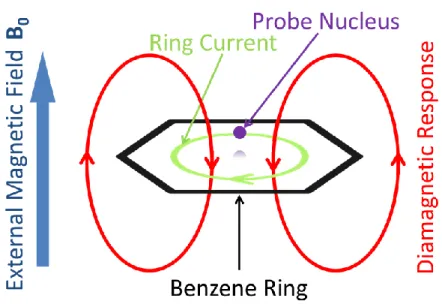
Figure 2.11 Illustration for a benzene molecule and ring current in an external field 𝐵0 ... 40
Figure 2.12 1H NMR magic angle spinning (MAS) spectra of water in P-0 AC with different filling condition: black line represents vapor adsorption, red line represents partial vapor adsorption and injecting water, blue line represents absorption by syringe injection water [109]. ... 41
Figure 2.13 Pore size distribution for different BO PEEK samples ... 42
Figure 3.1 SEM image of dry activated carbon sample of P-90. The scalebar is 500 μm, each subdivision is 50 μm ... 46
Figure 3.2 Specific heat 𝐶𝑃 for water confined in activated carbon P-90, dry activated carbon P-90, and bulk water/ice from temperature 140 K to 300 K under heating rate 10 K/min. Solid black line represents the 𝐶𝑃 for confined water, blue dot line represents 𝐶𝑃 for dry P-90 carbon, red dash dot line represents 𝐶𝑃 of bulk water/ice. All the measurements are under ambient pressure with heating/cooling rate 10 K/min. Green dash dot line is the guideline for experimental supercooled bulk water. [5] ... 48
xvi
activated carbon specific heat. These experiments are running on heating rate 10 K/min. Orange dot line is specific heat of supercooled water in supercool experiment [5] ... 49
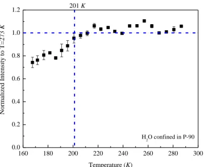
Figure 3.4 Plot of normalized intensity from 1H NMR on water in P-90 AC versus
temperatures ... 51
Figure 3.5 (a) 1H NMR spectra of water confined in P-90 at different temperatures. (b) Plot of full width at half maximum (FWHM) from 1H NMR spectra of water in P-90
versus temperatures. ... 52
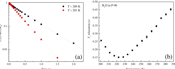
Figure 3.6 (a) Logarithm magnetization versus time at selected temperatures. (b)
Temperature dependence of the 1H NMR spin-lattice relaxation time 𝑇1 for water
confined in P-90 sample... 53
Figure 3.7 Correlation time of water confined in P-90 AC versus temperatures. The red dash dot line is the VFT fitting for the high temperature regime data with 𝑇0 = 176 K and
𝜏0 = 7.4 ps. The activation energy calculated from Arrhenius equation 𝐸𝑎 =
0.207 eV ... 54
Figure 3.8 (a) Temperature dependence of the 1H NMR spin-lattice relaxation time 𝑇1 of mixed water confined in P-90 sample. (b) Correlation time of mixed water in P-90 AC versus temperatures. The red dash dot line is the VFT fitting for the high
temperature regime data with 𝑇0 = 176 K and 𝜏0 = 19 ps. ... 55
Figure 3.9 (a) Temperature dependence of the 1H NMR spin-lattice relaxation time 𝑇1 of
water confined in P-80. (b) Correlation time of water in P-80 versus temperatures. The red dash dot line is the VFT fitting for the high temperature regime data with
𝑇0 = 180 K and 𝜏0 = 3.84 ps. The activation energy got from Arrhenius equation fitting is 0.21 eV. ... 57
Figure 3.10 (a) Temperature dependence of the 1H NMR spin-lattice relaxation time 𝑇1 of water confined in P-94 sample. (b) Correlation time of water in P-94 versus temperatures. The red dash dot line is the VFT fitting for the high temperature
regime data with 𝑇0 = 176 K and 𝜏0 = 2.6 ps. The activation energy 𝐸𝑎 = 0.19 eV ... 58
xvii
Figure 3.12 (a)-(d) 1H NMR spin-spin relaxation time 𝑇2 CPMG measurement for water in P-90 AC at selected temperatures. Y axis is normalized to 𝑀0, black squares are the data obtained from different number of echoes. Red solid lines represent longer 𝑇2
time and blue solid lines represent shorter 𝑇2 time. ... 60
Figure 3.13 (a) 𝑇2 long and short components versus temperatures. (b) Root mean square
distance in long and short 𝑇2 time scale. ... 61
Figure 3.14 (a) The fraction of long and short 𝑇2 component versus temperatures. (b)
Relative population from MD simulation for HDL and LDL local structure versus
temperatures ... 62
Figure 3.15 (a) Derivative of fraction of long and short components in 𝑇2 measurements versus temperature. (b) Mathematical derivative of the fraction of CPMG long 𝑇2
component versus temperatures. The inserted picture is the plot of fraction of CPMG long 𝑇2 component versus temperature and empirical fitting for the fraction plot ... 63
Figure 3.16 Derivative of CPMG long 𝑇2 value of temperature versus temperatures. The red dash dot line is the guideline for reading the data. ... 64
Figure 3.17 (a) Temperature dependence of 1H NMR spin-spin relaxation time 𝑇2 of water in P-80 (b) The fraction of longer 𝑇2 and shorter 𝑇2 components of water in P-80 versus temperatures. (c) Temperature dependence of 1H NMR spin-spin relaxation time 𝑇2
of water in P-94 (d) The fraction of longer 𝑇2 and shorter 𝑇2 components of water in P-94 versus temperatures. Black solid squares represent longer 𝑇2 and red solid dots
represent shorter 𝑇2 ... 65
Figure 4.1 Illustration of volume/enthalpy change for liquid, crystal and glass[124] ... 68
Figure 4.2 (a) Spectra of 1H NMR of water confined in P-90 at different temperatures. (b)-(f) 1H NMR spectra comparison with single pulse measurement and spin-echo pulse measurements of water in P-90 at different temperatures separately. (g) Comparison of spectra at 𝑇 = 177 K for water in P-90 and water in P-0 (h) Full Width at Half Maximum (FWHM) of single pulse 1H NMR spectra of water in P-90 versus
temperatures ... 71
xviii
Figure 4.4 (a) Temperature dependence of the 1H NMR spin-lattice relaxation time 𝑇1 for water in P-90 (b) Correlation time of water in P-90 versus temperatures. The red dash dot line is the VFT fitting for the high temperature regime data with 𝑇0 = 176 K and 𝜏0 = 7.4 ps. The blue dash dot line and green dash dot line is the
guideline for Arrhenius fitting. ... 75
Figure 4.5 (a) Single pulse 1H NMR spectra of water confined in P-80 sample at selected temperatures (b) Single pulse 1H NMR spectra of water confined in P-94 sample at selected temperatures ... 76
Figure 4.6 (a) 𝑇1 relaxation time for water confined in P-80 versus temperatures. ... 77
Figure 5.1 (a) 1H NMR spectrum of water in P-90 at 𝑇 = 168 K. Black solid line is the experimental data. Red dash dot line is the fitted Lorentzian peak, blue dash dot line is the residual of subtraction of experimental data and fitted Lorentzian peak (b) 1H NMR spectra of water in P-90 at selected temperatures. ... 80
Figure 5.2 Spectrum of the hole-burning echo of pure water (open symbols) and of the Hahn echo (solid line) recorded under similar conditions. The oscillations are a Gibbs
ringing artifact. [100] ... 82
Figure 5.3 Hole burning experimental spectra with different parameters. #1 is the single
pulse spectrum at 144 K in highest power ... 83
Figure 5.4 HB spectra for glycol in glass transition process. Three figures from top to bottom represent different pulse length applied on the HB pulse. The ‘narrow’ spectrum used the longest pulse length, and the ‘broad’ spectrum obtained from the shortest pulse length [129] ... 85
Figure 5.5 HB echo for pure water with different D1[130] ... 86
Figure 5.6 (a) Specific heat capacity 𝐶𝑃 of H2O confined in P-90, dry P-90 activated carbon, bulk ice/water. Zoom in the temperature region from 140-190 K from Figure 3.1. (b) Derivative of 𝐶𝑃 with temperature for H2O confined in P-90, dry P-90 activated carbon, and bulk ice/water versus temperatures. (c) Derivative of 𝐶𝑃 in temperature for water confined in P-90 sample at heating rate 10 K/min and 20 K/min versus temperatures, derivative of 𝐶𝑃 in temperature of dry activated carbon and bulk ice with heating rate 10 K/min as reference. (d) Plot of logarithm (𝑄/𝑄𝑠) versus (𝑇𝑔𝑠/𝑇
𝑔)
xix
Figure 5.7 (a) Derivative of 𝐶𝑃 in temperature of water confined in P-80 sample with heating rate 7.5 K/min, 12.5 K/min, 20 K/min. Derivative of 𝐶𝑃 in temperature for bulk ice and dry P-80 activated carbon with heating rate 20 K/min as reference. (b) plot of
logarithm (𝑄/𝑄𝑠) versus (𝑇𝑔𝑠/𝑇𝑔) and fragility calculation for water confined in P-80 ... 90
Figure 5.8 Specific heat 𝐶𝑃 of water confined in different activated carbon samples with
heating rate 10 K/min... 91
Figure 5.9 1H NMR spectra of water confined in different pore sizes at 𝑇 = 144 K ... 92
Figure 6.1 Specific heat capacity 𝐶𝑃 of water confined in P-0 activated carbon, dry graphite, and bulk water/ice from 300 K to 140 K. Red solid line is the 𝐶𝑃 of water confined in P-0, blue dash dot line represents the 𝐶𝑃 of bulk water/ice, and black dot line
represents 𝐶𝑃 of dry P-0 ... 95
Figure 6.2 (a) Normalized intensity of 1H NMR results of water confined in P-0 versus temperatures. (b)1H NMR single pulse spectra of water confined in P-0 at different temperatures ... 96
Figure 6.3 Spectra width of 1H NMR spectra of water confined in P-0. Red dash dot line and blue dash dot line are guideline for data reading ... 97
Figure 6.4 (a) 𝑇1 of water confined in P-0 versus temperatures. (b) Correlation time of water confined in P-0 versus temperatures. (c) 𝑇2 of water confined in P-0 measured by CPMG method versus temperatures. (d) Fraction of long and short component of 𝑇2 for water confined in P-0 versus temperatures. ... 99
Figure 6.5 Comparison of Hahnecho 𝑇2 (short component) and CPMG 𝑇2 (short component) for water confined in P-0 sample ... 101
Figure A.1 1H MAS spectra for water confined in P-90 at T = 289 K and T = 268 K ... 103
Figure A.2 (a) Normalized intensity of water in P-60 versus temperatures. (b) 1H NMR
spectra of water in P-60 at selected temperatures. ... 104
xx
Figure A.4 (a) CPMG 𝑇2 relaxation time for water in P-60 AC versus temperatures. (b) Fraction of long component and short component 𝑇2 for water in P-60 AC versus
temperatures. ... 105
Figure A.5 (a) Normalized intensity of water in P-40 versus temperatures. (b) 1H NMR
spectra of water in P-40 at selected temperatures ... 106
Figure A.6 (a) 𝑇1 relaxation time for water in P-40 AC versus temperatures. (b) correlation time of water confined in P-40 versus temperature. ... 106
Figure A.7 (a) CPMG 𝑇2 relaxation time for water in P-40 AC versus temperatures. (b) Fraction of long component 𝑇2 and short component 𝑇2 for water in P-40 AC versus temperatures. ... 107
Figure A.8 Dynamic crossover temperature versus pore sizes. ... 108
Figure B.1 (a) Experimental 𝑇1 value for bulk water measured. (b) Correlation time
calculated from experimental 𝑇1 of water versus 1000/T. The red dashed line is the best fitting from VFT with fitting parameter 𝑇0 = 176 K ... 109
Figure B.2 Illustration of FID signal from single pulse NMR experiment. The black line is the example of typical FID signal, the red dot line is the signal missing during ring down delay and acquisition delay. ... 111
Figure B.3 1H NMR spectrum for water in P-90 at T = 289 K and fitted spectrum in
Lorentzian shape ... 112
Figure B.4 Linear regression fitting for actual temperature and displayed temperature in temperature range 300 K-210 K. The linear equation from least square fitting is 𝑦 = 1.1504𝑥 − 45.516 with𝑅2 = 0.9996 ... 115
Figure B.5 Linear regression fitting for actual temperature and displayed temperature in temperature range 210 K-180 K. The linear equation from least square fitting is 𝑦 = 0.9467𝑥 − 1.4478 with 𝑅2 = 0.9995 ... 115
xxi
Figure C.2 (a) 1/𝑇1 experimental data plot for different 𝛼 value at T = 287 K. the red dot line is least-square linear regression fitting result. (b) 1/𝑇1 experimental data at different temperatures versus different 𝛼 values. Black dot line is the sketched straight line for reading data. (c) 1/𝑇1 experimental data versus different 𝛼 for water confined in P-90 at T = 228 K. Red dot line is the linear regression fitting for the data. (d) 1/𝑇1
experimental data versus different 𝛼 for water confined in P-90 at T = 177 K. Red
dot line is the linear regression fitting for the data. ... 121
Figure C.3 (a) 1/𝑇1,𝑖𝑛𝑡𝑟𝑎 from Table C.1 versus temperatures. (b) 𝑇1,𝑖𝑛𝑡𝑟𝑎 versus
temperatures. (c)1/ 𝑇1,𝑖𝑛𝑡𝑒𝑟 from Table C.1 versus temperatures. (d) 𝑇1,𝑖𝑛𝑡𝑒𝑟 versus
temperatures ... 123
Figure C.4 (a) Translational diffusion coefficient for water confined in 1.6 nm hydrophilic pores and 2.1 nm hydrophilic pores. (b) Rotational diffusion coefficient for water confined in 1.6 nm hydrophilic pores and 2.1 nm hydrophilic pores. Green dash line is Arrhenius equation fit for the diffusion coefficient at low temperatures. Blue dash line is VFT equation fit for diffusion coefficient at high temperature region. ... 124
Figure C.5 Ratio of rotational and translational coefficient for confined water versus
temperatures. ... 125
Figure C.6 Least-square linear regression fitting weight 𝑅2 versus temperatures. ... 126
xxii
LIST OF ABBREVIATIONS
LDA Low density amorphous
HDA High density amorphous
LDL Low density liquid
HDL High density liquid
LDW Low density water
HDW High density water
LLPT Liquid-liquid phase transition LLCP Liquid-liquid critical point
MD Molecular dynamic
DSC Differential scanning calorimetry
NMR Nuclear magnetic resonance
QENS Quasi-elastic neutron scattering BDS Broadband dielectric spectroscopy
XRD X-ray diffraction
PES Potential energy surface
LSI Local structure index
VFT Vogel-Fulcher-Tammann
RF Radio frequency
CPMG Carr-Purcell-Merbromin-Grannie
HB Hole burning
xxiii
PEEK Polyether ether ketone
MAS Magic angle spinning
1
CHAPTER 1 INTRODUCTION
1.1 Water: The Matrix of Life 1.1.1 Bulk Water
Water is the most abundant and important compound on earth. It covers 71% of the
planet’s surface and I the main constituent of living organisms. As we know, the water molecule
is composed of one oxygen atom and two hydrogen atoms, featuring the O-H bond length of
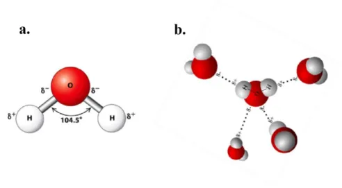
0.9572 Å and a O-H-O bond angle of 104.5° (see Figure 1.1 (a)) [1]. One of the interesting
features of water molecules is their tendency to connect with other water molecules by hydrogen
bonds, ideally forming a tetrahedral structure as shown in Figure 1.1(b). [1]
Figure 1.1 (a) A ball and stick model of a single water molecule. The solid red ball represents the oxygen atom. The solid white balls are hydrogen atoms. (b) A four-coordinated water molecule demonstrating the tetrahedral structure of one water molecule bonding with four other
neighboring water molecules. The hydrogen bond acceptor. The central water molecule accepts two hydrogen bonds from its lower neighboring water molecules and donates two hydrogen bonds to its upper neighbors. [1]
2
The orientation of the hydrogen bonds, variation in hydrogen bond length, and variable
number of coordinated water molecules can affect the local structure of water, resulting in the
anomalous behavior of water [2]. For instance, water may not always be tetrahedral due to
changes in temperature and pressure. This is not the case of most normal liquids, which tend to
have a constant number of coordinates in a wider pressure and temperature range. In general,
when cooling down a liquid to its crystal state, the density will increase due to molecular dense
packing, and therefore the density of crystal is larger than that of the liquid. However, water
experiences the opposite effect. The maximum density of water occurs at 4 °C in the liquid state
than in the ice state. This property is crucial to the ecology system on earth. Because in the cold
winter, rivers, lakes, and oceans, they freeze from the top down, which permit the survival of the
bottom ecology, insulating the water from further freezing, and allowing rapid thawing by
sunlight. Compared to normal liquids, water also has a large specific heat capacity that can be
defined by the fluctuation of entropy (S) as shown in Eq. (1.1) [3],:
< (𝛿𝑆)2 >= 𝑘𝐵𝐶𝑃 (1.1)
in which 𝑘𝐵 is the Boltzmann constant. The high isothermal compressibility, 𝜅𝑇, of water can be
characterized by volume fluctuation as described in Eq. (1.2) [3],:
< (𝛿𝑉)2>= 𝑉𝑘𝐵𝑇𝜅𝑇 (1.2)
The large heat capacity of the seas (4.12 J ∙ g−1∙ K−1) [1] allows them to act as huge heat
reservoirs, such as that sea temperature varies by one-third of as much as the temperature on lan ,
and so moderates the planet’s climate [4]. The low compressibility of water reduces sea level by
3 220 240 260 280 300 320 340 360 380
960 970 980 990 1000 (k g m -3 ) Temperature (K)
277 K
Normal liquids
a.
220 240 260 280 300 320 340 360 380 60 65 70 75 80 85 90 95 100 105 110 CP (J mo l
-1 K -1 )
Temperature (K) 309 K
Normal liquids b.
220 240 260 280 300 320 340 360 380 0.4 0.5 0.6 0.7 0.8 0.9 1.0 1.1 1.2 (GP a -1 ) Temperature (K) 319 K
Normal liquids c.
Figure 1.2 Experimental measurements of the (a) density (ρ) [1], (b) specific heat (𝐶𝑃) [5], and
(c) isothermal compressibility (𝜅𝑇) of bulk water [6] at a temperature range of 380-235 K. The
green dot lines represent the behaviors of normal liquids
The notable properties of water are more accentuated at low temperatures, as shown in
Figure 1.2 (a)-(c). For example, when water is supercooled below its freezing temperature 273 K unlike other supercooled liquids (the green dot lines in Figure 1.2), the specific heat capacity
𝐶𝑃 and compressibility 𝜅𝑇of bulk water increase rapidly toward “infinity” at 235 K. If we fit the
𝐶𝑃and 𝜅𝑇 with a power law function, see Eq. (1.3) (1.4)
𝐶𝑃~ ( 𝑇 𝑇𝑠− 1)
−0.26
(1.3)
𝜅𝑇~ (𝑇 𝑇𝑠− 1)
−0.36
(1.4)
we can find it diverges at 𝑇𝑠 = 228 K from the fitting results [5, 6].
Unfortunately, detailed investigations about supercooled bulk water around 228 K cannot
be carried out experimentally, since bulk water crystallizes rapidly below the homogeneous
nucleation temperature 𝑇𝐻≈ 235 K at atmospheric pressure [7]. So, how to build up a theoretical
model to understand the anomalies of water and how to develop experimental techniques to
capture the supercooled water properties below 𝑇𝐻 become the key to explain the mysteries of
4
1.1.2 Phases of Bulk Water
Phase diagrams show the preferred states of matter at different temperatures and
pressures. With each phase, the material is uniform with respect to its chemical composition and
physical state. The phase diagram of water is complex. For example, ice has 16 known phases at
low temperature and different pressures [8].
Figure 1.3 (a) The state of water at ambient pressure [9]. (b) The temperature-pressure phase diagram of water [10]. The solid black line that divides the orange and yellow-shaded areas at the bottom of the temperature-phase (T-P) diagram indicates a phase transition between LDA and HDA, which has been experimentally observed
Note: 𝑇𝐵 is the boiling temperature, 𝑇𝐵 (𝑃 = 1atm) = 373 K; 𝑇𝑀 is the hexagonal ice (𝐼ℎ) melting temperature, at 1atm, 𝑇𝑀(𝑃 = 1atm) = 273 K; 𝑇𝐻 is the homogeneous nucleation temperature, 𝑇𝐻(𝑃 = 1atm) = 235 K; 𝑇𝑋 is the cubic ice (𝐼𝑐) crystallization temperature, 𝑇𝑋(𝑃 = 1atm) = 150 K; 𝑇𝑔 is the putative glass transition temperature,
𝑇𝑔(𝑃 = 1atm) = 130 K. P represents pressure.
According to Figure 1.3 (a) [9], liquid water can be supercooled to 𝑇𝐻= 235 K, which is
the homogeneous nucleation temperature (𝑇𝐻) and therefore it cannot be cooled further or remain
in the liquid state due to the spontaneous crystallization to hexagonal ice (𝐼ℎ). However, water
can also exist in a glassy state below 130 K by cooling micrometer-sized water droplets at a rate
5
water above 130 K it transforms to a highly viscous liquid that exists up to 153 K [12], at which
point it changes to cubic ice [13]. As marked in Figure 1.3 (a), this temperature range between
153 K to 235 K is called “no man’s land” because there is no stable liquid water survival in this
regime. Therefore, it is extremely difficult to study the nature of the sharp increase of water’s
thermal properties towards 𝑇𝑠 = 228 𝐾 in bulk water by means of experimentation, although
some progress has been recently made [14].
Depending on the pressure (P) and temperature (T), as shown in Figure 1.3(b) , water has
two amorphous states: a low density amorphous (LDA) state, which was first observed by
depositing water vapor on a cold plate 80 years ago [11]; and a high density amorphous (HDA)
state, which researchers discovered by compressing hexagonal ice (𝐼ℎ) below 150 K at high
pressure [15-19].
In addition to the original preparation method based on the vapor and crystalline phases
of water, LDA can be formed directly from HDA, which is called a polyamorphic transition with
a large volume change [20]. The properties of the amorphous states change discontinuously at
this polyamorphic transition [20]. Therefore, the transformation between LDA and HDA appears
to be a first-order phase transition rather than a relaxation phenomenon between two unstable
amorphous changing continuously from LDA to HDA [17].
This well-established first order phase transition between the amorphous states of water
suggests an idea that can be extended to higher temperatures in the “no man’s land” region of the
phase diagram, namely that there exists low density liquid (LDL) and high density liquid (HDL)
whose corresponding glass forms are LDA and HDA [21-24], respectively. The two liquid
H-6
bond and form more tetrahedral structure network, while the HDL is more dense packing and
less tetrahedral structure which interacts with other water molecules by Van de Walls interaction.
The following section will introduce different hypotheses and models that attempt to
explain the anomalous properties of bulk water and the state of supercooled water in the “no
man’s land” region of the phase diagram.
1.1.3 Dissertation Outline
In subsequent chapters, I will discuss the properties of water in a wide temperature range
from room temperature to supercooled region. To access the “no man’s land” temperature
region, we confined bulk water in nanoporous materials by hydrophobic surfaces to avoid
crystallization at low temperatures. DSC and NMR were performed on the nanoconfined water
samples to investigate the structure, thermodynamic, and dynamic properties of water under
nanoconfinement in the wide temperature range.
Chapter 1 briefly reviews the main hypotheses of bulk water in a wide temperature
regime which includes the heterogeneity model of water at high temperature and three models
for supercooled water to explain the anomalies of water properties. The important experimental
evidences, MD simulation results are also reviewed and discussed in this chapter.
Chapter 2 introduces the principle of NMR and DSC techniques, material
characterization methods, and detailed NMR pulse sequence we applied in the experiments.
Chapter 3 reports the structure, thermodynamic, and dynamic properties of water under
hydrophobic nanoconfinement from 290 to 200 K, as measured by NMR and DSC. The
experimental results and simulation discussion show that water has heterogeneity property.
7
crossover is observed at 225 K due to the quick conversion from HDL to LDL which relates to
the intrinsic property of bulk water.
Chapter 4 focuses on the observation of the rotational glass transition of water at 190 K.
At 200 K, LDL dominates the water structure. Below 200 K, there is a second Arrhenius to
Arrhenius transition occurring at 190 K due to change of low-density water molecular tumbling
motion. The NMR spectra analysis shows part of the LDL forms amorphous ice. This is a strong
evidence that supercooled water transfers to the glassy state below 200 K.
Chapter 5 reports another glass transition observed from the endothermic shoulder at 150
K on the DSC curve. We proved only existing “carbon surface/interfacial water/bulk-like water”
sandwich structure would have this transition. So, this glass transition is induced by interfacial
water.
Finally, Chapter 6 I extended my work to the role of interfacial water from 290 K to 140
K. I provided evidence that for monolayer water confined in nanopores, it doesn’t freeze at
extremely low temperature, and have an Arrhenius to Arrhenius transition at 170 K.
1.2 Hypotheses, Simulation Discussions, and Experimental Evidences of Water 1.2.1 Hypotheses of Supercooled Bulk Water
As mentioned in Section 1.1.2, the LDA to HDA first order phase transition and
liquid-gas critical point inspired scientists to have the similar idea to the water in the “no man’s land”.
They assume if heating glassy water to higher temperature, there could have LDL which is the
LDA glass forming liquid and HDL which is the HDA glass forming liquid coexist in “no man’s
land” [26]. For such liquid-liquid coexistence model, there are three main theoretical physics
pictures: (1) stability limit hypothesis [6] (2) singularity-free hypothesis [27, 28] (3) liquid-liquid
8
One of the popular explanations for the anomalous behaviors of liquid water is the
stability limit hypothesis [6], which assumes that the spinodal temperature line, 𝑇𝑆(𝑃), in the
pressure-temperature (P-T) phase diagram of water connects to the locus of the liquid-to-gas
spinodal (i.e., the limit of metastability) of superheated water. It predicts that liquid water cannot
be cooled or stretched beyond the 𝑇𝑆(𝑃) line [29].
Figure 1.4 Illustration of singularity-free hypothesis. The yellow dots represent water connecting each other by non-hydrogen bonds and the blue dots represent water connecting each other by hydrogen bonds
The second theory about supercooled bulk water is called the percolation hypothesis [27,
28, 30-32], which is also referred to as the singularity-free hypothesis (Figure 1.4). It claims that
the thermal response functions of bulk water in the supercooled region have a rapid rise without
singularity. Sastry and Stanley treated bulk water as a network connected with the neighboring
water molecule both by hydrogen bonds and non-hydrogen bonds (Van de Walls interaction).
9
ℋ = ℋ𝑁𝐻𝐵 + ℋ𝐻𝐵 = −𝜖 ∑ 𝑛𝑖𝑛𝑗 <1,2>
𝑖,𝑗
− 𝐽 ∑ 𝑛𝑖𝑛𝑗𝛿𝑖𝑗 <1,2>
𝑖,𝑗
(1.5)
Where the ℋ𝑁𝐻𝐵 is the non-hydrogen bond Hamiltonian and the ℋ𝐻𝐵 represents the
Hamiltonian part for hydrogen bond. 𝜖 and 𝐽 are the energy for non-hydrogen bonds and
hydrogen bonds interaction. 𝑛𝑖, 𝑛𝑗 represent nearest neighbor occupation. 𝛿𝑖𝑗 is the angle
between two nearest water molecules. The heat capacity and other thermal response functions are
solved by the network partition function. This hypothesis considers water as a locally structured
gel comprised of “monomers” (i.e., water molecules) held together by hydrogen bonds and
non-hydrogen bonds. When temperature decreases, the number of monomers held by non-hydrogen bonds
increases. These growing local “patches” formed by water molecules lead to enhanced
fluctuations of specific volume and entropy, which results in a drastic increase of the thermal
response functions of supercooled water, such as specific heat and compressibility. However, the
percolation hypothesis fails to explain the first order phase transition of the amorphous states
from LDA to HDA [27, 33].
The third theory is called the liquid-liquid phase transition (LLPT) hypothesis[26], which
was inspired from the gas-liquid phase transition of water and molecular dynamic (MD)
simulations. As shown in both experiments and theory, below the gas-liquid critical point C (see
Figure 1.5), where the critical temperature 𝑇𝐶 = 647 𝐾 and the critical pressure 𝑃𝐶 = 22 𝑀𝑃𝑎, the superfluid phase separates into two new phases: a low-density gas phase at low pressure and
a high-density liquid phase at high pressure [34]. The thermodynamic response functions are at a
maximum on the Widom line, which corresponds to the maximum fluctuations of structures just
beyond the liquid-gas critical point, C, in the higher temperature and higher pressure region [26].
10
there will also be two phases: a low-density liquid phase at low pressure and a high-density
liquid phase at high pressure [35, 36]. The LLPT hypothesis also predicts there is a Widom line
beyond C’, as the red dashed line shown in Figure 1.5.
Figure 1.5 The liquid-liquid phase transition (LLPT) of water under ambient pressure as predicted by the LLPT hypothesis. C is the liquid-gas critical point and C’ is the hypothesized liquid-liquid critical point around TC’ = 207 K and PC’ = 50 MPa (simulation results) [37]. The
magenta solid line is the coexistence line of HDA-LDA and HDL-LDL predicted from LLPT hypotheses. Dashed red line denotes the Widom line, which intersects with the 1 atm pressure line at 𝑇𝑊= 228 𝐾 [26, 28, 34]
It is of importance to emphasis that the Widom line intersects with 1 atm pressure line at
temperature 𝑇𝑊 = 228 𝐾 [26], which is the same as 𝑇𝑆 (fitted from Eq. 1.3, 1.4).
1.2.2 Hypothesis of Heterogeneity of Water: two-state model
Dating back to 1892, Roentgen’s proposal, he considered water is a mixture of two basic
components, a icelike component and a normal liquid component[38]. Roentgen’s essential idea
has been developed and extended by many researches [39]. This hypothesis has been
successfully in explaining the anomalous properties of bulk water.
Widomline
𝑇𝑊𝑖𝑑𝑜𝑚= 228K
1 atm
𝑇𝐻= 235K
11
Anisimov et. al considered the pure water working as a non-ideal mixed solution[40, 41].
Assume the fraction of state B (LDL) is 𝑥 with chemical potential 𝜇𝐵, and the fraction of state A
(HDL) which has chemical potential 𝜇𝐴 is (1 − 𝑥). The overall Gibbs energy for such mixed
water is Eq. (1.6)
𝐺 = (1 − 𝑥)𝜇𝐴+ 𝑥𝜇𝐵= 𝜇𝐴+ 𝑥(𝜇𝐵− 𝜇𝐴) = 𝜇𝐴+ 𝑥𝜇𝐵𝐴 (1.6)
Where 𝜇𝐵𝐴 is defined as the chemical potential different between state A and B. The
Gibbs energy of the mixture is derived in Eq. (1.7)
𝐺 𝑘𝐵𝑇=
𝜇𝐴 𝑘𝐵𝑇+ 𝑥
𝜇𝐵𝐴
𝑘𝐵𝑇+ 𝑥𝑙𝑛𝑥 + (1 − 𝑥)𝑙𝑛(1 − 𝑥) + 𝜔𝑥(1 − 𝑥) (1.7)
Where 𝜔 is state A and B interaction parameter, variant with temperature and pressure.
However, the two-state model or heterogeneity hypothesis is based on mean field theory
not affected by fluctuation. So, when the fraction 𝑥 approach to the critical fraction 𝑥𝑐, Eq. (1.7)
should consider Landau expansion. The crossover theory developed by Anisimov et. al
[42]combining with the two-state mean field theory in a wide temperature range predicts there is
a sharp change of thermal response function without discontinuity [43].
1.2.3 Liquid-Solid Transition Hypothesis
There is another hypothesis to understand the supercooled water: Chandler thought the
phenomenon predicted in LLPT that stable HDL and LDL phase coexistence at low temperature
high pressure is putative [44]. The liquids demonstrated in LLPT hypothesis are metastable
phases, especially the low-density liquid is suggested to being coarsening of the ordered ice-like
12
Figure 1.6 Pressure-Temperature (P-T) Phase diagram of supercooled water. 𝑇𝑚 and 𝑇𝑠 represent melting temperature and stability limit temperature. Blue region in the P-T plane is the stable state of liquid, red region is where the liquid is metastable, and grey region is where liquid is unstable. The free energy surfaces of liquids are shown above in a function of density and structure orientation parameter 𝑄6. The molecular configurations from simulation are shown below. The white patches are representing liquids, the red patches are coarse grained ice, respectively[45].
Figure 1.6 shows the pressure-temperature phase diagram of bulk water from liquid-solid transition hypothesis. The liquid is the stable equilibrium phase above ice-water melting
temperature 𝑇 > 𝑇𝑚, and is unstable below the stability limit temperature 𝑇𝑠. Between 𝑇𝑠 < 𝑇 <
𝑇𝑚, intermediate region, liquid is metastable phase with respect to crystal ice. In liquid-solid
transition hypothesis, during the intermediate temperature region, the water structure relaxation
is slower when going to lower temperature. When the temperature approach to the stability limit
temperature 𝑇𝑠, coarsening of water occurs on time scale in milliseconds and such water is
preparing to form coarse-grained ice. The free energy surfaces for water below 𝑇𝑠 shows it is not
a stable phase. The snapshot from the simulation box also shows the coarse-grained ice forming
13
In summary, the LLPT hypothesis considers water has a second metastable critical point
at high pressure low temperature. The long-range fluctuation from the critical point could affect
the properties of bulk water at lower pressure higher temperature. The anomalous properties of
water are the influence from the hidden second critical point. The singularity-free scenario
shows, there is the appearance of sharp but continuous changes in density and entropy at low
temperature without hidden critical point. The anomalies of water at ambient pressure
supercooled region can be reproduced by adjusting the water cooperativity parameter. Spinodal
stability limit hypothesis and solid-liquid transition hypothesis both consider supercooled water
is unstable liquid below 𝑇𝑠. The sharp increase of the thermal properties of supercooled water are
due to approaching the stability line. The two-state model is discussing the problem from another
point of view. It treated water as a mixture of two types of clusters. One is liquid-like
(high-density liquid) cluster and the other is ice-like (low-(high-density liquid) cluster. By modulating the
interaction parameter, Anisimov et. al also can reproduce the anomalies of water at ambient
pressure in supercooled regime.
1.2.4 Simulation Results from Different Water Models
Water is a particularly difficult material to simulate because it is a molecular liquid and
researchers have been unable to universally agree on its tractable intermolecular potential [46].
Nevertheless, there is still a distinct advantage of using simulations over experiments when
studying the bulk water. Even the most recent experimental techniques, such as X-ray diffraction
[14] still cannot probe the “no man’s land” region of the phase diagram due to the homogeneous
nucleation of the supercooled water from liquid to ice. However, nucleation will not occur on the
timescale of computer simulations, which is typically in the picosecond range. Therefore,
14
Figure 1.7 Simple water molecule models and their structure parameters. Model types a, b and c are all planar, whereas type d is almost tetrahedral [47]. The middle point site in c and the lone pair sites in d are labeled q2. The model types (a-d) are explained and defined in Table 1.1 Note:𝜎 is the average distance between water molecules; 𝐼1 is the O-H bond length; 𝐼2 is the average distance between oxygen to the nearest neighboring hydrogen; 𝑞1 is the charge on hydrogen; 𝑞2 is the average charge on oxygen; 𝜃0 is the H-O-H bond angle; 𝜙0 is the angle between two nearest neighboring hydrogens
Table 1.0.1 Parameters of Selected Water Molecule Models
Water Model Type 𝝈 (Å)
𝝐 ( 𝒌𝑱
𝒎𝒐𝒍)
𝑰𝟏 (Å) 𝑰𝟐 (Å) 𝒒𝟏 (𝒆) 𝒒𝟐(𝒆) 𝜽∘ 𝝓∘
ST2[48] d 3.1 0.3169 1 0.8 +0.243 -0.2436 109.47 109.47
SPE/C[49] a 3.166 0.650 1 - +0.4238 -0.8476 109.47 -
TIP4P/2005[50] c 3.159 0.7749 0.957 0.1546 +0.5564 -1.1128 104.52 52.26
TIP5P[51] d 3.12 0.6694 0.9572 0.7 +0.241 -0.241 104.52 109.47
15
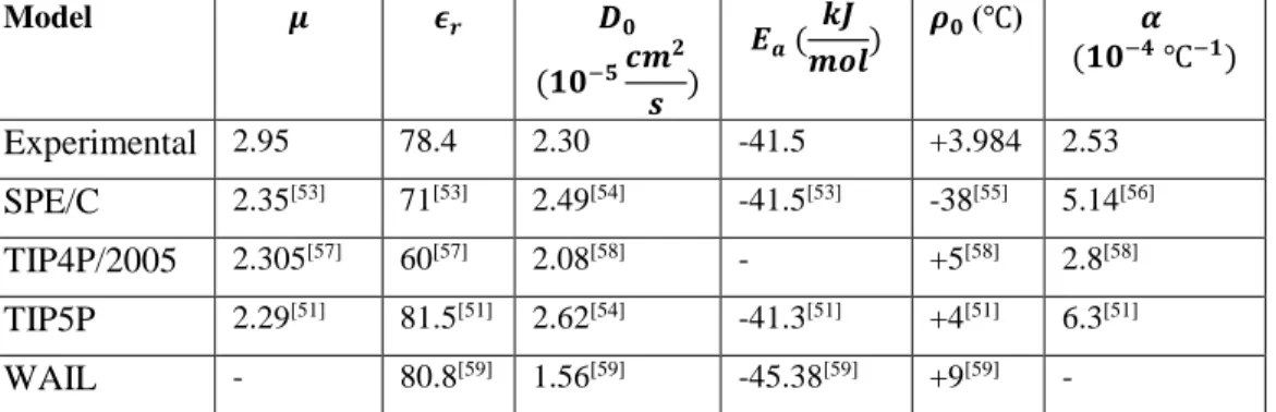
Table 1.0.2 Calculated physical properties of selected water molecule models and experimental data measured from bulk water
Model 𝝁 𝝐𝒓 𝑫𝟎
(𝟏𝟎−𝟓𝒄𝒎
𝟐
𝒔 )
𝑬𝒂 (
𝒌𝑱
𝒎𝒐𝒍)
𝝆𝟎(℃) 𝜶
(𝟏𝟎−𝟒 ℃−𝟏)
Experimental 2.95 78.4 2.30 -41.5 +3.984 2.53
SPE/C 2.35[53] 71[53] 2.49[54] -41.5[53] -38[55] 5.14[56]
TIP4P/2005 2.305[57] 60[57] 2.08[58] - +5[58] 2.8[58]
TIP5P 2.29[51] 81.5[51] 2.62[54] -41.3[51] +4[51] 6.3[51]
WAIL - 80.8[59] 1.56[59] -45.38[59] +9[59] -
Note: 𝜇 is dipole moment; 𝜖𝑟 is dielectric constant; 𝐷0 is self-diffusion coefficient; 𝐸𝑎 is activation energy to break the O-H bond; 𝜌0 is the temperature at maximum density; 𝛼 is thermal expansion coefficient.
ST2 (see Figure 1.7 (d)) water was the first simulated water model developed by
Stillinger et al. in 1974 [48]. It exaggerates the real properties of water when the temperature
approaches 𝑇𝐻 = 235 𝐾. The MD results from the ST2 water model at low temperature and high
pressure support the LLPT hypothesis. However, ST2 overestimates the melting temperature of
ice, 𝑇𝑚, by 30 K [48]. Other water models, such as SPC/E (see Figure 1.7 (a)) TIP5P (see
Figure 1.7 (d)) support the LLPT hypothesis at low temperature also, but SPC/E predicts the maximum density of water is at 240 K [54], and TIP5P predicts the ice 𝐼ℎ state to be metastable
[51]. TIP4P/2005 (see Figure 1.7 (d)) is widely used nowadays. It predicts the maximum density
temperature at 278 K. Figure 1.8 shows the snapshot of simulation results for TIP4/2005 water at
room temperature and supercooled region. It is clear to see that water has two different local
structures: HDL (yellow patches) and LDL (blue patches). At room temperature, water structure
is dominated by HDL (less tetrahedral) structure. While at supercooled region, water structure is
dominated by LDL (more tetrahedral) structure. Nilsson et. al have observed the continuous
conversion between HDL to LDL by lowering temperature at ambient pressure. He concludes
16
hypothesis. But TIP4/2005 doesn’t predict the melting temperature for ice-water transition
precisely, it gives a 𝑇𝑚 that is 20 K lower [58, 60]. There are also other models, such as the mW
model, do not support LLPT, but rather suggest micro-crystallization of supercooled water
occurs [45, 61]. However, none of these models were able to predict the phase diagram around
the ice (𝐼ℎ) melting temperature.
17
hypothetical LLPT phase diagram. The yellow patches represent HDL water and blue patches represent LDL [62]
Figure 1.9 (a) The relative population of high-LSI and low-LSI from TIP4/2005 simulation results versus temperatures [63] (b) Hypothetical temperature dependent heterogeneity of water. The density of water separated in normal region and anomalous region. The blue solid line is the simulation result, the inserted pictures illustrate the continuous transition from HDL to LDL. From right to left, HDL dominated water structure, fluctuation into dense packing HDL liquid, HDL patches into LDL liquid, LDL dominates liquid. [62, 64]
Figure 1.9 (a) plots the conversion between local HDL and LDL versus temperature, (b) shows such local structure conversion resulting the anomalies of water. The local structure
continuous conversion gives the anomalies of water at ambient pressure.
Recently, a new model named WAIL derived from Adaptive Force Matching for Ice was
created through quantum and molecular mechanics calculations by fitting a coupled-cluster
quality potential energy surface (PES) of water [52, 65]. The WAIL water predicts the 𝑇𝑚 of ice
(𝐼ℎ) to be 270 K [59] and the temperature at its maximum density at 282 K [59].
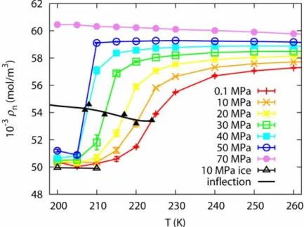
The LLPT in supercooled water was observed by applying the WAIL model (Figure
18
linear response as a function of temperature. The simulated liquid-liquid critical point occurs at a
pressure and temperature of 50 MPa and 207 K [37].
Figure 1.10 Density isobars of supercooled water from 200–260 K and 0.1–70 MPa. The densities of WAIL ice (𝐼ℎ) at 10 MPa from 200–210 K is plotted as reference. [37]
In summary, the WAIL model describes the properties of water most accurately among
these tremendous water models.
For this dissertation, we collaborated with Professor Limei Xu’s group in Peking
University who has expertise in WAIL water model simulations so that we could get the
information of the diffusion coefficient of confined water and the local structures of supercooled
water. Determining the rotational and translational diffusion coefficients will help us to
understand the dynamic properties of water (e.g., molecular motions). Additionally, investigating
the local structures of water may enable us to determine the existence of possible molecular
structures in supercooled water. However, due to the limitations of the simplified energy, there is
19
important in MD simulation, therefore in order to confirm or disprove the theory and
simulations, it is still necessary to collect experimental data.
1.2.5 Nanoconfined Water Experiments
Decades ago, scientists found when they confined water in nanopores, such as MCM-41
(a porous hydrophilic silica nanotube) [66-77], SBA-15 (a micellar material) [78], and layered
vermiculite clay [79, 80], the freezing point could be suppressed to a low temperature region [81,
82], even avoiding crystallization altogether [82].
Figure 1.11 The heat capacity (𝐶𝑃) of water confined in MCM-41 featuring different pore sizes (1.5–2.1 nm). The dashed line is the 𝐶𝑃 of bulk water and ice, provided for reference [83]
Recent experimental studies on water confined in MCM-41 shed light on ways to
investigate the properties of supercooled water in the “no man’s land” region of the phase
diagram. The specific heat capacity of water confined in different MCM-41 pore sizes showed
that in a system featuring 2 nm-sized confinement or less, there was no fusion of ice (Figure
20
Figure 1.12 (a) The inverse of the diffusion coefficient versus 1000/T as measured by NMR for water confined in 1.4 nm MCM-41. (b) Translational correlation time of water confined in MCM-41 samples in 1.4 nm pores versus 1000/T as measured by QENS [69, 84].
Quasielastic neutron scattering (QENS) and nuclear magnetic resonance (NMR)
spectroscopy are two techniques that can be used to probe the dynamics of a material. Figure
1.12 (b) demonstrates the correlation time of water molecules obtained from QENS experiments on water confined in an MCM-41 samples. In this plot, there is a dynamic crossover temperature
𝑇𝐿 at 225 𝐾, which was found from the intersection of two different types of correlation time
fittings (Vogel-Fulcher-Tammann (VFT) fitting and the Arrhenius fitting, which will be further
MCM-21
41measured from pulse gradient NMR also showed a similar transition temperature at 223 ± 2 𝐾
(see Figure 1.12 (a)). The Chen’s group considered such a dynamic transition as related to the
second critical point in LLPT theory. 225 K is the temperature where the fluctuation of the two
liquids (VFT and Arrhenius) reaches a maximum by the definition of Widom line [69, 84].
However, the claim remains in question. Vogel’s group shows for water confined in
MCM-41, it has step crystallization below 250 K, the observed transition and other dynamic
changes may be induced by micro-crystallization. These experiments and active discussions
bring up following questions in our research:
(1) Is the water homogeneous or heterogeneous naturally?
(2) Is the LDL existing at low temperature region if water is not freezing?
(3) Is the dynamic crossover induced by micro-crystallization instead of LLPT?
(4) How does the surface effect or nanoconfinement effect affect the properties of water?
(5) What is the mechanism for water’s glass transition?
My main focus in this dissertation is trying to understand the physics behind the
anomalous behavior of water. To access the “no man’s land”, we applied water confined in
hydrophobic surfaces. To investigate the properties of confined water, we performed DSC and
NMR methods to study the thermodynamic and dynamic properties of water.
In our experiment, most importantly, we captured the macroscopic heterogeneity of water
at room temperature and proved LDL is a stable liquid state at low temperature. We also noticed,
above 200 K, there is no crystallization for supercooled confined water and has a dynamic
crossover temperature at around 225 K which is the same as water confined in hydrophilic pores.
This is a strong evidence to prove the dynamic crossover is not induced by micro-crystallization
22
glass transition of water and a growth of amorphous ice. Finally, we found there is a glass
23
CHAPTER 2 EXPERIMENT METHOD, SAMPLE PREPARATION AND CHARACTERIZATION
2.1 Nuclear Magnetic Resonance (NMR)
Studying the structure and dynamics of a material is generally performed using X-ray
diffraction (XRD) [25, 87, 88], rheology, or various optical methods [89, 90]. However, these
techniques can only measure bulk material properties. For confined systems, X-ray fails to
penetrate the surface. shear stress cannot be applied on the material in the pores, optical methods
only give local structure information. In contrast, NMR is uniquely suited for probing local
structures and dynamic properties of liquids or gases inside porous media, as long as it contains
nuclear spin [91].
In this dissertation, we applied NMR to probe the size distribution of activated carbon
micropores (< 2 nm), as well as to investigate the state of water confined in the nanopores,
including the dynamics and local structure [92]. Therefore, it is necessary to review some of the
basic concepts of NMR prior to its application in this research.
2.1.1 Magnetization
Materials are made of atoms. Atoms have electrons and nuclei. Every nucleus has mass,
electric charge, magnetism, and spin. The magnetism of a nucleus can interact with a magnetic
field. The spin of nucleus acts like it is spinning around, rotating in space like a planet. Nuclear
magnetism and nuclear spin are sensitive to the molecular environment, for example, the
24
with an excellent tool for spying on the microscopic and internal structure of objects without
destructivity.
Table 2.1 Gyromagnetic ratio of the nuclei used in NMR spectroscopy [93]
Nucleus Spin Natural Abundance (%) 𝜸 (𝟏𝟎𝟔 𝒓𝒂𝒅 ∙ 𝒔−𝟏∙ 𝑻−𝟏) 𝜸
𝟐𝝅 (𝑴𝑯𝒛 ∙ 𝑻
−𝟏)
1H 1/2 99.9885 267.513 42.576
2H 1 0.015 41.066 6.539
13C 1/2 1.07 67.262 10.705
19F 1/2 100 251.662 40.053
Note: 𝛾 is gyromagnetic ratio
A rotating object possesses a quantity called angular momentum. In quantum mechanics,
angular momentum is quantized as 𝐼ℏ, in which 𝐼 is the spin quantum number and ℏ is Planck’s
constant. The dipolar magnetic momentum can be defined as 𝜇 = 𝛾𝐼ℏ, where 𝛾 is the
gyromagnetic ratio. When an external magnetic field (𝐵0) is applied to a nuclear state with spin
𝐼, it will degenerate to (2𝐼 + 1) sublevels featuring magnetic quantum numbers (𝑚) of −𝐼, −𝐼 +
1, … 𝐼 − 1, 𝐼. Table 2.1 lists the spin number and gyromagnetic ratio for selected nuclei. For
example, 1H has a nucleus of spin ½. When 𝐵0 is applied, the equilibrium energy state will split into two different energy states, featuring an energy (𝐸𝑚) of 𝜇𝐵0 = −𝛾𝐼ℏ𝐵0 = −𝑚𝛾ℏ𝐵0 =
±1
2𝛾ℏ𝐵0 (see Figure 2.1). The spins will possess along the external field axis with the Larmor
25
Figure 2.1 Illustration of a 1H nucleus in an external magnetic field [93]
In thermal equilibrium, the probability for a spin to remain at the split energies follows
the Boltzmann distribution 𝑃𝑚 ∝ exp(−𝐸𝑎/𝑘𝐵𝑇), in which 𝐸𝑎 is the degeneracy energy and 𝑘𝐵
is the Boltzmann constant. The net magnetization, M0,for N non-interacting spins follows Eq.
(2.1):
𝑀
0= 𝑁𝛾ℏ
∑ 𝑚𝑒𝑥𝑝(𝑚𝛾ℏ𝐵0
𝑘𝐵𝑇 )
𝐼 𝑚=−𝐼
∑ exp(𝑚𝛾ℏ𝐵0
𝑘𝐵𝑇 )
𝐼 𝑚=−𝐼
. (2.1)
At the high temperature limit, 𝛾ℏ𝐵0 ≪ 𝑘𝐵𝑇, Eq. (2.1) can be simplified to:
![Figure 1.3 (a) The state of water at ambient pressure [9]. (b) The temperature-pressure phase diagram of water [10]](https://thumb-us.123doks.com/thumbv2/123dok_us/8280509.2192895/27.918.247.670.314.659/figure-state-water-ambient-pressure-temperature-pressure-diagram.webp)