Continuum direction vectors in high dimensional low sample size data

(1)

Continuum Direction Vectors in High Dimensional Low Sample

Size Data

Myung Hee Lee

A dissertation submitted to the faculty of the University of North Carolina at Chapel Hill in partial fulfillment of the requirements for the degree of Doctor of Philosophy in the Department of Statistics and Operations Research (Statistics).

Chapel Hill 2007

Approved by

Advisor: Dr. J. S. Marron

Reader: Dr. Yufeng Liu

Reader: Dr. Andrew Nobel

Reader: Dr. Ivan Rusyn

Reader: Dr. Haipeng Shen

(2)

(3)

ABSTRACT

MYUNG HEE LEE: Continuum Direction Vectors in High Dimensional Low Sample Size Data

(Under the direction of Dr. J. S. Marron)

(4)

ACKNOWLEDGMENTS

I would like to express my deepest gratitude to my advisor, Professor Steve Marron for his guidance and support. I am very grateful for all the effort that he has made for me, especially over the past two years when he has gone through challenging times in his life. I am privileged to be his student.

I would like to deliver thanks to other committee members, Andrew Nobel, Yufeng Liu, Haipeng Shen, David Threadgill, and Ivan Rusyn for their valuable suggestions on this dissertation. Especially, I would like to thank Ivan Rusyn for kindly providing the data which led to an interesting application.

(5)

LIST OF FIGURES

2.1 Illustrates that the OLS fit XβˆOLS _{is the projection of} _Y _{onto the}

space M={Xβ|β ∈_Rd_{} ⊆}

Rn. . . 8 2.2 Depicts the construction of the PC direction vector. The first direction

accounts for most variation of the data and the second direction is orthogonal to the first. . . 18 2.3 Toy Example with 2−dimensional regression data (xi1, xi2, yi)}501 . A

snapshot from the movie, Lee (2005c). Left: A subspace, represented by the cyan plane, is generated by the arbitrarily chosen direction vector, v, and the output variable,Y. Each data point- blue cross- and its projection on this plane- red circle- are linked together by red lines.

Right: The blue plane pulled from the left side. The red dots form the data for the 1-dimensional regression analysis using the transformed variable,v0X as a regressor. . . 20 2.4 Toy Example with the same 2−dimensional regression data (xi1, xi2, yi)}501

as in Figures 2.2 and 2.3. (a) Projection of input data onto the first PC direction vector in the (X1, X2) plane (b) Scatter plot of the first

PC against output data (c) Projection of input data onto the second PC direction vector (d) Scatter plot of the second PC against output data, showing that it is the second PC that carries the important in-formation about the output data (i.e., much stronger correlation with

Y). . . 22 2.5 Toy Example with the same 2−dimensional regression data{(xi1, xi2, yi)}501

as in Section 2.3.3. The cyan plane stands for the X-space. The first direction vectors for OLS, PLS, and PCR are drawn. The OLS direc-tion is nearly orthogonal to the PCR direcdirec-tion, and the PLS direcdirec-tion lies between the OLS and the PCR directions. . . 23 2.6 Toy Example with the same 2−dimensional regression data (xi1, xi2, yi)}501

(8)

2.7 Heat map view of Gene Expression from 36 mouse samples. Columns represent genes (variables) and rows display gene profiles from samples (observation). Note that transposing this map is the usual way of displaying. We take this view because the mouse strain labels on the right are clearly labeled. . . 28 2.8 PCA Scatter plot of Gene Expression data. Colors and symbols

indi-cate strains and treatments, respectively. Diagonals are 1-dimensional projections on the first 4 PC directions and off-diagonals are 2- dimen-sional projections on the subspaces generated by those directions. . . 30 2.9 The bar graph of the output data, Blood Alcohol Concentration. Mouse

samples (x-axis) are grouped as strain (A/J, ..., C57BL/6J) and within a strain, alcohol-treated(T)/ control (C) samples are grouped together. We see an obvious effect by alcohol treatment and some variability be-tween mouse strains. . . 31 2.10 Rank tracking plot of the top 100 ranked genes from OLS (α = 0).

Most genes stay highly ranked until α goes to 0.5 (PLS). Afterwards, a portion of genes disappear (low ranked) as we get closer to PCR and none of the genes survive at the very end,α= 1 (PCR). . . 32 2.11 Rank tracking plot of the bottom 100 ranked genes from OLS (α= 0).

About half of genes appear to be highly ranked until α reaches 0.9 and all genes but 3 genes suddenly disappear when α = 1. Genes responsible for the PC direction, which explains the most variability in the samples, could be very different from the genes relevant to the response variable (α = 0). . . 33 2.12 loading tracking plot for 5 direction vectors- the 2nd PC, PLS, OLS,

DWD, MD. Each gene is represented by a piecewise line, connecting the entries of the respective directions. A few genes stand out as important across all the methods. . . 35 2.13 loading tracking plot, with several genes of interest highlighted. The

50 top genes based on the absolute value of OLS are colored as red, 50 based on DWD colored as blue, and purple for genes selected by both. 36 2.14 Scatter plot of OLS and DWD gene loadings. Genes are distributed

(9)

3.1 Two paired sets of 2-d data vectors and the projections of the two direction vectors are shown in the left panels. The scatter plot of data projections are seen in the right panel. This show a weak correlation between the paired projections. . . 44 3.2 Two paired sets of 2-d data vectors and the projections of the CCA

direction vectors are shown in the left panels. The scatter plot of data projections onto CCA vectors are seen in the right panel, which clearly shows a strong correlation. . . 45 3.3 For the same two sets of 2-d data vectors as in Figure 3.1 and 3.2,

shown in the left are the CCA direction vectors, and in the right PCA direction vectors. The two vectors are almost perpendicular, in both the X and Y spaces, showing CCA can be very different from PCA. . 49 4.1 Quantile-Quantile Envelope plot for testing the distribution of {bλ1

λ1}

against theχ2

n−1/n distribution. The red curve is inside the blue

bun-dle, which shows the validity of the asymptotics. . . 77 4.2 Quantile-Quantile plot for testing distributional form of {d (u1ub1)

2_}

against the χ2 _{distribution.} _{The red curve shows the quantiles of}

{d (u1ub1)

2_{}, and the green line indicates the theoretical quantiles from}

the χ2

n−1 distribution. The blue curves show the variation of quantiles

existing in aχ2

n−1 random sample. The red curve is inside the bundle

(10)

CHAPTER 1

Introduction

Data with more variables than observations are emerging in a number of fields. For example, in typical microarray experiments, expression level of numbers of genes ranging from the thousands to the tens of thousands are measured, while the number of observations (i.e., tissue samples) is typically a few tens or hundreds. Data from text recognition and signal processing also often have a much larger dimensiondthan sample size n. The term High Dimensional Low Sample Size (HDLSS) will be used to refer to this type of data in this dissertation. Another term in use for this type of setting are “large p, small n” .

The statistical analysis of HDLSS data has become a serious challenge to statisti-cians over a number of years. Classical multivariate tools, originally developed under the assumption of d < n, seldom provide satisfying results for HDLSS data. One of the main reasons for this failure is because there is not enough information (ob-servations) to estimate the full underlying covariance matrix. An important step in multivariate analysis is to sphere the data by pre-multiplying the root inverse of the covariance matrix. The fact that the estimated covariance matrices from HDLSS data are inevitably singular hinders this key step in practice.

(11)

introduction and overview), the LASSO (Tibshirani, 1996), and the elastic net (Zou and Hastie, 2005) can be viewed as modified Ordinary Least Squares (OLS) methods, which can be applied to HDLSS input data. The Support Vector Machine (SVM) (see e.g. Vapnik (1982); Vapnik (1995); Shawe-Taylor and Cristianini (2000)) is a clever and powerful discrimination method. Marronet al.(2007) developed Distance Weighted Discrimination (DWD), which can be seen as an improved version of the SVM which has good performance with HDLSS data.

Among many attempts to analyze HDLSS data, dimension reduction techniques, based on some directions of interest, are mainly considered in this dissertation. For example, Principal Component Analysis (PCA) finds a set of direction vectors for explaining most of the variability in the data. These direction vectors can be used in several ways. One application is directions for visualization. One can produce 1-dimensional projection plots on those directions or low 1-dimensional projection plots on the subspaces generated by those direction vectors. Another application is to find important variables by sorting on the components of the direction vectors.

HDLSS data also motivate a new type of mathematical theory. Along with the development of new methodologies has come a new family of asymptotics, with the dimensiondincreasing. More detailed discussion on this topic, along with a literature review, can be found in Chapter 4.

In Chapter 2, Continuum Regression (CR) (Stone and Brooks, 1990) will be viewed as a family of direction searching methods, which includes three popular methods, Ordinary Least Squares (OLS), Partial Least Squares (PLS) and Principal Compo-nent Analysis (PCA) as special cases. Each of these will be studied in the HDLSS setting. The novel HDLSS use of this methodology is illustrated by an application to microarray experiments. The change in the relative gene weights, implied by these different directions, will be studied.

(12)

multi-variate data sets are obtained in pairs, Canonical Correlation Analysis (CCA) provides a simple method for understanding the connection between the two data sets. PLS and PCA are also generalizable in this scenario. All of these methods will be under-stood as simultaneous direction searching methods over two high dimensional spaces. As a generalization of CR for paired HDLSS data settings, we propose Continuum Canonical Correlation (CCC), which includes the above as special cases.

(13)

CHAPTER 2

Continuum Regression

Suppose we have a set of data which consists ofnpairs (xi, yi) fori= 1,· · · , n.Let

xi ∈ Rd represent a regressor vector (i.e., input, i.e., covariates) and yi ∈ R denote

the response (output) value from the i-th observation. In the regression problem, the goal is to explain or predict the quantitative response variable Y as a function

f(X) of the d-dimensional regressor vectorX = (X1,· · · , Xd)0 based on the training

data {(xi, yi)}ni=1. The linear model assumes that the regression function, or the

conditional expectation of E(Y|X) = f(X) has the form f(X) = β0 +Pd_j₌₁Xjβj.

Despite the limitation of model structure, the linear model

(i) is simple and gives an interpretable description,

(ii) has been studied for a long time, so the resulting algorithms are efficient and well understood, and

(iii) can be generalized into non-linear regression via transformation of the regressor variables.

In the example that we have in mind, the response variableY is a phenotypic mea-surement assumed to be quantitative. The regressor variables (X1,· · · , Xd) are gene

(14)

As a result, in microarray studies, the number of variables, d, oftentimes, is much larger than the number of samples, n. This type of data will be refereed to as High Dimensional Low Sample Size (HDLSS) data in this dissertation.

Probably the most simple way to fit a linear regression function is the Ordinary Least Squares (OLS) method. However, the OLS method directly applied to HDLSS data usually does not provide satisfactory results. See Section 2.2 for details. When the input variables dexceeds the number of data points n, among many alternatives to the OLS method, two commonly considered approaches are the shrinkage method and the method of linear transformation. The former includes ridge regression (see Hoerl and Kennard (1970); Hastieet al. (2001) for useful introduction and overview), the LASSO (Tibshirani, 1996), and the elastic net (Zou and Hastie, 2005). All these methods impose a penalty on the regression coefficient size (in L1, L2, or in both

senses) and these constraints make the solution coefficients shrink.

We focus on linear transformation methods in this dissertation; a detailed ex-planation can be found in Section 2.3. Special examples include Principal Compo-nent Regression (PCR) and Partial Least Squares (PLS). These methods sequentially produce linear transformations (i.e., direction vectors) of the input variables, and use a small number of the direction vectors as regressors. Continuum Regression (CR), proposed by Stone and Brooks (1990), brings OLS, PLS and PCR under one mathematical umbrella. Including these three methods as special cases, they formu-lated a richer family of regression procedures by introducing a continuous parameter

α∈[0,1], which controls the tradeoff between the covariance (between the input and the output data) and the variance (of the input data). In particular, for α = 0,1/2,

(15)

In this dissertation, however, CR will be applied to microarray data in a slightly differently sense than its original purpose (i.e., predictive modeling). CR will be viewed as a family of direction searching methods. As opposed to the original CR or shrinkage regression methods mentioned in the paragraphs above, choice of a single “best” tuning parameter is not our goal. Rather, we study the entire family of direction vectors over the whole range of the continuum parameter because each of these illustrates a different aspect of the data. This point is reflected in the term “continuum direction vectors” in the title of this dissertation. See Section 2.4 for details.

In this chapter, we will first review CR and its special cases in the original context, i.e., from the regression point of view. We begin the chapter by introducing notation in Section 2.1 and review the OLS and study its behavior in HDLSS settings in the following section. In Section 2.3, we establish a general framework for dimension reduction and will discuss PCR, PLS, and CR, with examples as special cases of this framework. Finally, in Section 2.4, an application of CR to microarray data will be discussed.

2.1 Notation and Assumptions

We denote the regressor (input) variables by X = (X1,· · · , Xd)0 and a scalar

response (output) variable by Y. The data,n samples of those variables, are written in lower case lettersxi ∈Rdand yi ∈Rfori= 1,· · · , n. Bold upper case letters refer

to data matrices; we write input and output data matrices as

X=      

x0₁

.. .

x0_n

     

n×d

and Y =

      y1 .. . yn      

(16)

Note that the i-th input data is denoted by a column vector xi, but is stored as a

row vector x0_i in the data matrix X to be consistent with the typical way of writing the data matrix in the linear regression literature.

Column vectors with n components are written in bold lower case, for example, the j-th column ofX is denoted byxj forj = 1,· · · , d. It containsn observations on

the j-th regressor variable,Xj. This convention distinguishes the data vector on the

j-th variable xj ∈Rn from the input data from the i-th sample xi ∈Rd.

We assume that the columns of X (variables) and Y have been centered to have sample mean zero; i.e., each element of the data matrices, xij and yj, have been

replaced by xij − _n1Pn_i0₌₁xi0_j and y_i − 1

n Pn

i0₌₁yi0, respectively. Thus, the sample covariance matrix Cov(X)d×d and Cov(X, Y)d×1 (multiplied byn−1) will be denoted

as

S =X0X and s=X0Y. (2.1)

Linear regression techniques will be applied to the centered data as the result can always be transformed back to the original data later.

2.2 Ordinary Least Squares

The linear model assumes that the regression function has the form f(X) =

Pd

j=1Xjβj. There are many ways to estimate the regression coefficients, βj, and by

far the Ordinary Least Squares (OLS) method is the most common and convenient way. The OLS estimates ˆβj, j = 1,· · · , d are chosen to minimize the residual sum of

squares over the data,

RSS(β) =

n X

i=1

(yi− d X

j=1

xijβj)2.

We can write this in a matrix notation,

(17)

where β = (β1, β2,· · · , βd). Differentiating with respect to β and setting it to be 0,

we obtain the normal equations

X0Y−X0Xβ = 0. (2.2)

If the inverse of X0X exists, then the OLS estimates are uniquely given as ˆβOLS ₌

(X0X)−1_X0_{Y. The fitted values at the input training data are}

ˆ

Y = XβˆOLS

= X(X0X)−1_X0_Y

and at an arbitrary pointx0 = (x01,· · · , x0d)0, we use the OLS predictors

ˆ

Y =x0₀βˆOLS (2.3)

as a predicted value.

2.2.1 Geometry in

_R

n

The geometry of _Rn _{is helpful to understand how the OLS works with} _n _training

data, and it is illustrated in Figure 2.1. Y ∈_Rn _{denotes the output data vector and}

Xβ =x1β1+· · ·+xdβd∈Rn is a linear combination of column vectors of X. Recall

that xj ∈ Rn is the data vector for the j-th input variable. Let M, represented by

the cyan plane in Figure 2.1, be a closed subspace of _Rn that is generated by the

n-dimensional data vectors for d input variables, namely,

M ={x1β1+· · ·+xdβd|βj ∈R, j = 1,· · · , d}

={Xβ|β ∈_Rd_}_.

(2.4)

(18)

Figure 2.1: Illustrates that the OLS fit XβˆOLS _{is the projection of} _Y _{onto the space}

M={Xβ|β ∈_Rd_{} ⊆}

Rn.

The classical projection theorem tells that there is a unique element Xβˆ ∈ M closest to Y and it is obtained by making the residual vector Y −Xβˆ orthogonal to M. The unique element Xβˆ is called the projection of Y onto M. The normal equation (2.2) ensures that the least squares fitXβˆOLS is indeed the projection ofY onto M, Xβˆ, since

Y−Xβˆ is orthogonal toM.

⇐⇒x0_j(Y−Xβˆ) = 0 j = 1,· · · , d.

⇐⇒x0_jY =x_j0Xβˆ j = 1,· · · , d.

(19)

2.2.2 Motivation for dimension reduction

It might happen that the dimension of the subspace, M, is less than d, i.e. X is not of full column rank because

regressors have an exact linear dependence (e.g. x1 = 2x2), or

the number of variables, d, exceeds the number of observations, n.

For both cases, any element in M, say Xβ, can have a different representation Xβ∗, where β∗ 6=β. Referring to the geometry of _Rn_{, the projection of} _Y _onto _{M, ˆ}_{Y, is}

still unique, we just have more than one expression for it in terms of Xβ. The OLS method for these type of data is not satisfactory for predicting the Y value for a new inputx0 since the choice of the OLS solutionsβ will give an arbitrary predictionx00β.

When there is only an approximate linear dependence among regressors, X0X could be nearly singular. The OLS solution to the normal equation (2.2) is unique, but it could be very unstable, resulting in the estimated coefficients having large variance, hence, poor prediction accuracy.

The first case, including the case when regressors have an approximate linear dependence, has been a motivation for dimension reduction in the classical statistics literature. For these data redundancies, it can be helpful to consider a reduced set of regressors. With a subset selection approach, we could select a subset of regressors according to a certain rule, for example, forward or backward selection procedures. Assume for now that the rows of the data matrix are “ordered” in a way that the “reduced” model can be written in the form

f(X) =

ω X

i=1

Xiβi (2.5)

(20)

the model is rich enough to explain important underlying phenomena.

The data dimension reduction schemes which we will study in this dissertation are motivated by the second case. Keeping in mind the applicability of the regression techniques to microarray data, it is likely that many genes are working together for regulating a specific phenotype. If prediction is the only concern, we could reduce dimension by dropping some genes from the model just like (2.5), and improve the prediction accuracy. This approach has the potential risk of discarding important genes from the model. It can be very important to biologists not to miss genes which play important roles. The way we reduce the data dimensionality should be different from (2.5) in this case, and we defer the detailed review of this issue to Section 2.3.

2.2.3 The choice of OLS solution for HDLSS case

As we saw in the previous section, the OLS solution for HDLSS is not uniquely determined. In some situations, however, we might want to choose an OLS estimate to make a comparison with other methods. When we do not have enough information to specify a solution, an approach to resolve this is to restrict or bias the solution in some way. Two ways of resolving this are discussed in the following sections.

Restriction of the subspace

If we restrict the OLS solution, β, to be in the subspace, U ⊆ _Rd _{generated by}

the d- vectors of training inputs, i.e.,

U ={Pn_i₌₁xiαi|αi ∈R, i= 1,· · · , n}

={X0_α_|_α_{= (}_α

1,· · · , αn)0 ∈Rn},

then we now projectY onto the subspaceM∗ ₌_{X_β_|_β _{∈ U } ⊆ M}₌_{X_β_|_β _∈

Rd}. Thus, the least squares problem becomes

arg min

α∈Rn

(21)

Assuming that XX0 is invertible, the solution is given as ˆα = (XX0)−1_Y. _Call

ˆ

βdual ₌_X0_α_ˆ ₌_X0_(XX0₎−1_Y_.

Ridge solution and its dual solution

The Ridge Regression solution ˆβRidge_{= (X}0_X₊_λ_I)−1_X0_Y _{was proposed by Hoerl}

and Kennard (1970) as a remedy to instability of the OLS solution when X0X is singular or nearly singular. The ˆβRidge _{solves a modified least squares problem,}

ˆ

βRidge=argminβ(Y−Xβ)0(Y−Xβ) +λ||β||2

where λ > 0, called the ridge parameter, controls the balance between the residual sum of squares and the squared length of the parameter vectorβ; the ridge regression solution isshrinked toward 0 in the sense that, theλlarger, the length ofβ is smaller. When λ = 0, we get back to the OLS problem. A dual version of the ridge solution, (Shawe-Taylor and Cristianini (2004) and Saunders et al.(1998)), namely, as a form of ˆβRidge ₌_X0_α ₌Pn

i=1xiαi for some α ∈R

n_{, is obtained with} _α_{= (XX}0₊_λ_I)−1_Y

forλ _>0.The OLS dual solution corresponds to the special case of ridge dual solution with the choice ofλ = 0. From now on, we let ˆβOLS ₌_X0_(XX0₎−1_Y_.

2.3 Dimension Reduction

In this section, a general approach (Stone and Brooks, 1990) to reduction of the dimensionality for HDLSS data, is introduced. The idea behind this approach is that if we can summarize data set of high dimensional covariates,X= (X1,· · · , Xd)0,

into linearly independent factors,Z = (Z1,· · · , Zω)0, whereZm =v0mX, a linear

transformation of the covariates for some vm ∈ Rd, (e.g. vm could be PCR or

PLS direction), for m= 1,· · · , ωd,

(22)

This framework contains Principal Component Regression (PCR), Partial Least Squares (PLS), and Continuum Regression (CR) as special cases.

2.3.1 Linear Transformation of the Input Data

Motivated by thinking of (2.5), we now consider a reduced regression model

f(Z) =

ω X

m=1

Zmθm, (2.6)

where Zm = v0mX, is a linearly transformed variable for vm ∈ Rd and θm is a new

model parameter for m= 1,· · ·, ω, for some 1₆ω < d. Now the important questions are:

how to choose useful vectors vm for 16m 6ω

how many transformed variables do we need, namely, what is the value of ω?

The discussion of the second question is important, we briefly mention a suggested approach to the selection of ω in following sections, but will not focus on this issue in this dissertation.

For the first question, we impose two reasonable restrictions on the vm;

R1 The vm is a unit vector (i.e., ||vm|| = 1) for m = 1,· · · , ω. The vm can be

thought of as a direction vector in thed-dimensional space. Another reason we keep ||vm||= 1 is to make θm identifiable.

R2 The v1,· · ·, vω are S-orthogonal to each other, meaning that vm0 Svl = 0 for

1 ₆ l < m ₆ ω. It appears natural to make direction vectors “orthogonal”

(23)

Z1· · · , Zm−1 over the data;

(n−1)Cov(Zm, Zl) = (Xvm)0Xvl

=v_m0 Svl

= 0

for l= 1,· · · , m−1, where Cov is the sample covariance over the data.

With v1,· · · , vω fixed, the coefficients θω = (θ1,· · · , θω)0 are estimated by the OLS

method with the transformed input data,

Zω =XVω, whereVω = (v1,· · ·, vω), (2.7)

hence, the least squares solution is given as

ˆ

θω = (Z0_ωZω)−1Z0ωY.

Note that the matrix Z0_ωZω is a diagonal matrix by the S-orthogonality constraint.

This will lead to a computational saving when fitting multiple regression; the OLS solution of the m-th coefficient in the multiple regression fit

ˆ

θm =

z0_mY z0

mzm

is just the OLS solution of the regression fitted with a single regressor Zm. Namely,

(24)

The fitted value can be written in term of the original data,

ˆ

Yω =Zωθˆω

=XVωθˆω

=Xβˆω

where ˆβω ₌ Pω

m=1θˆmvm is the corresponding linear transformation of the direction

vectors v1,· · · , vω. The estimated coefficient in terms of the original input variables,

ˆ

βω, now can be used to predict the value ofY at a general point x0 = (x01,· · · , x0d)0

as

ˆ

Y =x0₀βˆω. (2.8)

Geometry in _Rn

The least squares problem with the transformed input data matrix Zω can be

viewed as a projection problem ofY ∈_Rn _{onto the space}

M∗ ₌_{z

1θ1+· · ·+zωθω|zm =Xvm, θm ∈R, m= 1,· · · , ω},

rather than M= {x1β1+· · ·+xdβd|βj ∈ R, j = 1,· · · , d}. A set of linearly

trans-formed data, {zm}Mm=1, where M ≡ dim(M) is an orthogonal basis of the subspace,

M, so, clearly, the choice of ω = M will get back to the original OLS regression problem.

The idea of data reduction is to use the first ωvectors{zm}ωm=1 for regression, but

discardM−ω vectors{zm}Mω+1. By doing so, we project Y on a subspaceM

∗ _{⊂ M.}

The regression procedures which we will discuss in the following sections differ by the way they construct the direction vectors, {vm}ωm=1; hence, the transformed data

(25)

2.3.2 OLS Revisited

For understanding the relationship between OLS and the data reduction scheme introduced in the previous section - OLS is presented as a special case of the general method. The geometry of OLS on page 8 informs that ˆY = XβˆOLS_{, the projection}

of Y onto M, creates the maximum angle between Y among all the elements in M. When studying angles, we observe that the square of the sample correlation between

v0X and Y emerges naturally via the following relationship;

Corr2(v0X, Y) = Cov

2₍_v0_{X, Y}₎

Var(v0_X_)Var(_Y₎

= <Xv,Y >

2

||Xv||2_||Y||2

= cos2θ,

(2.9)

where θ is the angle between Xv ∈ M and Y in _Rn_{. Since it is scale invariant,}

v1 = ˆβOLS/||βˆOLS|| solves the optimization,

v1 = arg max

||v||=1

Corr2(v0X, Y). (2.10)

To search for the next direction vector, v2, let v denote any unit vector that

satisfies v0Sv1 = 0. Then,

<Xv,Y > =v0X0Y

=v0X0X(X0X)+_X0_Y

=||βˆOLS_||_v0_S_v

1

= 0.

Thus, there is no well defined maximum of (2.9) for v satisfying v0Sv1 = 0, and no

(26)

v1, i.e. Xv1 summarizes the full explanatory (of Y) power of X.

2.3.3 Principal Component Regression

Following the general framework for data reduction in Section 2.3.1, the m−th direction vector for PCR,vm is chosen to maximize the sample variance ofv0X, under

the constraint ||v||= 1 andS-orthogonality with the m−1 previous vectors;

vm = arg maxvVar(v0X)

= arg maxvPn₁(v0xi)2

= arg maxvv0Sv,

subject to||v||= 1, v0Svl = 0,l = 1,· · ·, m−1,

(2.11)

Principal Component Analysis

The method of Principal Component Analysis (PCA) is often used in multivariate analysis (Anderson, 1958) as a method of dimension reduction: given a large number of measurements on each observation, PCA tries to find a small number of linear combinations of the measurements, called principal components, which explain most of the variability across the observations.

In more detail, PCA begins with the eigenvector decomposition of the sample covariance matrix (multiplied by n−1),

S=λ1v1v01+· · ·+λMvMvM0

where M = rank(S), λ1 > · · ·>λM > 0 are the eigenvalues of S, and {v1,· · ·, vM}

are their corresponding eigenvectors of length 1. (i.e., ||v1||=· · ·=||vM||= 1). The

eigenvectors, {vm}, are called Principal Component (PC) direction vectors of X and

(27)

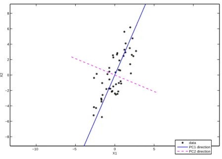
−10 −5 0 5 10 −8

−6 −4 −2 0 2 4 6 8

X1

X2

data PC1 direction PC2 direction

Figure 2.2: Depicts the construction of the PC direction vector. The first direction accounts for most variation of the data and the second direction is orthogonal to the first.

In particular, the m-th eigenvector, vm, is the solution to

arg maxvv0Sv = arg maxvPn_i₌₁(v0xi)2

= arg maxvVar(v0X)

subject to||v||= 1 and v0vl = 0 for l = 1,2,· · · , m−1,

(2.12)

where Var is the shorthand for the variance over the sample. Put in words, the measurements on observations spread out the most along the first PC direction vector

v1 in the d-dimensional space. The second PC direction vector, v2, is the maximal

variance amongst all direction vectors perpendicular to v1 as shown in Figure 2.2.

Note that a unit vectorv orthogonal to the first eigenvectorv1 is alsoSorthogonal

tov1, and vice versa. So, form= 2, if we replace the orthogonality condition,v0v1 = 0,

(28)

the solution of the optimization. The same argument can be used subsequently to show that the m-th eigenvector of S, vm, satisfies

arg maxvVar(v0X)

subject to||v||= 1 andv0Svl= 0 for l = 1,2,· · · , m−1.

(2.13)

The variance of the data along the m-th PC direction is

Var(v0_mX) ∝Pn_i₌₁(x0_ivm)2

=v0_mSvm

=λm.

The amount of variability that can be explained by the direction vm is reflected on

the magnitude of its corresponding eigenvalue. If eigenvalues beyond the m-th are small, we might expect that discarding the principal components corresponding to or beyond the m-th might not lead to loss of too much information.

Principal Component Regression

Principal Component Regression (PCR) (Massy, 1965), regresses the output vari-able onto the first ω PCs, which contain most of the variability in the original input variables. For the choice of ω, Cross-Validation (CV) (Stone, 1974) has been sug-gested as an approach to this (Frank and Friedman, 1993).

(29)

Toy Example

We generate a 2−dimensional regression data set {(xi1, xi2, yi)} of size 50. The

input data, {(xi1, xi2)}, are seen in Figure 2.2. This plot gives an image of how the

regression data {(xi1, xi2, yi)} are distributed in the 2-dimensional input space only.

The movie, Lee (2005b), shows the data{(xi1, xi2, yi)}in the 3-dimensional space,

from a rotating viewpoint. This can be helpful to have a feeling about how the data appear in the 3-dimensional space. Notice that the data appear to spread more along the X2 axis than the X1 axis. As the view angle spins, the data points, sometimes,

appear to lie near a line (correlation ≈ 1), but sometimes they seem to spread very randomly (correlation ≈ 0).

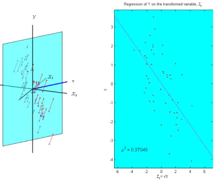
In the movie, Lee (2005c), the viewpoint is fixed, but the direction vector in the

X space, v, denoted as the blue line, is rotating to search for the maximal input data variation vector. Figure 2.3 is a snapshot from this movie. The left panel illustrates how the dimension reduction of the input data can be attained via the linear transformation. The right plot shows the resulting projected data and linear regression. For an arbitrarily chosen direction vector, v, the corresponding linear transformed variable is given as Z1 = v0X. The regression of Y on Z1 now is a

simple linear regression, and the data pairs for this regression analysis are obtained by projecting data on the 2-dimensional face determined by Z1 and Y, which is

denoted as the cyan phase. The projections - denoted as circles - are linked with the original data - denoted as crosses- for i= 1,· · · ,50. For better demonstration of the regression analysis with the transformed variable, the blue plane is extracted and displayed on the right hand side.

The rotation stops at the vector v1 (PC1 direction vector) to maximize the

vari-ation of the input data. One can see that the performance of the regression on the first PC very poor.

(30)

Figure 2.3: Toy Example with 2−dimensional regression data (xi1, xi2, yi)}501 . A

snap-shot from the movie, Lee (2005c). Left: A subspace, represented by the cyan plane, is generated by the arbitrarily chosen direction vector, v, and the output variable,Y. Each data point- blue cross- and its projection on this plane- red circle- are linked together by red lines. Right: The blue plane pulled from the left side. The red dots form the data for the 1-dimensional regression analysis using the transformed variable, v0X as a regressor.

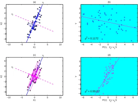
of the input data could be irrelevant to the output variable. On the top left panel, the two PC vectors, v1 and v2 are shown in the input space. Having fixed the direction

(31)

−10 −5 0 5 10 −6 −4 −2 0 2 4 6 X1 X2 (a)

−6 −4 −2 0 2 4 6

−4 −3 −2 −1 0 1 2 3 ρ2 = 0.1172

PC1, Z

1= v1’X

Y

(b)

−10 −5 0 5 10

−6 −4 −2 0 2 4 6 X1 X2 (c)

−6 −4 −2 0 2 4 6

−4 −3 −2 −1 0 1 2 3 ρ2 = 0.55127

PC2, Z₂= v₂’X

Y

(d)

Figure 2.4: Toy Example with the same 2−dimensional regression data (xi1, xi2, yi)}501

as in Figures 2.2 and 2.3. (a) Projection of input data onto the first PC direction vector in the (X1, X2) plane (b) Scatter plot of the first PC against output data (c)

Projection of input data onto the second PC direction vector (d) Scatter plot of the second PC against output data, showing that it is the second PC that carries the important information about the output data (i.e., much stronger correlation with

Y).

2.3.4 Partial Least Squares

Since Partial Least Squares (PLS) introduced by Wold (1976) in an algorithmic form, a variety of different algorithms (Naes and Martens (1985), Helland (1988)) that produce the same solutions have been proposed. It is very popular in the field of chemometrics, where HDLSS settings which often lead to multicollinerity between variables are commonplace.

(32)

specif-ically the m-th PLS direction vector,vm, solves

arg maxvCov2(v0X, Y) = arg maxvCorr2(v0X, Y)Var(v0X)

= arg maxv <Xv,Y>2

= arg maxv(v0s)2

subject to||v||= 1, v0Svl= 0, l= 1,· · · , m−1 wheres=X0Y.

(2.14)

In contrast with the PC direction, the PLS direction is found in connection with the output variable. The first PLS directionv1 maximizes the covariance between the

output variable and the linearly transformed variable, v0X over the data.

An interesting connection among the criteria for OLS in (2.10), PCR in (2.13), and PLS in (2.14) can be found: the criteria for PLS, Corr2(v0X, Y)Var(v0X) is the square of the geometric mean of criterion for OLS and PCR. This suggests that PLS can be regarded as a compromise between OLS and PCR. This point is illustrated in Figure 2.5. With the simulated data that we employed in the previous section, the first OLS, PCR, and PLS vectors are drawn. The PLS vector lies between the OLS and the PCR vectors. Unlike PCA, PLS makes direct use of the information about the output variable, but to a smaller extent than OLS does.

While building up the PLS vectors sequentially, we can add the corresponding factors in the regression analysis as explanatory variables. The Cross Validation criteria is one way to choose the number of PLS factors that needs to be included in the regression (Frank and Friedman, 1993).

2.3.5 Continuum Regression

Continuum Regression (CR) proposed by Stone and Brooks (1990) is a general procedure to reduce a regression model in terms of linear transformations of the original regressors as introduced in (2.6). With a criteria varying with a parameter

(33)

Figure 2.5: Toy Example with the same 2−dimensional regression data {(xi1, xi2, yi)}501 as in Section 2.3.3. The cyan plane stands for the X-space. The

first direction vectors for OLS, PLS, and PCR are drawn. The OLS direction is nearly orthogonal to the PCR direction, and the PLS direction lies between the OLS and the PCR directions.

regressors embrace OLS, PLS, and PCR.

(34)

sequentially to maximize

T(α) = Cov2(v0X, Y)Var(v0X)α/(1−α)−1

= (v0s)2₍_v0_S_v₎α/(1−α)−1

subject to ||v||= 1 andv0Sv_l0 = 0 for l = 1,· · · , m−1.

(2.15)

Here, Cov and Var are the sample covariance and sample variance over the data. For

α= 0,

arg max

v T(0) = arg maxv Cov

2₍_v0

X, Y)Var(v0X)−1 = arg max

v Corr

2₍_v0

X, Y).

Forα = 1/2,

arg max

v T(

1

2) = arg maxv Cov

2₍_v0

X, Y).

Clearly, CR for α = 0 and α = 1₂ corresponds to OLS and PLS, respectively. The PCR, however, can be understood only in the limiting sense as α →1. But, we can not expect that PCR is always the limit of CR as α goes to 1. In particular, even though the function (2.15) is continuous with respect to α, it is not generally true that the maximizer,v(α)∈_Rd_{, as a function of}_α_{, is also continuous with respect to}

α. Bj¨orkstr¨om and Sundberg (1996) demonstrates that CR can yield a discontinuous maximizerv(α), as a function ofα.

Having found the direction vector, vm(α) at the m-step for a fixed value ofα, the

linearly transformed regressor, v_m0 X is added to the regression analysis. Thus, the CR procedure gives rise to a set of linearly transformed regressors,

{(v1(α)0X,· · · , vω(α)0X)|α∈[0,1],16ω6M}, whereM = rank (X).

(35)

Cross-Validation error is suggested by Stone and Brooks (1990).

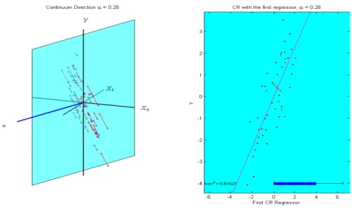
Toy Example

Figure 2.6: Toy Example with the same 2−dimensional regression data (xi1, xi2, yi)}501

as in Section 2.3.3. Left: The CR direction vector for a given α is found and plotted as the blue line. The projections of input data on this direction, in pairs of output data, are plotted as red circles. Right: The blue plane from the left hand side shows the CR on the corresponding CR factor.

Using the same data as in Section 2.3.3, the first direction and the corresponding first factor of CR are calculated as a function of α in the movie, Lee (2005d). Figure 2.6 is a snapshot of this movie. Data pairs, (xi1, xi2, yi) are shown as crosses in the

3-dimensional space. For a fixed value of α, the direction vector, v, maximizing the objective function in (2.15) is found and represented as the blue line. By projecting the input data (xi1, xi2) onto this direction vector, we obtain the first CR factor,

(36)

CR on the first factor. The blue thick bar at the bottom indicates the magnitude of the sample correlation between the output variable and the first CR factor. This movie shows the full span of the CR vectors from the OLS vector to the PCR vector.

2.4 Application to Microarray Data

This example involves a large input data set with n = 36 mouse samples and

d= 17000 gene expression measurements from microarrays. The microarray measures mRNA abundance which is used to derive the level of expression for thousands of genes simultaneously. Since the activity of a gene, represented by the quantity of mRNA, reflects the molecular status of the sample, gene expression profiles can be used to classify the different subtypes of disease. There have been many attempts to adapt statistical tools for discrimination/ clustering for performing this type of diagnosis. When we have an accompanying variable that characterizes the same samples, such as survival time or other quantitative measurements, a common statistical task is to build a prediction model that uses the gene expression level, for a sample as input to predict the output value.

CR can be seen as a method to unify these two types of tasks in a way that solely unsupervised (PCR) and solely supervised (OLS) tasks occupy the two ends of the CR spectrum and that puts an interesting range of intermediate methods, (e.g. PLS), between them.

For this example, the maximizer direction vector will be computed for each value of

α= 0, .1,· · · ,1. Entries of a direction vector can be interpreted as the contribution of genes on the particular direction vector. Sorting the entries of each direction vector in an decreasing order gives the rank of gene contributions on each direction vector. Note that genes with the largest positive (negative) entries are the ones which influence most on the given direction vector.

(37)

lab in Section 2.4.1. In Section 2.4.2, we will use the continuum parameter, α, in a novel way, to study how gene ordering changes over theαspectrum by creating “rank tracking plots”. To identify biologically relevant genes, the tracking visualization will be used in a different way in Section 2.4.3.

2.4.1 Experiment and Data

A mouse experiment was conducted in the Rusyn lab to study the genetic factors affected by exposure to alcohol that may contribute to liver disease. A panel of six inbred mouse strains (A/J, AKR/J, BALB/cJ, C3H/HeJ, C57BL/6J, and DBA/2J) was exposed to alcohol acutely as a bolus of 5g/kg intra-gastric dose for 6 hours. Liver and blood was taken from the alcohol-treated mice and controls to assess several measurements. Several phenotypic changes (associated with alcohol toxicity in liver) were measured from control and alcohol-treated mouse samples. In addition to that, gene expression profiling was performed from the mouse samples above.

For the application of CR, we consider the d genes in the microarray as input variables, (X1,· · · , Xd), and the Blood Alcohol Concentration (BAC), a continuous

phenotype, as the response variable, Y.

(38)

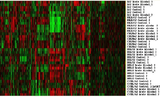
Figure 2.7: Heat map view of Gene Expression from 36 mouse samples. Columns represent genes (variables) and rows display gene profiles from samples (observation). Note that transposing this map is the usual way of displaying. We take this view because the mouse strain labels on the right are clearly labeled.

each other. This indicates that the strain factor dominates the treatment factor. Also, note that all the alcohol-treated samples and the control samples within a strain are clustered next to each other except for one strain, A/J. This indicates that this experiment is very replicable. Genes with similar expression patterns are also clustered together. In the middle, one can see a vertical stripe pattern- bright greens for BALB/CJ, reds for the bottom three strains (DBA/2J, AKR/J, and C57BL/6J) and somewhat green for the rest of two strains (A/J, C3H/HeJ). This stripe pattern seems to dominate other patterns of genes.

(39)

pointed out in the paragraph above, one can clearly see that the strain, BALB/CJ, is far from the rest of the strains in the projection plot on the 1st PC. In the 2nd diagonal plot, the circles (controls) and crosses (acute treatments) are nicely separated. This shows that the treatment factor also explains the variability across the samples, having adjusted the variability by the first PC. Off-diagonals are 2-dimensional projection plots on the subspaces spanned by each pair of the 4 PC directions. For example, the plot on the top and the second from the left is the projections of the expressions on the subspace generated by PC1 and PC2 direction vectors. From the 2-dimensional projection plots, one can see that

1. the same colors (strains) tend to be close to each other

2. within each color cluster, samples are grouped as symbols (treatments)

The main lessons from the PCA scatter plot are similar to the lessons from the heat map, but some patterns are more clear through appropriate low dimensional projections.

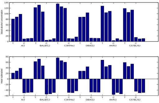
The top panel in Figure 2.9 is the bar-graph of the blood alcohol concentration (BAC) data (Y) from the samples with the microarray data and the bottom the sample-mean subtracted BAC data. The bottom panel shows the distribution of phenotypes across the mouse samples. The main variability clearly is due to treatment effect. Note that, however, variability across strains within alcohol-treated samples is noticeably bigger than variability in the control. This means that the phenotypes are affected by genetic differences. OLS, a way to associate expression data with phenotypes, clearly differs from the discrimination study in the sense that it takes into account the strain variability within treatment/contol samples.

2.4.2 CR Analysis

(40)

−20 0 20 40 0 0.005 0.01 0.015 0.02 PC1

A/J AKR/J BALB/CJ

−20 0 20

0 0.005 0.01 0.015

PC2

−200 0 20

0.01 0.02 0.03 0.04

PC3

−20 0 20

0 0.005 0.01 0.015 0.02 PC4

−20 0 20

−20 0 20 40 PC2 PC1

C3H/HeJ C57BL/6J DBA/2J

−20 0 20

−20 0 20 40 PC3 PC1

+: Treatment o: Control

−20 0 20

−20 0 20 40 PC4 PC1

−20 0 20 40

−20 0 20

PC1

PC2

−20 0 20

PC3

PC2

−20 0 20

PC4

PC2

−20 0 20 40

−20 −10 0 10 20 PC1 PC3

−20 0 20

−20 −10 0 10 20 PC2 PC3

−20 0 20

−20 −10 0 10 20 PC4 PC3

−20 0 20 40

−20 −10 0 10 20 PC1 PC4

−20 0 20

−20 −10 0 10 20 PC2 PC4

−20 0 20

−20 −10 0 10 20 PC3 PC4

Figure 2.8: PCA Scatter plot of Gene Expression data. Colors and symbols indicate strains and treatments, respectively. Diagonals are 1-dimensional projections on the first 4 PC directions and off-diagonals are 2- dimensional projections on the subspaces generated by those directions.

seen as a contribution of the corresponding gene on the first CR vector. Suppose, for example, the first CR vector forα= 1, i.e., the first PC vector, isv1(1) = (1,0,· · · ,0).

An interpretation of this is that the first gene explains the most variability in the samples, whereas the rest of the genes contribute nothing to the directions of the largest variability. We will use the continuum parameter, α, in a novel way, to study loadings simultaneously over α∈[0,1].

(41)

T C T C T C T C T C T C 0

20 40 60 80 100 120 140

blood alcohol concentration

A/J BALB/CJ C3H/HeJ DBA/2J AKR/J C57BL/6J

T C T C T C T C T C T C

−60 −40 −20 0 20 40 60 80

mean subtracted

A/J BALB/CJ C3H/HeJ DBA/2J AKR/J C57BL/6J

Figure 2.9: The bar graph of the output data, Blood Alcohol Concentration. Mouse samples (x-axis) are grouped as strain (A/J, ..., C57BL/6J) and within a strain, alcohol-treated(T)/ control (C) samples are grouped together. We see an obvious effect by alcohol treatment and some variability between mouse strains.

Figures 2.10 and 2.11 show the rank tracks (over the continuum parameter, α) of the 100 largest positive and negative valued genes for the OLS direction (α = 0) over α = 0,0.1,· · · ,1. Based on OLS, we select those top ranked genes (100 largest positive and 100 largest negative), i.e. genes that feel the phenotype differences across the samples. Then, we keep track of their ranks based on CR direction vectors as the continuum parameter,αmarches along the range with increments .1. It is interesting to see when the top ranked genes on OLS disappear. Most genes stay influential until

(42)

0 0.1 0.2 0.3 0.4 0.5 0.6 0.7 0.8 0.9 1 100

90 80 70 60 50 40 30 20 10 1

keep track of indices of top 100 genes from OLS

Figure 2.10: Rank tracking plot of the top 100 ranked genes from OLS (α = 0). Most genes stay highly ranked until α goes to 0.5 (PLS). Afterwards, a portion of genes disappear (low ranked) as we get closer to PCR and none of the genes survive at the very end, α= 1 (PCR).

PLS, a compromise between the OLS and PCA, is in fact, much closer to the OLS in this example.

2.4.3 Loading Tracking Plot

In this section, we will use the loading tracking visualization in a really different way. Instead of comparing CR direction vectors over α, we now consider different direction vectors. In addition to OLS and PLS, direction vectors considered in this section include several important discrimination methods. We view the loadings (entries) of the direction vector as gene contributions to the direction vector. The loading tracking visualization nicely conveys the changes in relative gene contribution as the direction vector changes.

(43)

0 0.1 0.2 0.3 0.4 0.5 0.6 0.7 0.8 0.9 1 −1

−10 −20 −30 −40 −50 −60 −70 −80 −90 −100

keep track of indices of bottom 100 genes from OLS

Figure 2.11: Rank tracking plot of the bottom 100 ranked genes from OLS (α= 0). About half of genes appear to be highly ranked untilαreaches 0.9 and all genes but 3 genes suddenly disappear whenα = 1. Genes responsible for the PC direction, which explains the most variability in the samples, could be very different from the genes relevant to the response variable (α= 0).

the 1-dimensional projection on the first PC (first diagonal in Figure 2.8) shows that most of the variability comes from strain differences. On the other hand, the second most variability is mainly due to the treatment effect as seen in the second diagonal. Genes that drive the treatment effect are of more interest than genes that drive strain differences. For this reason, the second PC is considered rather than the first PC in the following analysis.

A more direct approach for identifying genes that are expressed differently between the treatment and control groups is discrimination. Discrimination methods, and also their use in the analysis of expression data, have been widely studied by many researchers. See Hastieet al. (2001), Dudaet al. (2000), Tibshirani et al.(2003) and references therein.

(44)

Discrimi-nation (DWD) proposed by Marron et al. (2007) since it performs reasonably well in HDLSS contexts. See Marron et al. (2007) for details. We also consider Mean Difference (MD, also called centroid by Tibshiraniet al. (2003)), an especially simple discrimination method. MD is the normalized vector of the gene expression mean difference between the control and treatment groups.

PC PLS OLS DWD MDP

−0.1 −0.05 0 0.05 0.1 0.15

Direction Vector Entries

Figure 2.12: loading tracking plot for 5 direction vectors- the 2nd PC, PLS, OLS, DWD, MD. Each gene is represented by a piecewise line, connecting the entries of the respective directions. A few genes stand out as important across all the methods.

Sorting genes based on different direction vectors suggest different lists of impor-tant genes. Genes having large loadings in the second PC direction are the ones that explain the second most variability across the samples in the gene expressions (which might be related to treatment effect as explained above) . DWD and MD (right ends) are useful to identify genes that differentiate the alcohol treated sample from the con-trols. With OLS (the central ordinate), genes that best explain the phenotype, BAC, can be obtained.

(45)

these tasks. For each gene, we keep track of entries as the direction changes (from the second PC to PLS, OLS, DWD, and MD). These form a piecewise line in Figure 2.12, which shows the change of gene loadings for the five different direction vectors. Most of the loadings are between -.05 and .05 whereas there are some genes stand-ing out for some particular methods, or across all the analyses. The thick bundle of black curves in the middle hinders understanding as to whether they are actually par-allel or crossed (up in one analysis, but down in the other, or vice versa). However, genes with low loadings (in absolute value) for all ordinates are not related to the treatment. A few genes stand out across all the methods, and these are worth looking at in detail.

PC PLS OLS DWD MD

−0.1 −0.05 0 0.05 0.1 0.15

Direction Vector Entries

Figure 2.13: loading tracking plot, with several genes of interest highlighted. The 50 top genes based on the absolute value of OLS are colored as red, 50 based on DWD colored as blue, and purple for genes selected by both.

(46)

−0.06 −0.04 −0.02 0 0.02 0.04 0.06 0.08 0.1 0.12 0.14 −0.1

−0.05 0 0.05 0.1 0.15

OLS

DWD

highlighted genes having largest |ols|, |dwd|, or both

* : |ols|

* : |dwd|

* : both

Figure 2.14: Scatter plot of OLS and DWD gene loadings. Genes are distributed along the 45◦, which indicates OLS and DWD loadings strongly correlated. The 50 top genes based on the absolute values of the OLS are colored as red, 50 based on DWD colored as blue, and purple if selected by both.

(47)

Analyzing the gene loading changes that correspond to the black lines is challeng-ing as the visualization is obscured by the thick bundle of lines in the middle. To focus on the comparison of OLS and DWD only, we create a scatter plot of entries for these two vectors in Figure 2.14. This scatter plot shows the loading distribution over the two direction vectors. Genes are distributed along the 45◦ line with some variations, i.e., some genes have larger loadings in OLS than DWD, and vise versa. However, the 45◦ line pattern is pretty clear, which indicates that the gene contributions to OLS and DWD are strongly correlated with each other.

(48)

CHAPTER 3

Continuum Canonical Correlation

There are cases where two sets of multidimensional variablesX = (X1,· · · , Xd1)T

and Y = (Y1,· · · , Yd2)T, are observed in pairs

{(xi,yi)| xi ∈Rd1,yi ∈Rd2, i= 1,· · · , n}

and the distinction between explanatory variables and response variables are not so clear. In that case, analysis dealing with two sets of variables in a symmetric manner would be more appropriate than the regression type analysis, done in this context by Stone and Brooks (1994).

Canonical Correlation Analysis (CCA), proposed by Hotelling in (Hotelling, 1936), is an example of this type of analysis. CCA is a method of finding linear relationships between two multi-variables. CCA seeks for two direction vectors, one for each vari-able set, such that the sample correlation between the projections of the data onto those two direction vectors are maximized.

In this chapter, we propose a generalization of CR, studied in Chapter 2, for two sets of multivariate data cases. The new method will be obtained by extending CCA into a family of CCA type analyses. Hence it will be called Continuum Canonical Correlation(CCC). CCC bears resemblance with CR in that

(49)

(ii) several existing methods such as Canonical Correlation Analysis (CCA), PLS (maximal covariance direction), and PCA, which we will study more in detail later in this chapter are special cases.

However, CCC differs from CR in that direction vectors in both sets of variables are of explicit interest.

In Section 3.1, we will give the description of the new method CCC. Three special cases of CCC will be reviewed in the later sections; CCA, the maximum correlation method in Section 3.3, PLS, the maximum covariance method in Section 3.4, and the PCA, the maximum variance method in Section 3.5. CCA (α= 0) and PCA (α = 1) occupy the ends of the spectrum of the new method and PLS (α= 1/2) lies in the mid-dle. These three special methods can be put in a common mathematical framework, and solved as a generalized eigenvalue problem (Borga et al. (1997), Shawe-Taylor and Cristianini (2004)). In Section 3.2, the generalized eigenvalue problem will be described. A numerical algorithm to find CCC direction vectors for general values of

α∈[0,1] is proposed in Section 3.6.

3.1 Continuum Canonical Correlation

Define the two data matrices as Xd1×n := [x1,· · ·,xn] and Yd2×n:= [y1,· · · ,yn].

The direction vectors,um ∈Rd1 andvm ∈Rd2, are taken as the following maximizer:

T(α) = max

u∈Rd1,v∈Rd2

{Cov(uTX,vTY)}2{Var(uTX)Var(vTY)}α/(1−α)−1

= max

u∈Rd1,v∈Rd2

(uTXYTv)2(uTXXTuvTYYTv)α/(1−α)−1 (3.1)

where 0₆α <1 subject to uT

mum =vmTvm = 1, uTmXXTuj = 0 and vmTYYTvj = 0

for j = 1,· · · , m−1.

(50)

max-imization problem indexed by the free parameter, α, but differs in that it finds two direction vectors, one for each variable setX andY. As for CR, CCC also embraces 3 existing methods: CCA, PLS, and PCA. These three special cases can be formulated as generalized eigen-problems, which will be introduced in the following section. In Sections 3.3 - 3.5, CCA (α = 0), PLS (α = 1/2), and PCA (α →1) will be studied in detail.

3.2 The Generalized Eigenproblem

Following the development in Chapter 6 of Shawe-Taylor and Cristianini (2004), the generalized eigenproblem will be reviewed in this section. The generalized eigen-problem is closely related to the eigen-problem of finding the maximum point of a ratio of quadratic forms

r= w

T_Aw

wT_Bw

where A and B are both symmetric and B is positive definite. This ratio is known as the Rayleigh quotient. Taking the derivatives with respect to w and setting them to zero gives the equation:

∂r

∂w =

2

wT_Bw(Aw−rBw) = 0

or equivalently the generalized eigenproblem:

Aw=rBw. (3.2)

Since by assumptionBis positive-definite, by pre-multiplying the equation withB−1, we can covert (3.2) to an ordinary eigenproblem

(51)

Letr1 >· · ·>rm be the eigenvalues of B−1A and w1,· · · ,wm be the corresponding

eigenvectors.

It can be shown that (Shawe-Taylor and Cristianini (2004), Borga et al. (1997)) the eigenvector corresponding to the maximum (minimum) eigenvalue, w1(wm), is

the global maximum (minimum) point of the Rayleigh quotient and the remaining eigenvectors are saddle points. Therefore, searching for the maximum point of the

Rayleigh quotient (3.2) is equivalent to finding the eigenvector of the generalized eigen-problem (3.2) corresponding to the largest eigenvalue. It is useful to view the generalized eigenproblem from a sequential viewpoint. After the eigenvector corre-sponding to the largest eigenvalue,w1, is computed, the eigenvector corresponding to

the second largest eigenvalue, w2, solves the following maximization problem under

an orthogonality condition:

w2 = argmaxw:wT_Bw

1=0

wT_Aw

wT_Bw.

A similar sequential representation holds for the remaining eigenvectors. Thus, the solution of the generalized eigenproblem gives a sequence of direction vectors to max-imize the Rayleigh quotient in (3.2) under theB-orthogonality condition.

In the following sections, we will see that CCA, PLS, and PCA can be formulated as a generalized eigenproblem, with a special choice of the matrices A and B.

3.3 CCA: Direction of maximum Correlation

(52)

The empirical correlation between Z :=uT_X _and _W _:=_vT_Y _{can be written as}

ρ =. _p Cov(Z, W)

Var(Z)pVar(W)

= u

T_XYT_v

√

uT_XXT_u√_vT_YYT_v. (3.3)

Note that this corresponds to the CCC when α = 0. Since the correlation is scale invariant, the vectors u and w are determined up to direction. The requirement uT_XXT_u ₌ _vT_YYT_v _{= 1 can resolve the ambiguity of scale issue. Then, CCA is}

equivalent to the following:

maxu,vuTXYTv

subject to uTXXTu=vTYYTv= 1.

The corresponding Lagrangian is

uTXYTv− λx 2 (u

T

XXTu−1)− λy 2 (v

T

YYTv−1).

Taking the partial derivatives with respect tou and v, and setting the derivatives to zero give the equations,

n XYTv=λ_xXXTu

YXT_u₌_λ

yYYTv.

(3.4)

Subtracting uT _{times the first from} _vT _{times the second, we obtain} _λ

xuTXXTu−

λyvTXXTv= 0, which implies λx =λy. Denoting this value by λ and letting

A=

0 XYT

YXT ₀

, B=

XXT 0

0 YYT

, and w=

u v

, (3.5)

(53)

will give the canonical direction vectors,u1andv1. The maximum of the correlationρ

overuandvis called thecanonical correlation, and the linearly transformed variables

Z =uT

1 X and W =vT1 Y are called canonical variates.

3.3.1 Example

In the movie, (Lee, 2005a), the canonical directions are studied for a d1 =d2 = 2

example, using simulated data. Figure 3.1 is a snap shot from the movie. The top panel on the left shows the X data as black stars, and the projections of data, onto one arbitrarily chosen direction vector u, as red circles. The bottom panel is for the

Y data and another arbitrary v. The panel on the right shows the scatter plot of the paired projections, onto the 2-d subspace of _R4 _{generated by the direction vectors} _u

and v, which shows a weak correlation for this choice of u and v.

In the first part of the movie, the direction vector u in the X space is fixed as shown in Figure 3.1, and the direction vector v in the Y space is rotated. As the direction rotates, the joint distribution of the projections in the right panel changes. Rotation stops at the direction v1 which gives the maximum correlation. In the

second part of the movie, v1 in the Y space is fixed, and direction vector in the X

space is rotated. Similarly, rotation stops at the vectoru1 to maximize the correlation

of the paired projections.

Figure 3.2 is the last snap shot from this movie. The panel on the right shows the scatter plot of data projections onto CCA direction vectors, which clearly shows a strong linear correlation. Note that the CCA vectors, u1 and v1, indicated by

blue lines on the left, are nearly orthogonal to the PCA vectors, in each of X and Y

(54)

−5 0 5 −2

−1 0 1 2

X1

X2 u

−3 −2 −1 0 1 2 3

−1.5 −1 −0.5 0 0.5 1 1.5

Y1

Y2

v

−3 −2 −1 0 1 2 3

−2.5 −2 −1.5 −1 −0.5 0 0.5 1 1.5 2 2.5

Scatter plot of projections

Projections of X data onto direction u

Projections of Y data onto direction v

ρ = 0.46097

Figure 3.1: Two paired sets of 2-d data vectors and the projections of the two direction vectors are shown in the left panels. The scatter plot of data projections are seen in the right panel. This show a weak correlation between the paired projections.

3.3.2 HDLSS CCA

For HDLSS data in the sense that either d1 > nord2 > nholds, or both hold, the

matrix B in the equation (3.5) becomes singular. An ordinary approach to solving the eigenvalue problem by pre-multiplying the inverseBon both sides of the equation can not be applied. For the sake of simplicity, assume for now that only d1 > n is

true. Then, the rank of the covariance matrix XXT _{is less than its dimension} _d 1.

In particular, this means that null space {u | uT_XXT_u _{= 0}} _{is not empty. For}

(55)

−5 0 5 −2

−1 0 1 2

X1

X2

u₁

−3 −2 −1 0 1 2 3

−1.5 −1 −0.5 0 0.5 1 1.5

Y1

Y2

v₁

−3 −2 −1 0 1 2 3

−2.5 −2 −1.5 −1 −0.5 0 0.5 1 1.5 2 2.5

Scatter plot of projections

Projections of X data onto direction u₁

Projections of Y data onto direction v

1

ρ = 0.75832

Figure 3.2: Two paired sets of 2-d data vectors and the projections of the CCA direction vectors are shown in the left panels. The scatter plot of data projections onto CCA vectors are seen in the right panel, which clearly shows a strong correlation.

is 0, thus the ratio is undefined. Therefore, for a singular covariance matrix XXT_,

maximizing the correlation is not well- defined. This is true in all of the casesd2 > n,

or both d1 > n and d2 > n are true.

To circumvent the singularity problem, confine the direction vectors to be in the subspace generated by the data, i.e., u = Xα and v = Yβ for some α ∈ _Rn _and

β ∈_Rn_{. Substituting into the equation (3.3) we obtain the following}

ρ= α

T_XT_XYT_Y_β

√

(56)

Assume Rank(XT_{X) =} _n _{and Rank(Y}T_{Y) =} _n_{. Then, the maximization problem}

over α and β is now well defined. As for the ordinary CCA, it can be formulated as a generalized eigenvalue problem.

3.4 PLS: Direction of maximum Covariance

PLS is a widely used method in chemometrics when tackling a regression problem. The PLS begins with canonical covariance analysis; maximize the covariance between projections of two paired sets of data onto two directions specified byuand v. There are several versions of PLS for the multiple response case; they differ in the way that orthogonality constraint for subsequent direction vectors is imposed (Phatak and Jong, 1997). In this work we stick to a particular version of PLS introduced in Borgaet al. (1997).

The set of vectors are obtained in pairs and we are interested in studying the covariance between the two parts of the paired data set. This is in contrast to the CCA which normalizes with respect to the variances of two linear combinations, thus studying correlation. The directions u and v of maximum covariance can be formulated as follows:

max

u,v Cov(u T

X,vTY) = max

u,v u T

XYTv

subject to uTu= 1 andvTv= 1.

(3.6)

The objective function is the same as that of CCC for α= 1/2. Applying the La-grange multiplier technique to the maximization problem (3.6) gives the optimization problem

max

u,v u T

XYTv− λx 2 (u

T

u−1)− λy 2 (v

T

v−1).

Continuum direction vectors in high dimensional low sample size data