ON THE QUANTUM TYPE C SPIDER
Logan Tatham
A dissertation submitted to the faculty at the University of North Carolina at Chapel Hill in partial fulfillment of the requirements for the degree of Doctor of Philosophy in the Department of
Mathematics in the College of Arts and Sciences.
Chapel Hill 2020
Approved by:
David E.V. Rose
Cris Negron
Richard Rimanyi
Lev Rozansky
ABSTRACT
Logan Tatham: On the Quantum Type C Spider (Under the direction of David E.V. Rose)
In this thesis, we make significant progress towards finding a diagrammatic description of
the categoryRep(Uq(sp2n)) of representations of the quantum groupUq(sp2n). A diagrammatic description ofUq(g) for other Lie typesg is known:
g=sl2 (Rumer-Teller-Weyl 1932)
g=sl3,sp4,g2 (Kuperberg, 1996)
g=sln (Cautis-Kamnitzer-Morrison, 2012)
but beyond this, nothing is known. Diagrammatic descriptions ofUq(g) are useful for many reasons, including a diagrammatic description of the Reshetikhin-Turaev link invariants, which then lend
towards categorification.
In this work, we introduce a diagrammatic category Web(sp6) which we conjecture is equivalent to the category of tensor products of fundamental Uq(sp6) representations, FundRep(Uq(sp6)). We define a functor Web(sp6)→FundRep(Uq(sp6)) which is full and essentially surjective, and conjecture that it is faithful. Further, we prove that Web(sp6) satisfies some necessary properties of being equivalent toFundRep(Uq(sp6)), including having the correct categorical trace and that EndWeb(sp6)(∅) =C(q) (where ∅is the monoidal unit of Web(sp6)). We also define a braiding on
To May Priegel, for her unwavering love and support. To my family, for their unwavering love. To everyone who has had similar struggles as me in
ACKNOWLEDGEMENTS
I would like to say thank youto the following people:
My excellent advisor, David Rose, for so much invaluable help in this work, without which,
none of this would be possible. I’m glad he took a risk on me by picking me as his first student,
especially when there were so many other strong students he could have taken. For doing
more than just pushing me when I needed it, but also being sensitive and patient with me
when I needed that. And finally, for giving me quite a bit of freedom in choosing what to
research; I hope he will forgive me for the lack of categorification in this work!
My partner, May Priegel, for her unwavering love and support, not only with my research,
but of everything I do, and for always believing in me.
My parents, Kim and Glen Larson, for giving me a great home while growing up, and for
always being willing to listen to me while I went through challenges.
My grandparents, Dale and Mary Ellen Peterson, for giving me a great childhood and teaching
me how to work and feel confident.
My birth dad, Rich Tatham, for helping me have a great childhood and for being inspirational
to me in turning his life around.
My siblings, Lindsay, Lexy, Liberty, for being some of my best friends throughout my life, and
for knowing me so well.
My friends Russell Ollerton, Spenser Squire, for introducing me to yerba mate and being my
best friends.
Alex Safsten, Erica Kiefer, Zac Lowell.
Russ Arnold, Austin Ferguson, Sam Jeralds, Gonzalo Cazes, Dmitro Golovonich, Marc Besson,
Bill Reel and Radio Free Mormon, for their excellent podcasts which gave me support and
clarity in areas no one else could. They both feel like close friends.
The math and economics departments at Brigham Young University, especially Denise
Halver-son and James McDonald for their research mentorship.
The department of math at the University of North Carolina at Chapel Hill, for fostering a
great environment in which to do graduate work.
All the other schools I’ve attended, but especially Jollyville Elementary and their Special
Education program.
UNC CAPS.
The countless undergrads at UNC who gave me extra meal swipes, which amounted to me
having free lunch and dinner almost daily for about 3 years
Duke Cannon, for sending me free stuff because I emailed them and asked them to.
I would like to say no thank youto the following:
The current worldwide coronavirus pandemic, for infecting too many of my family members.
That time I broke my tooth on a smoothie and it cost me a ton to fix it.
That time a bus ran into my legally parked and stationary car.
That time a health clinic erroneously charged me a small fortune for a treatement I had
TABLE OF CONTENTS
LIST OF FIGURES . . . ix
LIST OF TABLES . . . x
CHAPTER 1: INTRODUCTION . . . 1
CHAPTER 2: BACKGROUND . . . 5
2.1 Knots, Links, and the Jones Polynomial . . . 5
2.2 Quantum Groups . . . 9
2.3 Examples ofFundRep(Uq(g)) . . . 14
2.3.1 FundRep(Uq(sl2)) . . . 14
2.3.2 FundRep(Uq(sp4)) . . . 16
2.3.3 FundRep(Uq(sp6)) . . . 18
2.4 Monoidal Categories . . . 24
2.5 Temperly-Lieb . . . 35
2.6 Web categories . . . 39
CHAPTER 3: Ψ :WEB(sp6)→FUNDREP(UQ(sp6)) IS WELL-DEFINED . . . 42
3.1 The braiding onWeb(sp6) . . . 53
CHAPTER 4: WEB(sp2n) AND THE BMW ALGEBRA . . . 56
CHAPTER 5: FULLNESS OF Ψ :WEB(sp6)→FUNDREP(UQ(sp6)) . . . 63
CHAPTER 6: LAD(sp6). . . 66
CHAPTER 7: TR(WEB(sp6)) . . . 74
CHAPTER 9: BRANCHING FUNCTORS AND WEBS . . . 86
9.1 Two functorsWeb(sp4)→Web(sl2)⊕ . . . 87
9.2 A functor Web(sp6)→Web(sp4)⊕. . . 93
CHAPTER 10:TYPE C LINK INVARIANTS . . . 98
CHAPTER 11:FURTHER WORK . . . 100
APPENDIX A: APPENDIX . . . 102
A.1 Relations inLad(sp6) . . . 102
LIST OF FIGURES
LIST OF TABLES
2.1 The fundamentalUq(sl2) representation . . . 15
2.2 The fundamentalUq(sp4) representation V . . . 16
2.3 The fundamentalUq(sp4) representation W . . . 17
2.4 The fundamentalUq(sp6) representation V . . . 19
CHAPTER 1
Introduction
The goal of this thesis is to find a diagrammatic description of the category of representations of
the quantum group Uq(sp6). This can be viewed as a categorical analogue of finding a presentation of a group via generators and relations. This problem has been solved in other types. There exist
diagrammatic presentations ofFundRep(Uq(g)) in the cases:
g=sl2, [29], 1932
g=sl3,sp4,g2 [17], 1997
g=sln [4], 2012.
It has remained a difficult open problem to extend these results to other Lie types. In this work,
we make the first substantial progress towards solving this problem in other types. We begin by
summarizing our results before detailing the relevant background in Chapter 2. We define a category
Web(sp6) which we conjecture is equivalent to the category of (direct sums of tensor products of) fundamental Uq(sp6) representations,FundRep(Uq(sp6); we further prove a number of results in support of this conjecture.
Our categoryWeb(sp6) is presented using diagrammatic language for monoidal categories, which is reviewed in Section 2.4; it is the (strictly pivotal)C(q)-linear category generated by the self-dual
objects{1,2,3} and with morphisms generated by
1 1 2
∈HomWeb(sp6)(1⊗1,2) ,
1 2
3
modulo the relations:
=−[3][8]
[4] , = 0 , =−[2][3] , =−[3]
2 , =
= 0 , = [3]2 + 1
[2] −[3]
− = [2]
−
, − = [2] −
!
We prove that there is a functor
Ψ :Web(sp6)→FundRep(Uq(sp6))
which sends object ito the fundamental representation with highest weightωi, and morphisms to certain module maps defined in Section 2.3. While we have not yet proved that Ψ is an equivalence
of categories, we have proved thatWeb(sp6) satisfies many necessary properties of being equivalent toFundRep(Uq(sp6)). These are:
1. The functor Ψ is full and essentially surjective
2. There is a functor fromWeb(sp6) to (matrices of)Web(sp4) giving a combinatorial analogue of the restriction functorRep(Uq(sp6))→Rep(Uq(sp4)) arising from the inclusionUq(sp4),→ Uq(sp6).
3. There are representations of the BMW algebra (which is “Schur-Weyl dual” [10] to the
endomorphism algebras of the vector representation) to endomorphism algebras inWeb(sp2n). 4. The category Web(sp6) is ribbon, and Ψ is a braided monoidal functor.
5. The functor Ψ induces an isomorphism Tr(Web(sp6))∼= Tr(Rep(Uq(sp6))).
6. dim EndWeb(sp
6)(∅) = 1, so Ψ is faithful when restricted to the monoidal unit∅.
Putting facts (3), (5), and (6) together, we obtain an explicit local construction of the quantum sp6
link invariant, akin to the Kauffman bracket formulation of the Jones polynomial.
hope for a presentation of the category Rep(Uq(sp6)) of all irreducible, finite dimensional Uq(sp6) representations. However, we would prefer a finite presentation, and a description ofRep(Uq(sp6)) has infinitely many generating objects! While FundRep(Uq(sp6)) does not contain every irre-ducible finite dimensional Uq(sp6) representation, any such representation is the highest weight irreducible summand of a tensor product of finitely many fundamental representations, so in a sense,
FundRep(Uq(sp6)) has enough to “see” everything inRep(Uq(sp6)). In fact, there is a process to make this formal, called the Karoubi (or idempotent) completion, and we indeed have
Kar(FundRep(Uq(g))) =Rep(Uq(g))
where Kardenotes the Karoubi completion.
Of course, one may ask why diagrammatic descriptions of FundRep(Uq(g)) is useful. Due to Reshetinkin-Turaev [26], FundRep(Uq(g)) can be used to construct link invariants in S3, so FundRep(Uq(g)) is braided. For example, when g=sl2, this gives a diagrammatic description of the Jones polynomial [13]. While extending this to other types may be enough motivation, there is
an added benefit of a diagrammatic description.
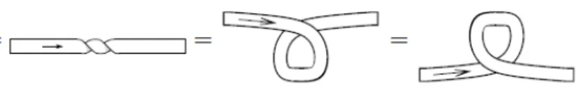
One old problem of knot theory is the Tait conjecture, posed by Tait in the 1880’s [18]. While
tabulating knots, he noticed that alternating knot diagrams (meaning diagrams in when, when a
strand is followed, it alternates going over and under a crossings) seemed to be minimal; that is,
have a minimal number of crossings. This led him to ask if an alternating diagram of a knot is
always minimal. As stated, the answer is no; for example, the knot diagram
is alternating, but not minimal since it represents the unknot. However, loosely speaking, if we
don’t have cases where we can “obviously” untwist the diagram to untwist a crossing, then the
answer is yes. The Jones polynomial was introduced in 1984, but once the diagrammatic description
of the Jones polynomial was introduced by Kauffman in 1987, the Tait conjecture was proved
independently by Kauffman, Murasugi, and Thislewaite [12] [33] [22].
to categorify the Jones polynomial. Specifically, given a linkLwith diagram LD, we may take the homology Kh(L) of a certain (bounded) chain complex of graded vector spaces which then satisfies
Vq(L) =χ(Kh(LD))
where Vq denotes the Jones polynomial andχ denotes the Euler characteristic. (In fact, Kh is an invariant of links, so we perhaps ought to write Kh(L) rather thanLD). The construction of the chain
complex arising fromLD depends heavily on the diagrammatic presentation of FundRep(Uq(sl2)). While the Jones polynomial is a strong invariant, Khovanov homology has been shown to contain
even more topological information. For example, Khovanov homology is an unknot detector, meaning
Kh(L) = Kh(O) if and only if L ∼O (whereO denotes the unknot; it remains an open question as to whether this is true for the Jones polynomial). Another example of the usefulness of Khovanov
homology is the masterful use of it by Rasmussen [24] to give a rather tractable proof of the Milnor
conjecture.
Diagrammatic descriptions of FundRep(Uq(g)) are a useful tool in representation theory as well. For example, Elias has used diagrammatic descriptions to prove that FundRep(Uq(sln)) is a cellular category [7]. As another example, Elias has used webs to give a proof of the geometric
Satake equivalence; furthermore, Elias uses the web-based proof to introduce a quantum analogue
CHAPTER 2
Background
2.1 Knots, Links, and the Jones Polynomial
As motivation for the diagrammatic formalism to follow, we begin by reviewing the basics of
knot theory. Aknot is an embeddingS1 ,→ S3 considered up to the equivalence thatK1 ∼ K2 if there exists a smooth isotopy ht:I×S3 →S3 such thath0 =idS3 and h1(K1) = K2. A link is a
disjoint union of knots. More often than not, we study knots and links via their diagrams. A link
diagram is a projection of a link to the plane (put in general position, so we neither have a tangency
of strands nor a crossing of more than two strands) where at each vertex, we remember whether a
strand is over or under another, and decorate them accordingly. As an example,
is a diagram of a trefoil knot. Several link diagrams may represent the same link, and it is not
always obvious when different link diagrams represent the same link! Fortunately, we have the
following theorem, due to Reidemeister [25].
Theorem 2.1.1. Let D1, D2 be link diagrams, representing links L1, L2, respectively. Then L1 ∼ L2 if and only if D1,D2 differ from (a finite sequence) of the following three local moves:
R1: ∼ , ∼
R3: ∼ .
We call the moves R1, R2, and R3 the first, second, and third Reidemeister moves, respectively.
Thus, studying links up to ambient isotopy is equivalent to studying link diagrams up to the
three Reidemeister moves.
As will become apparent, the theory lends itself better to the study of oriented links, which
are links where we have assigned each component an orientation. For example, below we have an
unorientedHopf link followed by two different orientations of a Hopf link:
, , .
It is believable enought that the two differently oriented Hopf links shown above are not equivalent;
indeed, we soon will have tools to assure us of this. One may conjecture that in a case of a knot, the
orientation doesn’t matter (i.e. if we switch the orientation of a knot, we get an equivalent knot).
However, this is not true; for a counterexample, see the knot 817 in the Rolfsen knot table [27].
Given an oriented link diagram, it will be useful to distinguish different types of crossings. We
define the sign of a crossing as follows:
is apositive crossing
is anegative crossing.
We are ready to define an important invariant in knot theory: the Jones polynomial. Here,
we will define and discuss the Jones polynomial. There are several paths to arrive to the Jones
polynomial; we shall follow the path of Kauffman, as we shall see it will relate closely to our work.
orientation and applying the formal rules on a diagram:
hL1q L2i=hL1i · hL2i
D E
=−(a−2+a2)
=a
+a−1
One can verify that the Kauffman bracket (a polynomial in a) is invariant under the second and third Reidemeister moves, and
=−a3 , =−a−3.
So unfortunately, the Kauffman bracket isn’t invariant under all three Reidemeister moves.
However, we can correct this problem as follows. Define the write of an oriented link diagramD as
w(D) =n+(D)−n−(D)
where n+(D), n−(D) are the number of positive and negative crossings ofD, respectively. Given a
knot diagram, the writhe is well-defined. Suppose we have oriented the knot. Then, if r(D) is the knot diagramD with orientation reversed, we have
r
= , r
=
so reversing orientation sends positive crossings to positive crossings and negative crossings to
negative crossings. However, writhe is not well-defined on link diagrams; for example, the writhes of
the two differently-oriented Hopf links are
w
= 2 , w
=−2.
moves. However, the writhe isn’t invariant under the first Reidemeister move:
w
!
=w
!
+ 1 , w
!
=w
!
−1
for any orientation of the strand. However, we can combine the Kauffman bracket and writhe in
such a way to counteract their failure to be invariant under the Reidemeister 1 move.
Theorem 2.1.3. The polynomial
X(L) = (−a)−3w(LD)hL
Di
is invariant under all three Reidemeister moves, and thus an inviariant of a link. In fact, for any
link, X(L)∈Z[a−2, a2].
Proof. Because the writhe and bracket polynomials are invariant under the second and third
Reidemeister moves, so isX. SupposeLD0 differs fromLD by one Reidemeister 1 move (say by a
positive twist). Then w(LD0) =w(LD) + 1 and hLDi=−a3hLDi. Hence,
X(LD0) = (−a)−3(w(LD)+1) −a3hLDi
= (−a)−3(−a)−3w(LD)(−a3)hL
Di=X(LD).
To see thatX(L)∈Z[a−2, a2], note that locally, we have
X
= (−a)−3
=−a−2
−a−4
X
= (−a)3
=−a2
−a4
and the circle evaluates to −a−2−a2. Since at each crossing and each circle, we have all even powers of a,X(L) has all even powers of a.
We then may define
Definition 2.1.4. Let Lbe an oriented link. Define its Jones polynomial Vq(L) by
Alternatively, we may more directly define the Jones polynomial by the rules
Vq(L1q L2) =Vq(L1)·Vq(L2) Vq
=q−1+q Vq
=q −q2
Vq
=q−1 −q−2
(2.1.1)
Experts may wonder why we’ve bothered to include the Kauffman bracket rather than jumping
right to the above definition of the Jones polynomial (or bothered to distinguish them at all). As
we shall see, the Jones polynomial is a special case of our work, and the conventions used in the
Kauffman bracket make the fit a bit clearer. For example, the circle value of −a−2−a2 may seem unnatural, but we’ll see it follows from a choice of pivotal structure on a monoidal category.
2.2 Quantum Groups
One reason we care about the representation theory of quantum groups is that they lead to link
invariants. For example, the definition in Equation (2.1.1) may be interpreted as describing relations
of certain morphisms between representation of the quantum group Uq(sl2). Due to Reshetikhin-Turaev1, the category of representations of a quantum group admits a certain diagrammatic
presentation in which each “piece” of a link diagram may be interpreted as certain morphisms
between representations. A closed link may then be interpreted as a morphism fromC(q) to itself,
and some theory in this section tells us that morphism must be an element ofC(q). Thus, every
closed link diagram gives us an element of C(q); when g=sl2, this element is exactly the Jones
polynomial.
To understand quantum groups, it helps to first understand Lie algebras.
Definition 2.2.1. ALie algebra gis a vector spacegover a fieldk(ifk=C, we saygis a complex Lie algebra) along with an operator [−,−] :g×g→g (called the bracket) which satisfies:
[−,−] is bilinear
1We shall come back to this in Theorem 2.4.9 once we have finished building the vocabulary to make everything
[x, x] = 0 for all x∈g
The Jacobi identity: for allx, y, z ∈g,
[x,[y, z]] + [y,[z, x]] + [z,[x, y]] = 0.
Given Lie algebras g1,g2, a Lie algebra homomorphism φ: g1 → g2 is a linear map which satisfiesφ([X, Y]) = [φ(X), φ(Y)] for allX, Y ∈g1.
Note that ifk is not of characteristic 2, these imply [x, y] =−[y, x] for all x, y∈g. A Lie algebra isabelian if [x, y] = 0 for all x, y∈g.
An ideal of a Lie algebrag is a subalgebrai⊂g such that [g,i]⊂i.
Finally, a Lie algebra is simple if it is non-abelian and has no non-trivial ideals. A semisimple
Lie algebra is the finite direct sum of simple Lie algebras.
A simple complex Lie algebra can be described in terms of its Cartan matrix, an n×n matrix (aij) with2 aii= 2,aij = 0 if|i−j|>1, andaij ∈ {−1,−2,−3} for|i−j|= 1. Then gis generated
by the 3nelements Ei, Fi, Hi withi= 1, . . . , nsubject to theSerre relations:
[Hi, Hj] = 0
[Ei, Fj] =δijHi
[Hi, Ej] =aijEj
[Hi, Fj] =−aijFj
ad1ei−aijej = 0
ad1−aij
fi fj = 0
where adxy= [x, y]. Finally, the subalgebra of g generated by theHi is denotedh, and called the
Cartan subalgebra.
2
Definition 2.2.2. Let V be a vector space. Then gl(V) is the space of linear maps ofV to itself, made into a Lie algebra with bracket defined by [f, g] =f g−gf.
A Lie algebra representation is a Lie algebra homomorphismρ:g→gl(V).
The (finite dimensional) representation theory of simple complex Lie algebras is well-understood.
First, we recall some definitions and fix conventions; we recommend [11] [9] for the remaining details.
To each simple complex Lie algebra, there is a weight lattice Λ⊂ h∗, which helps encode the representations. Specifically, the action ofhon a representationV breaks into weight spacesVλ where
hacts on Vλ viaHi(v) =λ(Hi)v. The weights of theadjoint representation (given by x7→adx) are called the roots of Λ. We fix a collection α1, . . . , αn of positive roots. Then Λ has a partial order, where λ1 λ2 ifλ1−λ2 is the positive integral sum of positive roots.
The (finite-dimensional) irreducible representations of g are classified by the following theorem:
Theorem 2.2.3. Let V be a finite-dimensional irreducible representation of g. Then V has a highest weight vector with weight λ∈Λ+; furthermore, V is determined (up to isomorphism) byλ. Finally, for each dominant weight λ, there exists an irreducible representation of highest weight λ. One important result which we will use often is Schur’s Lemma, which classifies maps between
irreducible representations.
Lemma 2.2.4. Let V1, V2 be irreducible representations. Then if V1 and V2 are not isomorphic, Homg(V1, V2) = 0; ifV1, V2 are isomorphic, Homg(V1, V2) ={c·idV1 :c∈C}.
There is a basis of dominant integral weights ω1, . . . , ωnsuch that each dominant integral weight λcan be written as a non-negative integral sum of the ωi; we call theωi fundamental weights. We write Γa1,...,an for the irreducible representation of highest weighta1ω1+· · ·+anωn (eachai ≥0).
Thus, the finite-dimensional irreducible representations of gare exactly the set of Γa1,...,an where
each ai ≥0.
The universal enveloping algebraU(g) is an associative algebra which has the same representation theory asg. The universal enveloping algebra is a Hopf algebra, which dictates how to act on tensor
products, duals, and a trivial representation. Specifically, we have the maps ∆ :U(g)→U(g)⊗U(g), S :U(g)→U(g), and:U(g)→Cdefined by
S(x) =−x
(x) = 0
Together, this endows Rep(U(g)) with the structure of a monoidal pivotal category (we review this definition in 2.4. Furthermore, for representations V ⊗W, we have that the map βV⊗W : V ⊗W → W ⊗V given by τ(v⊗w) = w⊗v (extended linearly) is an isomorphism. Because βW⊗V ◦βV⊗W =idV⊗W, this givesRep(U(g)) the structure of a symmetric monoidal category. For the purpose of computing useful link invariants, we wish to have a braided monoidal category which
is not symmetric! Thus, we introduce thequantum group, a deformation of the universal enveloping
algebra whose representation category is braided, monoidal, pivotal, butnot symmetric.
First, we will need to make a quick definition.
Definition 2.2.5. Let n∈Z. Define the quantum integer [n]∈Z[q−1, q] by
[n] = q
n−q−n q−q−1 .
When n >0, we have that [n] =q−n+1+q−n+3+· · ·+qn−3+qn−1, and [−n] =−[n]. For a positive integerd, define [n]d= [n]|q=qd. Finally, let
hn
k
i
= [n][n−1]. . .[2][1]
([k][k−1]. . .[2][1])([n−k][n−k−1]. . .[2][1]).
Remark 2.2.6. We pause to note a couple useful facts about quantum integers. First, taking the limit asq →1, we have lim
n→1[n] =n. Another useful fact is that
[nd] [d] =
qnd−q−nd
q−q−1
qd−q−d
q−q−1
= (q
d)n−(qd)−n
(qd)−(qd)−1 = [n]d.
As an example, we can use this to simplify [n][2n+2][n+1] , because
[n][2n+ 2] [n+ 1] (q−q
−1) = [2]
n+1[n](q−q−1)
= ([2n+ 1]−1)(q−q−1)
so [n][2n+2][n+1] = [2n+ 1]−1; this is an identity we shall come back to.
Now we are prepared to define the quantum group.
Definition 2.2.7. Let g be a simple complex Lie algebra of rank n with corresponding Cartan matrix (aij). The quantum group Uq(g) associated tog is the unital C(q)-algebra generated by Xi+, Xi−, Ki, Ki−1 (1≤i≤n) modulo relations
KiKi−1= 1, Ki−1Ki= 1
KiKj =KjKi
KiXj+Ki−1 =qaiijXj+,KiXj−Ki−1 =q−i aijXj−
Xi+Xj−−Xj−Xi+=δijKi−K−i1
qi−q−i1
Fori6=j,P1−aij
m=0 (−1)m
1−aij
m
qi(X
p
im)1−aij−mX
±
j (X
±
i )m= 0.
Here,qi :=qdi where{di}n
i=1 are the relatively prime positive integers such that (diaij) is symmetric.
The quantum group Uq(g) is also a Hopf algebra, with the maps
∆(Ki) =Ki⊗Ki, ∆(Xi+) =X +
i ⊗Ki+ 1⊗Xi+, ∆(X
−
i ) =X
−
i ⊗1 +K
−1 i ⊗X
−
i
(Ki) = 1,(Xi+) =(Xi−) = 0
S(Ki) =Ki−1,S(Xi+) =−Xi+Ki−1,S(Xi−) =−KiXi−.
There is a classification theorem of (finite-dimensional) irreducible representations (with a highest
weight) of Uq(g), similar to that of 2.2.3.
Theorem 2.2.8. Every (finite-dimensional) irreducible representation V of Uq(g) has a highest weightλ∈Λ+; furthermore, V is determined (up to isomorphism) byλ. Finally, for eachλ∈Λ+, there exists an irreducible represention of highest weightλ.
The decomposition of tensor products of irreducible Uq(g) representations into direct sums of irreducible modules is the same as that ofU(g). [5]
One difference in the representation theory ofU(g) andUq(g) is that there is a quantum analogue of the dimension of an irreducible representation dimq, which is an element ofN[q−1, q] rather than
N.
Definition 2.2.9. Let V be an irreducible representation, letρ be the Weyl vector, defined as half the sum of positive roots (or, equivalently, the sum of fundamental weights). Writeρ=
n
X
i=1 riαi, and letKρ=K1r1. . . Knrn. Then the quantum dimension of V is given by
dimq(V) = tr(Kρ).
One may also compute the quantum dimension of V with thequantum Weyl character formula
dimq(V) = Y α∈Φ+
[(λ+ρ, α)] [(ρ, α)]
see [5] section 11 for a proof.
Further, Uq(g) is a ribbon category (defined in 2.4 below); the standard choice of ribbon element of Uq(g) is the quantum Casimir element C, which acts on an irreducible representation V of highest weight λbyq−(λ,λ+2ρ) where ρ is the Weyl vector, which is the half-sum of positive roots (or equivalently, the sum of fundamental weights).
2.3 Examples of FundRep(Uq(g))
In this section, will explicitly lay out some specifics of the representation theory of Uq(g) for some examples ofg which are used in this work.
2.3.1 FundRep(Uq(sl2))
The Lie algebra sl2 has the 1×1 Cartan matrix (2). Writing E=X1+ andF =X
−
1 , we have thatUq(sl2) is theC(q)-algebra generated byE, F, K, K−1 modulo relations:
KK−1 = 1,K−1K = 1
KE =q2EK,KF =q−2F K
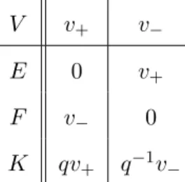
Following the representation theory of U(sl2), let V =hv+, v−i wherev+, v− are vectors of weights
+1,−1, respectively. The generators of Uq(sl2) act on V via
V v+ v−
E 0 v+
F v− 0
K qv+ q−1v−
Table 2.1: The fundamental Uq(sl2) representation The tensor product of V with itself decomposes into irreducible modules as
V ⊗V = Sym2qV ⊕C(q)
where
Sym2qV =hv+⊗v+, q−1v+⊗v−+v−⊗v+, v−⊗v−i
C(q)∼=
∧
2qV =hqv+⊗v−−v−⊗v+iwhere Sym2qV,
∧
2qV are quantum analogues of Sym2V and∧
2V, respecively. By Schur’s lemma, there exist module mapsp:V ⊗V →C(q) and i:C(q)→V ⊗V, unique up to a scalar. We give these explicitly byp:
v+⊗v+ 7→0 v+⊗v− 7→ −1
v−⊗v+ 7→q−1 v−⊗v− 7→0
2.3.2 FundRep(Uq(sp4))
The algebra Uq(sp4) has Cartan matrix
2 −2 −1 2
.
By Definition 2.2.7 above, this gives an explicit presentation of Uq(sp4). The sp4 weight lattice is spanned by weights1, 2, where (i, j) =δij. Type sp4 has roots±21,±2,±1±2. We have simple rootsα1 =1−2, α2 = 22. The fundamental weights are given byω1 =1,ω2 =1+2. The sum of positive roots is given byρ= 21+2. Finally, we write Γi,j for the irreducible Uq(sp4) representation of highest weight iω1+jω2.
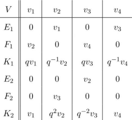
Denote V = Γ1,0 andW = Γ0,1. Letv1 be the highest weight vector ofV, and writev2 =F1v1, v3 =F2v2, and v4 =F1v1. Then the action ofUq(sp4) on V is given explicitly by
V v1 v2 v3 v4
E1 0 v1 0 v3
F1 v2 0 v4 0
K1 qv1 q−1v2 qv3 q−1v4
E2 0 0 v2 0
F2 0 v3 0 0
K2 v1 q2v2 q−2v3 v4
Table 2.2: The fundamental Uq(sp4) representation V As in the classical case, V ⊗V decomposes into irreducible representation
V ⊗V = Γ2,0⊕W ⊕C(q)
where Γ2,0 is aq-deformation of Sym2V.
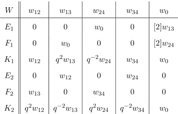
W w12 w13 w24 w34 w0
E1 0 0 w0 0 [2]w13
F1 0 w0 0 0 [2]w24
K1 w12 q2w13 q−2w24 w34 w0
E2 0 w12 0 w24 0
F2 w13 0 w34 0 0
K2 q2w12 q−2w13 q2w24 q−2w34 w0 Table 2.3: The fundamental Uq(sp4) representation W
The copy of the trivial representation in V ⊗V is spanned by the vector
z=q2v1⊗v4−q−2v4⊗v1−qv2⊗v3+q−1v3⊗v2.
Clearly,z has weight 0, and one may verify thatE1.z =E2.z = 0.
Finally, Γ2,0 can be seen to be 10 dimensional, having weight spaces ±2Li, ±Li±Lj and a 2-dimensional weight zero space, with weight vectors
(Weight±2Li) vi⊗vi for 1≤i≤6
(Weight±Li±Lj) q−1vi⊗vj +vj⊗vi for 1≤i < j ≤4 with i+j6= 5
(Weight 0)q−1v1⊗v4+qv4⊗v1+v2⊗v3+v3⊗v2
(Weight 0)q−1v2⊗v3+qv3⊗v2
Note that all the above explicitly gives the decomposition
V ⊗V = Γ2,0⊕W ⊕C(q).
the maps are given by
pC(q):
vi⊗vj 7→0 if i+j6= 5 v1⊗v4 7→ −q2
v2⊗v3 7→q v3⊗v2 7→ −q−1 v4⊗v1 7→q−2
and pW :
vi⊗vi 7→0
vi⊗vj 7→ −[2]wij ifi < j vj⊗vi7→q−1[2]wij ifi < j v1⊗v4 7→ −w0
v2⊗v3 7→ −qw0 v3⊗v2 7→q−1w0 v4⊗v1 7→w0.
We may then compute that
(pC(q))◦iC(q))(1) =pC(q) q2v1⊗v4−q−2v4⊗v1−qv2⊗v3+q−1v3⊗v2
=q2(−q2)−q−2(q2)−q(q) +q−1(−q−1) =−q−4−q−2−q2−q4
=−[2][6] [3]
so that (pC(q)⊗idV)◦(idV ⊗iC(q)) =idV. A similar computation shows that (idV ⊗pC(q))◦(iC(q)◦ idV) =idV.
2.3.3 FundRep(Uq(sp6))
The quantum group Uq(sp6) has Cartan matrix
2 −1 0
−1 2 −2
0 −1 2
.
By Definition 2.2.7 above, this gives an explicit presentation ofUq(sp6).
positive roots is given by ρ= 31+ 22+3. Recall that we write Γi,j,k for the irreducible Uq(sp6) representation of highest weight iω1+jω2+kω3.
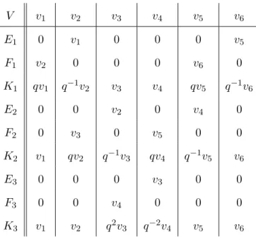
Denote the three fundamental representations byV = Γ1,0,0,W = Γ0,1,0, andX= Γ0,0,1. One can check that V is given by:
V v1 v2 v3 v4 v5 v6
E1 0 v1 0 0 0 v5
F1 v2 0 0 0 v6 0
K1 qv1 q−1v2 v3 v4 qv5 q−1v6
E2 0 0 v2 0 v4 0
F2 0 v3 0 v5 0 0
K2 v1 qv2 q−1v3 qv4 q−1v5 v6
E3 0 0 0 v3 0 0
F3 0 0 v4 0 0 0
K3 v1 v2 q2v3 q−2v4 v5 v6 Table 2.4: The fundamental Uq(sp6) representation V
We have the decomposition
V ⊗V = Γ2,0⊕W ⊕C(q)
where Γ2,0,0 is aq-deformation of Sym2V and we are slightly abusing notation and useV,W to denote Γ1,0,0 and Γ0,1,0, respectively.
The irreducible representation W has dimension 14:
(Weight±i±j) wij =qvi⊗vj−vj ⊗vi for 1≤i < j ≤6, i+j6= 7
(Weight 0)w0,1=v1⊗v6−v6⊗v1+qv2⊗v5−q−1v5⊗v2
(Weight 0)w0,2=v2⊗v5−v5⊗v2+qv3⊗v4−q−1v4⊗v3
Again, we haveC(q) as an irreducible summand of V ⊗V; it is spanned by
z=q3v1⊗v6−q−3v6⊗v1−q2v2⊗v5+q−2v5⊗v2+qv3⊗v4−q−1v4⊗v3.
The irreducible representation Γ2,0,0 is 21 dimensional, with one-dimensional weight spaces of
weight ±2Li,±Li±Lj, and a 3-dimensional weight zero space, with weight vectors:
(Weight±2Li) vi⊗vi for 1≤i≤6
(Weight±Li±Lj) q−1vi⊗vj +vj⊗vi for 1≤i < j ≤6 with i+j6= 7
(Weight 0)q−1v1⊗v6+qv6⊗v1+v2⊗v5+v5⊗v2
(Weight 0)q−1v2⊗v5+qv5⊗v2+v3⊗v4+v4⊗v3
(Weight 0)q−1v3⊗v4+qv4⊗v3
Now we have explicitly given the decomposition of V ⊗V = Γ2,0,0⊕W ⊕C(q) into irreducible representations.
Finally, the irreducible representation X = Γ0,0,1 also has dimension 14; consisting of single dimensional weight spaces of weights ±L1±L2±L3 and ±Li for i= 1,2,3. They are (viewing X⊂W ⊗V),
x1 =q−1w23⊗v1−w13⊗v2+qw12⊗v3
x2 =F3.w1 =q−1w24⊗v1−w14⊗v2+qw12⊗v4
x3 =F2.w2 =w0,2⊗v1−qw15⊗v2−w14⊗v3+q2w13⊗v4+qw12⊗v5
x4 =F1.w3 =w26⊗v1+q−1w0,2⊗v2−w0,1⊗v2−w24⊗v3+q2w23⊗v4+qw12⊗v6
x5 =F2.w4 =w36⊗v1+q−1w35⊗v2−w0,1⊗v3+q2w23⊗v5+qw13⊗v6
x6 =F1.w5 =q−1w36⊗v2−w26⊗v3+qw23⊗v6
x7 =F2.w3 =q−1w35⊗v1−w15⊗v3+qw13⊗v5
x9 =F1.w8 =w46⊗v1+q−1w45⊗v2−w0,1⊗v4+q2w24⊗v5+qw14⊗v6
x10=F2.w9 =w56⊗v1+q−1w45⊗v3−qw35⊗v4−w0,1⊗v5+qw0,2⊗v5+qw15⊗v6
x11=F1.w9 =q−1w46⊗v2−w26⊗v4+qw24⊗v6
x12=F2.w11=w56⊗v2+q−1w46⊗v3−qw36⊗v4−w26⊗v5+qw0,2⊗v6
x13=F2.w12=q−1v56⊗x3−v36⊗x5+qv35⊗x6
x14=F3.w13=q−1v56⊗x4−v46⊗x5+qv45⊗x6
As before, we define certain multiples of the projection and inclusion mapsiC(q) :C(q)→V ⊗V, iW :W → V ⊗V, pC(q) :V ⊗V → C(q), pW :V ⊗V → W. The inclusion maps iC(q), iW are defined above by writing howC(q), W sit inside ofV ⊗V. The mapspC(q),pW are defined by:
pC(q):
vi⊗vj 7→0 ifi+j6= 7 v1⊗v67→ −q3
v2⊗v57→q2 v3⊗v47→ −q v4⊗v37→q−1 v5⊗v27→ −q−2 v6⊗v17→q−3
and pW :
vi⊗vi7→0
vi⊗vj 7→ −[3]wij ifi+j 6= 7, i < j vj⊗vi 7→q−1[3]wij ifi+j6= 7, i < j v1⊗v67→ −[2]w0,1+w0,2
v2⊗v57→ −q2w0,1−q−1w0,2 v3⊗v47→qw0,1−q[2]w0,2 v4⊗v37→ −q−1w0,1+q−1[2]w0,2 v5⊗v27→q−2w0,1+qw0,2 v6⊗v17→[2]w0,1−w0,2
Using these maps, we compute
pC(q)◦iC(q)=pC(q)(q3v1⊗v6−q−3v6⊗v1−q2v2⊗v5+q−2v5⊗v2+qv3⊗v4−q−1v4⊗v3) =q3(−q−3)−q−3(q−3)−q2(q2) +q−2(−q−2) +q(−q)−q−1(q−1)
=−q−6−q−4−q−2−q2−q4−q6 =−[3][8]
and
(pW ◦iW)(w12) =pW(qv1⊗v2−v2⊗v1) =q(−[3]w12)−(q−1[3]w12) =−[2][3]w12
so that pC(q)◦iC(q) =−[3][8][4] idC(q) and pW ◦iW =idW.
Similar to the previous section, we compute that (pC(q)⊗idV) ◦(idV ⊗iC(q)) = idV and (idV ⊗pC(q))◦(iC(q)◦idV) =idV.
We may use these maps to define maps iC(q)→W⊗W :C(q)→W ⊗W andpW :W ⊗W →C(q). We make the definitions
iC(q)→W⊗W =− 1
[2][3](pW ⊗pW)◦(idV ⊗iC(q)⊗idV)◦(idV ⊗pC(q)⊗qV)◦(iC(q)⊗iC(q))
and
pW⊗W→C(q)=− 1
[2][3](pC(q)⊗pC(q))◦(idV ⊗iC(q)⊗idV)◦(idV ⊗pC(q)⊗idV)⊗(iW ⊗iW).
A computation3 then shows thatpW⊗W→C(q)◦iC(q)→W⊗W = [7][8]
[4] idC(q).
We also have maps iX :X→W ⊗V,jX :X→V ⊗W,pX :W ⊗V →X,qX :V ⊗W →X. The mapiX is defined by specifying howX sits insideW ⊗V; for example,
iX(x1) =q−1w23⊗v1−w13⊗v2+qw12⊗v3.
IncludingX ,→V ⊗W rather than X ⊂W ⊗V, the tensor factors are flipped and q is replaced by q−1. For example, in W ⊗V, the highest weight vectorx1 is instead given by
jX(x1) =qv1⊗w23−v2⊗w13+q−1v3⊗w12.
3
We definejX accordingly, by being the image of iX with tensor factors switched andq replaced by q−1.
The domains of pX, qX have dimension 6·14 = 84, so we do not record the image of every element of them here. Rather, we will find a much better way to record these maps, utilizing the
fact thatUq(sp4) is a subalgebra of Uq(sp6). However, for the sake of illustration, we do define the maps pX, qX on several elements:
pX :
w23⊗v1 7→ −q−1[3]x1 w13⊗v2 7→[3]x1 w12⊗v3 7→ −q[3]x1
and qX :
v1⊗w237→ −q[3]x1 v2⊗w137→[3]x1 v3⊗w127→ −q−1[3]x1
One can check thatpX, qX are−[3]2 times the projection maps. 2.4 Monoidal Categories
Next, let us discuss monoidal categories and their diagrammatic language. We follow the excellent
paper [31].
Definition 2.4.1. A category C is a class of objects ob(C) along with, for each pair of objects X, Y, a class HomC(X, Y) (we sometimes omit the subscript ifC is understood). The elements of
HomC(X, Y) are calledmorphisms (from X to Y). If f ∈HomC(X, Y), we also write f :X→Y.
Morphisms have the additional structure:
A function HomC(X, Y)×HomC(Y, Z)→HomC(X, Z) called composition; we write g◦f for
the image of (f, g).
For every object X, a morphism idX ∈ HomC(X, X) such that, for any morphism u ∈
Hom(X, Y) and any morphismv∈Hom(Z, X), we haveu◦idX =u and idX ◦v=v.
The composition of morphisms is associative (whenever defined).
A morphism f :A→B is anisomorphism if it has a two-sided inverse; i.e. there is a morphism g:B →Asuch that g◦f =idA and f◦g=idB.
Afunctor Ffrom a categoryC1toC2consists of a map sending each objectX∈ob(C1) to an object F(X)∈ob(C2) and, for all objects X, Y of C1, a set map F : HomC1(X, Y)→HomC2(F(X), F(Y))
F(idX) =idF(X).
F(f◦g) =F(f)◦F(g).
The functor F is called full if for any two objects x, y of C1, the induced map HomC1(X, Y) →
HomC2(F(X), F(Y)) is surjective; F is called faithful if for any two objectsx, y of C1, the induced
map HomC1(X, Y)→ HomC2(F(X), F(Y)) is injective. If F is full and faithful, we say F is fully
faithful. Finally,F is calledessentially surjective if each object of C2 is isomorphic to an object of the formF(x) for some objectx of CF1. The functorF is anequivalence of categories if it is fullly faithful and essentailly surjective.
Given categoriesC,D and functorsF, G:C → D, a natural transformation α:F ⇒G assigns to every objectX ∈ob(C) a morphismαX :F(X)→ G(X) such that for every f ∈HomC(X, Y),
we have that
F(X) F(Y)
G(X) G(Y)
F(f)
αX αY
G(f)
commutes. Finally, a natural isomorphism between functors F andGis a natural transformation from F toGwith a two-sided inverse.
Throughout this section, we will use the category of finite dimensional k-vector spaces as a
motivating example. The category Vectk has objects all finite dimensional k-vector spaces and
morphisms HomVectk(V, W) the collection of all linear transformations from V to W. Another example of a category is the category Set, which has objects sets and HomSet(X, Y) the set of all
functions fromX toY. There is a functorF : Vectk →Set, which, on objects, forgets about the vector space structure, and on morphisms, views a linear transformation as a function between sets.
Let us now discuss a diagrammatic formalism for categories. We depict an object by a label, and
a morphism from one object to another by drawing a strand between labels with a box containing a
morphism. We shall always read from bottom to top. For example, for objects A, B, we depict a morphism f :A→B by
A B
Composition is given by vertical stacking, and identity morphisms are shown as a strand with no
box. For example, given morphismsf :A→B and g:B →C, we drawg◦f as
A C
B f g
.
The fact that function composition is associative makes this notation (with three or more boxes)
well-defined. Further, note that the axioms that idB ◦f = f and f ◦idA = f translate to the diagrams
A B
f =
A B
f ,
B C g
=
B C g
respectively, which hold up to isotopy in the graphical language.
The category Vectk has more structure than we’ve described so far. For example, given two
objectsV, W of Vectk, there is another objectV⊗W of Vectk. Further, given morphismsS :V →X andT :W →Y, there is a corresponding morphismS⊗T :V ⊗W →X⊗Y. This is the structure we will formalize now.
Definition 2.4.2. A monoidal category is a category equipped with the following:
A functor ⊗:C × C → C
A (monoidal) unit I
For every pair of morphismsf :A→B and g:C→D, a morphismf ⊗g:A⊗C →B⊗D
A natural isomorphism λ:I⊗(−)→(−) with componentsλX :I⊗X →X
A natural isomorphism ρ: (−)⊗I →(−) with componentsρX :X⊗I →X
such that the diagrams commute:
The triangle identity:
(X⊗1)⊗Y X⊗(1⊗Y)
X⊗Y αX,1,Y
ρX⊗idY
idX⊗λY
The pentagon identity:
(W ⊗X)⊗(Y ⊗Z)
((W ⊗X)⊗Y)⊗Z W ⊗(X⊗(Y ⊗Z))
(W ⊗(X⊗Y))⊗Z W ⊗((X⊗Y)⊗Z) αW,X,Y⊗Z
αW⊗X,Y,Z
αW,X,Y⊗idZ
αW,X⊗Y,Z
idW⊗αX,Y,Z
Graphically, we depict the unit object I as an empty label (i.e., we draw nothing forI). The operation⊗ is given by horizontal juxtoposition. For example, we draw (the identity morphism of) A⊗B as
A B
.
We write a morphismh:A⊗B→C⊗D as
A C
B D
Iff :A→C and g:B→D are morphisms, their tensor product is drawn
A C f
B D
g .
Again, equalities between morphisms in a monoidal category correspond exactly to diagrams up to
isotopy. For example, for morphismsf :A→C and g:B →D, the identity
(idC⊗g)◦(f⊗idB) =f⊗g= (f ⊗idD)◦(idA⊗g)
corresponds to the isotopy
A C
f B D g
=
A C
f
B D
g =
A C f
B D
g
in the graphical language.
Returning to the example of Vectk, we actually have thatV ⊗W ∼=W ⊗V for all vector spaces V, W. This is the structure we shall formalize next.
is compatible with the associatiors, in the sense that the two diagrams
X⊗(Y ⊗Z)
(X⊗Y)⊗Z (Y ⊗Z)⊗X
(Y ⊗X)⊗Z Y ⊗(Z⊗X)
Y ⊗(X⊗Z)
βX,Y⊗Z
αX,Y,Z
βX,Y⊗idZ αY,Z,X
αY,X,Z idY⊗βX,Z
and
(X⊗Y)⊗Z
X⊗(Y ⊗Z) Z⊗(X⊗Y)
X⊗(Z⊗Y) (Z⊗X)⊗Y
(X⊗Z)⊗Y
βX⊗Y,Z
α−X,Y,Z1
idX⊗βY,Z α−Z,X,Y1
α−X,Z,Y1 βX,Z⊗idY
commute, called the hexagon relations.
Graphically, we write the isomorphism βA,B and its inverse as
βA,B =
B B
A A
, βA,B−1 = B
B
A A
In general, β◦β 6= id (if this equality does hold, we call the categorysymmetric. The fact that β−1◦β=id and β◦β 6=id are apparent in the graphical language:
The naturality of β says that for all morphisms f :A→B, we have
A f
C
C B
=
C A
C B
f ,
A f C
C B
=
C A
C B
f
One consequence of the naturality of β along with the hexagon relation is the Yang-Baxter equation
= .
In our example of Vectk the braidingβV,W is given by v⊗w7→w⊗v (and extending linearly). SinceβY,X◦βX,Y =idX⊗Y, we actually have that Vectk is symmetric. The categories of interest in this work, however, are not symmetric. Again, Vectk has more structure still; Given a vector
spaceV, there is a dual vector spaceV∗. The notion of dual objects is the next concept we wish to formalize.
Definition 2.4.4. An exact pairing between objectsAandB is a pair of morphismsη :I →B⊗A and :A⊗B →I such that the following triangles commute:
A A⊗B⊗A
A idA⊗η
idA
⊗idA ,
B B⊗A⊗B
B η⊗idB
idB
idB⊗
In this case, B is called theright dual of A andA is called theleft dual of B.
Finally, a category is called (left/right) autonomous if every objectA has a (left/right) dual object (denoted A∗ for right dual or∗Afor left dual).
A:A⊗A∗ →I, and 0A:∗A⊗A→I as follows:
ηA= A∗
I A
, ηA0 = A
I
∗A
, = A
I A∗
, 0 =
∗A
I A
.
The properties that the morphisms of the exact pairing must satisfy are then the “snake relations”
= , =
if the category is right autonomous, and
= , =
if the category is left autonomous.
Given a morphism f : A→ B, may define new morphisms f∗ :B∗ → A∗ and ∗f : ∗B → ∗A,
called the adjoint mates of f as
f∗=
A B
f
B∗ A∗
, ∗f =
A B
f
∗B
∗A
.
In the case of an autonomous category which is also braided, we have the following.
Lemma 2.4.5. A braided monoidal category is autonomous if and only if it is right autonomous.
Returning to our example, we see that Vectk is autonomous. An object V has dual V∗ = Hom(V,k), and the pairings are defined byA(v⊗f) =f(v) andηA: 17→
P
v∗i ⊗vi where{vi}is a basis ofV. The maps0A andηA0 are similar. Checking the snake relations are then straightforward. Given a morphism T :V → W, the adjoint mate T∗ : W∗ → V∗ is given by T∗(f) = f◦T. In the case of Vectk, there is a natural isomorphism between a vector space V and (V∗)∗ (given by v7→(f 7→f(v))). This is the next concept we would like to formalize.
Definition 2.4.6. A pivotal category is a (right) autonomous category along with a monoidal natural isomorphismiA:A→(A∗)∗ such that
A∗ A∗∗∗
A∗ iA∗
idA∗ i∗ A
commutes.
A pivotal category is always autonomous (right duals are immediately also left duals). The
assumption that iA is a monoidal natural transformation means that iI is cannonoical and the following commutes:
A⊗B
A∗∗⊗B∗∗ (A⊗B)∗∗
iA⊗iB
iA⊗B
∼
=
The diagrammatics for a pivotal category are the same as for an autonomous category, but we
have more freedom in the types of diagrams we can draw. For example, if h :A∗⊗A∗ → I is a morphism, we have the following equalities:
h = h = h
In a braided autonomous category, there is a natural isomorphism bA:A∗∗→Agiven by
bA= A
A∗∗
A∗
with inverse
b−A1=
A∗∗
A
A∗ .
Sinceb is not a monoidal natural transformation, this need not define a pivotal structure. However, in one special case, it does. First, a definition.
Definition 2.4.7. A twist on a braided monoidal category is a natural family of isomorphisms θA:A→A such thatθI =idI and, for allA, B,
A⊗B B⊗A
A⊗B B⊗A
βA,B
θA⊗B θB⊗θA
βB,A
commutes. If a braided monoidal category has a twist, we say it is abalanced monoidal category.
We then have the connection, a proof of which may be found in [31].
Lemma 2.4.8. Given a braided autonomous categoryC, if there is a twistθ, theniA=b−A1◦θA defines a pivotal structure. Conversely, given a pivotal structurei, then θA=bA◦iAdefines a twist.
Finally, a pivotal braided category (or balanced and autonomous) is said to be ribbon (ortortile)
1.
= .
2. θA∗ = (θA)∗
When graphically describing a ribbon category, we may replace the strands with ribbons. The
twist map is then depicted as a twist as below in [31].
Figure 2.1: The twist mapθAin a ribbon category
If an objectA is isomorphic to A∗, a coherent self-duality is an isomorphismhA:A→A∗ such that the diagram
A∗ (A∗)∗
A∗ iA∗
θA∗
h∗A
commutes.
We are now prepared to more precisely state the connection between link invariants and quantum
groups. The following theorem is due to Reshetikhin-Turaev in [26].
Theorem 2.4.9. Forg semisimple,Rep(Uq(g)) is a ribbon category.
Thus, given a link diagram LD, we may label each component of L by an irreducible Uq(g)
representation, and interpret the link diagram as an endomorphism of the trivial representation;
that is, as an element ofC(q).
For example, earlier we saw the diagram of an oriented Hopf link
If we color each of the components by an irreducible Uq(g) representation, the diagram (which we have drawn slightly differently)
V W
may be interpreted as the morphism
0V ◦(idV∗⊗V ⊗W)◦(idV∗⊗βW,V ⊗idW∗)◦(idV∗⊗βV,W ⊗idW∗)◦(ηV ⊗idW⊗W∗)◦η∗
W
from C(q) to itself; thus, as an element of C(q).
2.5 Temperly-Lieb
In this section, we discuss the Temperly-Lieb category, which is the prototypical diagrammatic
presentation of a category of representations. We start with the more familiar Temperly-Lieb
algebra.
Definition 2.5.1. We define theTemperly-Lieb algebra on n strands (n > 0). Let TLn be the
C(q)-algebra generated by 1, e1, . . . , en−1 modulo relations:
eiej =ejei if|i−j|>1
eiei±1ei =ei
e2i =−[2]ei.
We claim TLn admits a diagrammatic presentation. Take the square I×I, and markn points (calledboundary points) onI× {0}and onI× {1}. Define acrossinglessn, ntangle to be an isotopy class of smoothly embedded disjoint 1-manifolds, those with boundary having boundary points
exactly the marked points of the marked square.
For example, when n= 3,
, ,
crossingless n, ntangles modulo the relation
=−[2].
Endow Tn with the structure of an algebra by stacking and re-scaling in the y-direction. For example,
!
× + [2]
!
= + [2] = −[2]2
Theorem 2.5.2. The algebra Tn is a diagrammatic presentation of TLn.
Proof. Define a map φ:TLn→Tn by
17→
1 . . .
n
, ei 7→
1 . . .
i i+ 1 i i+ 1
. . .
n
.
First, we claim thatφis surjective. We only give the idea here; a full proof is in [35]. First, given a crossingless tangle, apply an isotopy to write it in terms only of vertical segments and semicircles
(with horizontal diameter). This is possible by an argument involving the number of turns an arc
makes when it connects marked points on the same side or opposite side. Finally, arcs on opposite
sides until the crossingless tangle is in the desired form. As an easy example, consider
= =φ(e2e1).
Let’s verify that φis injective. First, if |i−j|>1, we have thatφ(eiej) =φ(ejei) by isotopy. We also have
φ(eiei+1ei) =
i
=
i
where we have omitted drawing the other strands. Similarly,φ(eiei−1ei) =φ(ei). Finally,
φ(e2i) =
i
−[2]
i
soφis injective.
In fact, we can “upgrade” the Temperly-Lieb algebra to a category. Define the Temperly-Lieb
category TL to be theC(q)-linear monoidal category with objects Z≥0 and Hom(m, n) the set of formal C(q)-linear combination of crossingless m, n tangles (an isotopy class of smoothly embedded disjoint copies ofI with boundary points on m marked points onI× {0}and nmarked points on I× {1}) modulo the relation
=−[2].
The monoidal structure on objects is defined by m⊗n=m+nand on morphisms by horizontal concatenation (and re-scaling in thex-direction). Morphism composition (when defined) is given by vertical concatenation (and re-scaling in the y-direction). For each n > 0, note thatTLn = EndTL(n).
Theorem 2.5.3. There is a fully faithful, essentially surjective monoidal functor Ψ : T L → FundRep(Uq(sl2)).
Proof. The functor Ψ, on objects, sends n7→V⊗n, and on morphisms, sends
7→p , 7→i
where these are the projection and inclusion maps defined earlier.
It is straightforward to check that this map factors through the TL relations. By some Cerf and Morse theory, the only isotopy relations needed to be checked are the “snake” relations
so we must check that (p⊗idV)◦(idV ⊗i) =idV and (idV ⊗p)◦(i◦idV) =idV. Indeed,
(p⊗idV)◦(idV ⊗i)(v+) =qv+⊗v+⊗v−−v+⊗v−⊗v+= 0−(−1)v+=v+
(by Schur’s lemma, the snake relation holds up to a scalar, so we only need to verify it on one
element). Similarly, one can check that (idV ⊗p)◦(i⊗idV) =idV. Finally, we must check that p◦i=−[2]1k. Indeed,
(p◦i)(z) =p(qv+⊗v−−v−⊗v+) =−q−q−1 =−[2].
Thus, Ψ factors through the relations of TL.
Remark 2.5.4. The functor Ψ above is also essentially surjective, full, faithful, and braided. Proofs of these can be found in [29] [17].
Remark 2.5.5. Another way to describe TL is as the pivotal category freely generated by one self-dual object modulo the local relation
=−[2].
By “freely generated,” we mean that we allow all finite tensor products of the object, and all
compositions of tensor products of the identity and unit/counit morphisms.
By “self-dual,” we mean that there is a coherent self-duality from this object to its dual.
By “local relation,” we mean modulo the ideal generated (by allowing all tensor products and
all compositions) of the relation.
After extending scalars to C(q−1/2, q1/2), the braiding onTL is given by
=q1/2 +q−1/2 .
In fact, this gives the Jones polynomial, as defined in Section 2.1. As before, the fractional powers
2.6 Web categories
In pioneering work [17], Kuperberg extended the Temperley-Lieb description ofRep(Uq(sl2)) to Uq(g) for rank two simpleg,sl2,sp4, andg2. We first highlight the caseg=sp4, as it is the most relevant to our present work.
The type C2 spider, denoted here by Web(sp4), is a combinatorial description of the category Rep(Uq(sp4)). Explicitly, Web(sp4) is obtained from the C(q)-linear ribbon category pivotally generated by self-dual objects{1,2} and the morphism
1 1 2
∈HomWeb(sp4)(1⊗1,2)
with local relations:
=−[2][6]
[3] , =
[5][6]
[2][3] , = 0 , =−[2] 2
− = − , = 0.
Following [17], we refer to these graphs aswebs. Throughout, we’ll follow the conventions that we
won’t label the (co)domain in our morphisms, electing instead to color our web edges. Throughout,
blackdenotes 1-labeled edges and blue denotes 2-labeled edges. Further, as can be inferred from the above, we read all webs as mapping from bottom to top.
Kuperberg then proves the following result.
Theorem 2.6.1. There is an equivalence of monoidal categoriesWeb(sp4)∼=FundRep(Uq(sp4)). In fact, Kuperberg proves analogues of this result for all rank 2 Lie algebras (i.e. additionally
forsl3 andg2), and extends this result to an equivalence of ribbon categories by giving explicitly
formulae for the braidings in the web categories.
For the sake of completeness, we include Kuperberg’s other web categories here.
TheWeb(sl3) category is the k-linear ribbon category pivotally generated by objects{+,−}. These objects are not self-dual; rather, the duality structure is given by reversing the order and
category Web(sl3) has morphisms generated by trivalent vertices
+ +
−
∈HomWeb(sl3)(+⊗+,−) ,
− −
+
∈HomWeb(sl3)(− ⊗ −,+)
modulo the local relations
= [3] , = [2] , = + .
Finally, the categoryWeb(g2) is the k-linear ribbon category pivotally generated by self-dual objects{1,2}and morphisms
1 1 1
∈HomWeb(g2)(1⊗1,1) ,
1 1 2
∈HomWeb(g2)(1⊗1,2)
modulo the relations
= [2][7][12]
[4][6] , =
[7][8][15]
[3][4][5] , = 0 , =− [3][8]
[4]
= [6]
[2] , = [3]
+
−[4]
[2] +
= − [4][6]
[2][12] + 1
[3] −
= 4
X
i=0 ρ2πi/5
− 4
X
i=0 ρ2πi/5
where in the last equation above, ρθ rotates the picture by an angle of θ(so we have 10 total terms in the last equation).
It remained an open problem for over ten years to extend Kuperberg’s results beyond rank two,
despite progress in the PhD theses of Kim [15] and Morrison [19]. In [4], breakthrough work of
Again, for the sake of completeness, we include the definition of the general sln web category.
The typeAn−1 spider, denotedWeb(sln), is pivotally generated by the 2n−2 objects{1,1∗, . . . , n− 1,(n−1)∗} and morphisms
a b a+b
,
a∗ b∗ (a+b)∗
, a
a∗
, a∗
a
Generally we will omit the ∗label from an object and instead look at the orientation of the edge. We quotient by the relations:
k n−k
= (−1)k(n−k)
k n−k
,
a+b
b a
a+b =
a+b a
a+b ,
a
a+b b
a
=
n−a b
a+b
= , = , =
a b
=
a+b a
a+b
,
m a
n b
=X i
m−n+b−a i
n b−i
m a−i
CHAPTER 3
Ψ :Web(sp6)→FundRep(Uq(sp6)) is well-defined
First, we recall the definition of Web(sp6)
Definition 3.0.1. The categoryWeb(sp6) is the (strictly pivotal) C(q)-linear category generated by the self-dual objects{1,2,3} and with morphisms generated by
1 1 2
∈HomWeb(sp6)(1⊗1,2) ,
1 2
3
∈HomWeb(sp6)(1⊗2,3)
modulo the relations:
=−[3][8]
[4] , = 0 , =−[2][3] , =−[3]
2 , =
= 0 , = [3]2 + 1
[2] −[3]
− = [2]
−
, − = [2] −
!
Remark 3.0.2. We record the following useful consequences of the above:
= [7][8]
[4] , =−
[6][7][8] [2][3][4]
= 0 = , = [2][7] , =−[6][7]
[2] , = [3][6]
[2]
=−[4] , =−[3][4]
[2] , =
[3]
[2] .
In this section, we prove that Ψ :Web(sp6)→FundRep(Uq(sp6)) is well-defined. The functor Ψ is defined on objects by sending an edge labelled by ito the irreducible Uq(sp6) representation of highest weightωi, and on morphisms, sending trivalent vertecies to the maps ofUq(sp6) modules. Remark 3.0.4. There is a standard choice of ribbon element forUq(g), which acts on an irreducible representation with highest weight λ byKρ (i.e. q−(λ,λ+2ρ)), where ρ is the half-sum of positive roots. However, following [32] and [34], we use a non-standardribbon element, which instead acts by−Kρ (i.e. −q−(λ,λ+2ρ)) on irreducible representations in an odd tensor product of V, and Kρ q−(λ,λ+2ρ) on irreducible representations in an even rtensor product ofV (this is well-defined due to the plethysm of type C).
One strategy is to present Web(sp6) by generators and relationsas a monoidal category, define the functor on the generating morphisms, and then check the requisite relations. This quickly
becomes computationally intensive. We instead proceed via an indirect proof which is more
conceptual. The proof strategy will involve computing the dimension of various Hom spaces in
FundRep(Uq(sp6)) to argue that there must be a relation between certain webs; we then compose these relations with other webs which allow us to evaluate the webs, giving a necessary condition
for the coefficients of the relation. We eventually find enough necessary conditions to solve for the
coefficients. A similar proof strategy was used by Kuperberg in [16] to find relations in theg2 spider,
and in the Ph.D. thesis of Kim [15] to find relations in thesl4 spider.
Theorem 3.0.5. There exists an essentially surjective functor Ψ :Web(sp6)→FundRep(Uq(sp6)).
Proof. First, we recall from the background. We haveV ⊗V = Γ2,0,0⊕W ⊕C(q) andV ⊗W = Γ1,1,0⊕X⊕V. Both of these imply that Homsp6(V⊗V, W) and Homsp6(V⊗W, U) are 1-dimensional, by Schur’s Lemma. Choosing a non-zero morphism in each of these Hom-spaces, there exists a
pivotal functor Ψ from the strict pivotal category freely generated by self-dual objects{1,2,3} and the morphisms
1 1 2
and
1 2
3
It remains to show that Ψ descends to the quotient obtained by imposing the relations in
Web(sp6). First, note that
Ψ
= 0 and Ψ
= 0 (3.0.1)
since Homsp6(W,C(q)) = 0 and Homsp6(X⊗X, W) = 0. Further
Ψ
=δ·Ψ
for someδ∈C(q) since Homsp6(W, W)
∼
=C(q). We recall the quantum dimensions of V,W,X:
dimq(V) =[3][8]
[4] , dimq(W) = [7][8]
[4] , dimq(X) =
[6][7][8] [2][3][4]
By our choice of ribbon element (Remark 3.0.4) which acts by−Kρ onV andX, butKρ onW, we have
Ψ
=−[3][8] [4] , Ψ
= [7][8] [4] , Ψ
=−[6][7][8]
[2][3][4]. (3.0.2) Because Homsp6(W, W) is 1-dimensional by Schur’s Lemma, we have a relation of the form
Ψ
=ωΨ
“Closing” this relation gives
Ψ
!
=ωΨ
so that δ[7][8][4] =ω
−[3][8][4] ; thus,
Ψ
=−δ[7] [3] Ψ
. (3.0.3)
Next, the tensor product decomposition
implies that the images under Ψ of
, , (3.0.4)
are linearly independent, hence give a basis for EndUq(sp6)(V ⊗V). Thus, we must have a relation
of the form
Ψ
+γ·Ψ
=α·Ψ
+β·Ψ
For someα, β, γ∈C(q). Applying this relation twice, we see
γ2·Ψ
=−γ ·Ψ
+αγ·Ψ
+βγ·Ψ
= Ψ
−α·Ψ
−β·Ψ
+αγ·Ψ
+βγ·Ψ
= Ψ
+ (αγ−β)·Ψ
+ (βγ−α)·Ψ
.
By linear independence, we must have that γ2 = 1 and β=γα. Thus,
Ψ
+γ·Ψ
=α·
Ψ
+γ·Ψ
. (3.0.5)
Closing the 1-labelled edges on the right side, we have
Ψ +γ·Ψ
=α·
Ψ
+γ·Ψ
.
Applying Equations (3.0.1), (3.0.3), (3.0.2), we see that
−γδ[7] [3] =α
−[3][8] [4] +γ
so, recalling that [3][8][4] = [7]−1 and γ2 = 1,
δ[7] = [3]α(γ([7]−1)−1). (3.0.6)
Next, becauseFundRep(Uq(sp6)) inherits a braidingβ fromRep(Uq(sp6)), it follows that
βV,V =κ·Ψ
+λ·Ψ
+µ·Ψ
for someκ, λ, µ∈C(q). The self-duality structure then implies that
βV,V−1 =κ·Ψ
+λ·Ψ
+µ·Ψ = (κ+µαγ)·Ψ
+ (λ+µα)·Ψ
−µγ·Ψ
where in the second line, we have applied Equation (3.0.6).
Expanding βV,V−1 βV,V gives
βV,V−1 βV,V =κ(λ+µα)·Ψ
+
λ(λ+µα) +κ(κ+µαγ) +λ(κ+µαγ)
−[3][8] [4]
·Ψ
+ −µγκ+µ(λ+µα)−δµ2γ·Ψ
The equality βV,V−1 βV,V = idV⊗V, together with linear independence of the images of (3.0.4), implies that
κ(λ+µα) = 1 κ
λ+
λ+µα κ+µαγ =
[3][8] [4]
λ+µα=γ(κ+µδ).
(3.0.7)
Substituting the left-hand side of the third into the first, we have
κγ(κ+µδ) = 1. (3.0.8)
Recall, as in Remark 3.0.4, that we are using the conventions in [32], the ribbon element acts on
a representation of highest weightλvia q−(λ,λ+2ρ), and that we have chosen the ribbon element to act via thenegative full twist, so the ribbon element acts onV via −q−(ω1,ω1+2ρ); thus,
Ψ
!
=−q−7·Ψ
!
and Ψ
!
=−q7·Ψ
!
Setting
we have that
=κ +λ +µ =κ +[3][8] [4]
so that
κ−λ([7]−1)
idV = Ψ
!
=ν|VidV =−q−(ω1,ω1+2ρ)idV =−q−7idV.
Thus
λ= κ+q
−7
[7]−1 (3.0.9)
Similarly, the ribbon element acts onW via q−(ω1+ω2,ω1+ω2+ρ)=q−12, so
Ψ
!
=q−12·Ψ
!
and Ψ
!
=q12·Ψ
!
First, note that
=κ +λ +µ = (κ+δµ)
So that
= 1 δ
= 1 δ
=−q 7 δ
=−q 7 δ