Chapter 18
E
ff
ect modification and interactions
18.1
Modeling e
ff
ect modification
4
0
5
0
6
0
7
0
8
0
9
0
1
0
0
w
e
ig
h
t
30 40 50 70
dose
male female
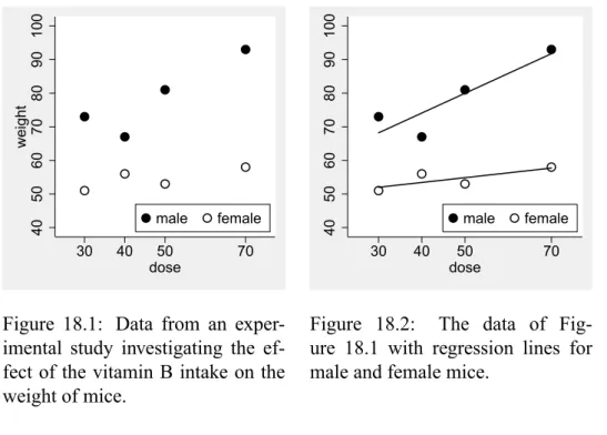
Figure 18.1: Data from an exper-imental study investigating the ef-fect of the vitamin B intake on the weight of mice.
4
0
5
0
6
0
7
0
8
0
9
0
1
0
0
30 40 50 70
dose
male female
Figure 18.2: The data of Fig-ure 18.1 with regression lines for male and female mice.
In some applications one is interested in the question how one covariate may affect the effect of another covariate. Figure 18.1 illustrates a typical situation of this type, in which the effect of the vitamin B intake on the weight of mice seems to differ between male and female mice. If we fit regression lines separately for male and female mice (Figure 18.2), it looks like that the vitamin B has only a small effect in female mice, but a large effect in male mice.
Fitting two regression lines, however, does not directly allow to compare the two lines in the sense of assessing the statistical significance of the difference between the two lines. This can
be approached by considering a joint model across the two groups. Introducing the random variables
X1= Vitamin B intake (in mg) and
X2 = (
1 if mouse is male 0 if mouse is female we can describe the situation by two separate regression models:
µ(x1,x2)= (
βA0 +βA1x1 ifx2 =1 βB0 +βB1x1 ifx2 =0
(∗)
withβA1 denoting the slope in male mice andβB1 denoting the slope in female mice as the main parameter of interest. However, this description does not have the usual form of a regression model still. This can be approached by regarding X1 as actually two different covariates, one defined in the male and one defined in the female mice:
X1A =
(
X1 if x2= 1 0 if x2= 0
X1B =
(
0 if x2= 1
X1 if x2= 0
We can now consider a regression model with the covariatesX1A,X1B andX2 which reads ˜
µ(x1A,xB1,x2)= β˜0+β˜A1x A
1 +β˜
B
1x
B
1 +β˜2x2 .
Here ˜βA1 denotes the effect of changing X1 in the male mice, and ˜β1B describes the effect of changingX1in the female mice, and hence it is not surprising that ˜βA1 =β1Aand ˜βB1 =βB1. Indeed, this model is equivalent to the “double” model (*) with the relations
˜
β0= βA0, β˜ A
1 = β
A
1, β˜
B
1 =β
B
1, and ˜β2 =β0B−β A 0 because in the casex2 =0 we have
µ(x1,0)=β0A+β A
1x1 and ˜µ(x1A,0,0)=β˜0+β˜1Ax A
1 =β˜0+β˜A1x1
and in the casex2 =1 we have µ(x1,1)=β0B+β
B
1x1 and ˜µ(0,xB1,1)= β˜0+β˜1Bx B
1 +β˜2 =β˜0+β˜2+β˜B1x1
Consequently, if fitting a regression model with the three covariates XA
1, X
B
1 andX2 to the data of Figure 18.1, we obtain an output like
variable beta SE 95%CI p-value
intercept 47.714 7.845 [25.933,69.495] 0.004
dosemale 0.589 0.158 [0.151,1.026] 0.020
dosefemale 0.143 0.158 [-0.295,0.581] 0.416
18.1. MODELING EFFECT MODIFICATION 249
and we obtain ˆβA1 =0.589 and ˆβB1 =0.143 as the slope parameter estimates in males and females, respectively. To assess the degree of effect modification, we will look at the difference between the slopes, i.e.
γ= βB1 −βA1
and we obtain ˆγ = βˆ1B − βˆA1 = 0.589 − 0.143 = 0.446. By further steps we can obtain a confidence interval of [−0.173,1.065] and a p-value of 0.116. So the evidence we have in favor for a true difference between male and female mice with respect to the effect of vitamin B intake is limited. However, the large confidence interval suggests that the difference may be substantial. Note that it does not make great sense to look at the p-values of ˆβB1 and ˆβA1, since it is not the aim of our analysis to assess the question, whether there is an effect in each subgroup, but to assess whether there is a difference in the effect.
−1
−.
5
0
.5
1
lo
g
it
(re
l.
f
re
q
u
e
n
cy)
female male
placebo treatment
female male
placebo treatment placebo treatment
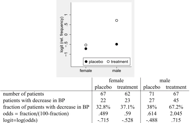
number of patients 67 62 71 67
patients with decrease in BP 22 23 27 45
fraction of patients with decrease in BP 32.8% 37.1% 38% 67.2%
odds=fraction/(100-fraction) .489 .59 .614 2.045
logit=log(odds) -.715 -.528 -.488 .715
Figure 18.3: Data from a clinical trial on an antihypertensive treatment and a visualisation of this data
Figure 18.3 illustrates a second example in which the effect of an antihypertensive treatment is considered to be dependent on sex. We can see that in females the treatment difference can be expressed as an empirical odds ratio of 1.207 = 0.5900.489, whereas in the males we obtain an odds ratio of 3.331= 2.0450.614, i.e. the treatment effect is much bigger in males, as we can also see in the graph of Figure 18.3. We can now use logistic regression to obtain a confidence interval and a p-value for the ratio between these two odds ratios, which describes to which degree sex alters the treatment effect. Introducing the two covariates
X1 = (
1 if treatment is given to the patient 0 if placebo is given to the patient
and
X2 = (
1 if patient is male 0 if patient is female we can describe the situation again by a double regression model
logitπ(x1,x2)= (
β0A+βA1 if x2= 1 β0B+βB1 if x2= 0
and eβA1 is identical with the odds ratio in males, and eβB1 is identical with the odds ratio in females. Consequently,eγ forγ= βB
1 −β
A
1 satisfies
eγ =eβ1B−β
A
1 = e
βB1
eβA
1
i.e. it is the ratio of the odds ratio in males and females.
As above it is equivalent to consider a regression model in the three covariatesXA
1, X
B
1 andX2
and in fitting this model we obtain an output like
variable beta SE 95%CI p-value
intercept -0.716 0.260 [-1.226,-0.206] 0.006
treatmale 1.204 0.357 [0.504,1.904] 0.001
treatfemale 0.188 0.370 [-0.537,0.912] 0.612
sex 0.227 0.357 [-0.472,0.927] 0.524
The difference ˆγ = βˆB1 −βˆA1 = 1.204−0.188 = 1.016 corresponds to the difference we see in Figure 18.3, and by further steps we can obtain a confidence interval of [0.009,2.024]. By expo-nentiating the estimate and the confidence interval we obtain 2.763 with a confidence interval of [1.009,7.568]. Note that 2.763 is exactly the ratio between the two empirical odds ratios 3.331 and 1.207 we have computed above.
The considerations above can be easily extended to categorical covariates. If, for example, a categorical covariate X2 with three categories A, B, and C modifies the effect of another covariateX1, we have just to construct for each category a covariate:
X1A =
(
X1 ifx2 =A 0 ifx2 ,A
X1B =
(
X1 ifx2 =B 0 ifx2 ,B
X1C =
(
X1 ifx2 =C 0 ifx2 ,C
18.1. MODELING EFFECT MODIFICATION 251
1
0
2
0
3
0
4
0
5
0
6
0
re
la
ti
ve
f
re
q
u
e
n
cy
30−39 40−49 50−59 60−69 70−79
age classes
non smokers smokers
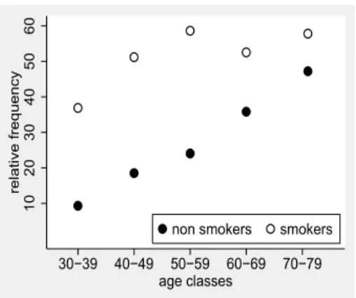
Figure 18.4: The relative frequency of hypertension in dependence on the smoking status and age in an observational study with 1332 subjects. Age is available in years and only grouped into categories for this graph.
It remains to consider the case, in which we are interested in modeling the modifying effect of a continuous covariate on the effect of another covariate. Figure 18.4 illustrates such a situation with the two covariates
X1 = (
1 subject is a smoker 0 subject is no smoker and
X2 = age of subject (in years) , and we are interested in how age changes the effect of smoking.
Since X2 is a continuous covariate, we cannot apply the approach defining a version of X1 for any value ofX2. Instead, we have to consider directly the model we are interested in, i.e. a model allowing the effect of X1to depend onX2. We can write such a model as
logitπ(x1,x2)= β0+β1(x2)x1+β2x2 ,
i.e. we allow the regression coefficient of X1 to depend on the value of X2. The most simple type of dependence is a linear relation, i.e. we specify the dependence as
β1(x2)=α0+α1x2
such thatα0is the effect ofX1 if x2 = 0 andα1describes the increase of the effect ofX1 if we increaseX2by 1.0. If we now insert this in the model above, we obtain
logitπ(x1,x2)=β0+(α0+α1x2)x1+β2x2 , which we can rewrite as
logitπ(x1,x2)= β0+α0x1+α1x1x2+β2x2 . (∗∗) This is a model we can fit directly to our data. We have just to introduce a new covariate
and we fit a linear model in the three covariates X1, X2 and X3. If we do this for the data of Figure 18.4, we obtain an output like
variable beta SE 95%CI p-value
intercept -3.906 0.385 [-4.660,-3.152] <0.001
smoking 2.955 0.506 [1.963,3.947] <0.001
age 0.051 0.006 [0.039,0.064] <0.001
agesmoking -0.033 0.009 [-0.050,-0.016] <0.001
So we obtain the estimate ˆα1 =−0.033, suggesting the the difference between smokers and non smokers with respect to the probability of hypertension (on the logit scale) decreases by 0.033 with each year of age, or by 0.33 with 10 years of age. Or, if one prefers to use odds ratios, that the odds ratio comparing smokers and non smokers decreases by a factor ofe−0.33 = 0.72 with ten years of age.
However, just presenting this result would be a rather incomplete analysis, as we only know, that the difference becomes smaller, but we do not know, how big the effect of smoking is at different ages. Hence it is wise to add estimates of the effect of smoking at different ages, e.g. at the ages of 35 and 75. The effect of smoking at a certain age x2 is, as mentioned above, α0 +α1x2. According to (**),α0 is just the coefficient of X1 in the fitted model, i.e. from the output above we obtain ˆα0 =2.955. So we obtain estimates for the effect of smoking at the age of 35 as
ˆ
α0+αˆ1×35= 2.955+(−0.033)×35= 1.812 or an OR ofe1.812= 6.12 and at the age of 75 we obtain
ˆ
α0+αˆ1×75= 2.955+(−0.033)×75=0.506 or an OR ofe0.506= 1.66 .
So the odds ratio for the effect of smoking on hypertension is at the age of 75 only about a fourth of the odds ratio at the age of 35.
Remark:Note that the computation of the effect of smoking at selected ages contributes also to assessing the relevance of the effect modification. In our example, we observe a reduction of the effect of smoking (on the logit scale) from 1.812 at age 35 down to 0.506 at the age of 75. So over the whole range we have a substantial effect of smoking. However, the same estimate of ˆα1 will also appear, if the effect of smoking decreases from 0.612 down to −0.694. In this case the effect of smoking vanishes with increasing age and has at the end the opposite sign. Such a qualitative change is much more curios and typically much more relevant than the purely quantitative change seen above.
18.2
Adjusted e
ff
ect modifications
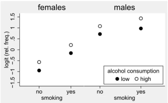
The adequate assessment of effect modifications may require to take other covariates into ac-count. As an example, let us consider the data shown in Figure 18.5. The effect of alcohol
18.2. ADJUSTED EFFECT MODIFICATIONS 253
−1
.5
−1
−.
5
0
.5
1
1
.5
lo
g
it
(re
l.
f
re
q
.)
no yes
smoking females
no yes
smoking
low high
alcohol consumption males
Figure 18.5: The relative frequency of hypertension (on the logit scale) in dependence on smok-ing status, alcohol consumption and sex.
−1
.5
−1
−.
5
0
.5
1
1
.5
lo
g
it
(re
l.
f
re
q
.)
no yes
smoking
low high
alcohol consumption
Figure 18.6: The relative frequency of hypertension (on the logit scale) in dependence on smok-ing status and alcohol consumption.
consumption seems to be roughly identical in all four subgroups defined by smoking status and sex. However, if we ignore in our analysis the variable sex (Figure 18.6), it looks like that the effect of alcohol consumption is bigger in smoking subjects. Indeed, if we fit a logistic model to the data of Figure 18.6 allowing different effects of alcohol for smokers and non smokers, we obtain an output like
variable beta SE 95%CI p-value
alcoholsmoker 0.801 0.218 [0.374,1.229] <0.001
alcoholnosmoker 0.385 0.230 [-0.067,0.836] 0.095
smoking 0.509 0.233 [0.052,0.965] 0.029
suggesting different effects of alcohol consumption for smokers and non smokers. However, if we adjust the analysis for sex, we obtain an output like
variable beta SE 95%CI p-value
alcoholsmoker 0.374 0.235 [-0.086,0.833] 0.111
alcoholnosmoker 0.418 0.244 [-0.061,0.896] 0.087
smoking 0.583 0.247 [0.100,1.067] 0.018
sex 1.390 0.172 [1.053,1.726] <0.001
with nearly identical effects of alcohol consumption for smokers and non smokers, as suggested by Figure 18.5. The explanation for this striking difference can be found in Figure 18.7, in which we have added the number of subjects in each subgroup. We can see that the subgroup of smokers with high alcohol consumption is dominated by males, whereas in all other subgroups the majority of subjects are females. And as males have in this study a higher risk for hyperten-sion than females, this contributes to the high frequency of hypertenhyperten-sion in smokers with high alcohol consumption resulting in the pattern we have seen in Figure 18.6.
Hence this examples illustrates that it is important to adjust for potential confounders in the analysis of effect modifications also.
86
91 91
65
−1
.5
−1
−.
5
0
.5
1
1
.5
lo
g
it
(re
l.
f
re
q
.)
no yes smoking females
61
62 67
187
no yes
smoking low high alcohol consumption
males
Figure 18.7: The relative frequency of hypertension (on the logit scale) in dependence on smok-ing status, alcohol consumption and sex. The numbers indicate the number of subjects behind the relative frequency.
18.3
Interactions
Whenever one starts to model an effect modification one has to be aware of a slight arbitrariness, because we decide in advance that X1 modifies the effect of X2, and not vice versa. However, these two perspectives are equivalent and – in principle – indistinguishable. Let us consider for example Figure 18.4. We have used it to illustrate how age modifies the effect of smoking, but we can also regard it as an illustration that the effect of age is different for smokers and non smokers: The frequency of hypertension increases with age slower for smokers than for non smokers. Similar in Figure 18.3 we may say that each treatment is associated with a sex
18.3. INTERACTIONS 255
effect of its own instead of that sex alters the treatment effect. It may happen that one of the two perspectives sounds more logically but in principle both perspectives are correct.
The symmetry of both perspectives can be also nicely illustrated by our considerations above in the case of continuous covariates. We have shown that modeling the modifying effect ofX2 on the effect ofX1leads to the expression
β0+(α0+α1x2)x1+β2x2
= β0+α0x1+β2x2+α1x1x2 . Now modeling the modifying effect ofX1on the effect ofX2leads to
˜
β0+β˜1x1+β˜2(x1)x2 and assuming the ˜β2(x1) is linear inx1we obtain
˜
β0+β˜x1+( ˜α0+α˜1x1)x2
= β˜0+β˜x1+α˜0x2+α˜1x1x2
where ˜α1 now describes how much the effect β2(x1) of X2 increases if we increase X1 by 1.0. However, in both cases we obtain a linear model in the covariates X1, X2 and X1X2, hence the values ofα1and ˜α1are identical. Hence this single number describes both the modifying effect ofX1on the effect ofX2as well as the modifying effect ofX2on the effect ofX1. Hence choosing only one of these two interpretations is arbitrary.
The statistical literature avoids this problem by introducing the term “interaction”, i.e. instead of talking about whether X1 modifies the effect of X2 or vice versa, we just say that the two covariates interact. And instead of modeling the modifying effect explicitly as we have done in the previous sections statisticians just add the product X1X2 as an additional term to the regression model. This term is called an interaction term, and the corresponding parameter is called an interaction parameter. And we have just seen that this makes perfect sense as this parameter describes the modifying effect from both perspectives.
Adding the product of covariates makes perfect sense also in the case of effect modification by a binary covariate. Let us assume thatX2is a binary covariate and we start with a model with an interaction:
µ(x1,x2)= β˜0+β˜1x1+β˜2x2+β˜12x1x2 . (∗) Then
µ(x1,0) = β˜0+β˜1x1 and
µ(x1,1) = β˜0+β˜1x1+β˜2+β˜12x1= β˜0+β˜2+( ˜β1+β˜12)x1 . If we compare this with our explicit modeling of the effect modification
µ(x1,0) = β˜0A+β˜ A
1x1 and
µ(x1,1) = β˜0B+β˜ B
we can observe that
˜
β1 =βA1 and ˜β1+β˜12= βB1 which implies
˜
β12= βB1 −β A
1 .
Hence the interaction parameter ˜β12 is nothing else but the differences of the slopes in the two subgroups defined by X2, which we have already previously used to describe the difference between the two subgroups with respect to the effect of X1. And of course this fits also to the general interpretation of the interaction parameter: It describes how the effect of X1 increases if we increaseX2 by 1.0, and if the latter is a binary covariate, a difference of 1.0 means to go fromX2 = 0 toX2 =1.
If we reanalyze the data of Figure 18.1 by a model like (*) with an interaction term, we obtain an output like
variable beta SE 95%CI p-value
intercept 47.714 7.845 [25.933,69.495] 0.004
dose 0.143 0.158 [-0.295,0.581] 0.416
sex 2.829 11.094 [-27.974,33.631] 0.811
dosesex 0.446 0.223 [-0.173,1.065] 0.116
We can see that the estimate ˆ˜β12 = 0.446 coincides with the values of ˆγ we have computed previously. If we want to obtain estimates of the effect of vitamin B intake in the two subgroups, we have just to remember that for females (sex=0) our model reduces to
µ(x1,0)=β˜0+β˜1x1
so ˆ˜β1 =0.143 is the estimated effect of vitamin B intake in females, and for males it reduces to µ(x1,1)=β˜0+β˜2+( ˜β1+β˜12)x1
so ˆ˜β1+βˆ˜12 = 0.143+0.446=0.589 is the estimated effect of vitamin B intake in males. So using interaction terms in regression models is a general framework which is equivalent to an explicit modeling of effect modifications. Inclusion of interaction terms is directly supported by most statistical packages, whereas the explicit modeling used in the previous sections has to be done usually by hand. Hence the interaction approach is the one typically seen in the literature. However, it is a major drawback of the interaction approach that is does not directly provide effect estimates within subgroups or at selected covariate values, which is essential for the interpretation of interactions. One has to construct such estimates usually by hand, and not all statistical packages support to compute confidence intervals for the constructed estimates. And in my experience this construction is cumbersome and error-prone, especially in models with several interactions or categorical covariates (see the next two sections). Hence I recommend, especially if a researcher starts to investigate effect modifications for the first time, to use an explicit modeling, as this approach is more transparent. However, this is restricted to the case where at least one of the interacting covariates is binary or categorical.
18.3. INTERACTIONS 257
One may argue that the interaction approach is always the preferable one, as it avoids to select (arbitrarily) a perspective with respect to the effect modification. However, this is in my opinion not a valid argument. As shown above an interpretation of an interaction parameter without taking its actual impact on subgroup specific effects into account will be always incomplete, hence it is dangerous to look only at the value of the interaction parameter. Hence the translation of an interaction parameter into an effect modification is an important step in the analysis. One may now argue that one should always look at both perspectives of effect modification. I agree with this, however, this should not imply that we have to present the results of both perspectives in any paper. It is allowed to select only one of the two perspectives, and typically we are especially interested in one of our covariates, so it makes sense to focus on how the effect of this covariate may depend on other covariates. It is only necessary to keep in mind that there are two perspectives, and to ensure that the perspective neglected is not an important one. As a simple example, let us consider the results of a randomised trial randomising general practitioners (GPs) to an intervention group and a control group. In the intervention group the GPs were informed about recent developments in antidepressant drug treatment and called to use new, effective drugs. To evaluate the study, for each GP the rate of hospitalisation for depression within one year among all patients with a incident diagnosis of depression was computed and averaged over GPs. The following table summarizes the results stratified by practice size:
practice size
small large
control group 10.7% 33.4%
intervention group 27.8% 30.4%
OR 3.21 0.87
The above representation suggests that the practice size modifies the intervention effect: A clear deterioration, i.e. increase of hospitalisations in the intervention group in small practices and a slight improvement in large practices. However, a closer look at the table reveals that in the control group reflecting the current situation GPs from small practices are much better in handling patients with depressions than GPs in large practices. If we speculate that the original difference among small and large practices is due to that GPs in small practices have more time to talk with their patients and hence can manage patients suffering from depressions without drug treatment, then we have to conclude that here the intervention modifies the differences between GPs in small and large practices: The focus on drug therapy prevents GPs in the small practices to remain superior to GPs in large practices.
This example illustrates also another problem of using the term “effect modification”. It sounds like an action, which really takes place, and that we have a responsible, active actor. However, the only thing we do is to describe a difference of effect (estimates), and we have in any case to think carefully about possible explanations for this. The situation is similar to that of using the term “effect”, which we discussed in Section 11.1.
18.4
Modeling e
ff
ect modifications in several covariates
In some applications one might be interested in investigating the modifying effect of several covariates on the effect of other covariates. As long as we can structure the problem in a way that the effect of a single covariate depends only on one other binary or categorical covariate, one can try the explicit modeling approach of the first section, even if the binary/categorical covariate modifies the effect of several covariates. However, as soon as the effect of one co-variate depends on several coco-variates, this approach becomes cumbersome, and if at least two continuous covariates interact, one is forced to use the interaction term approach by adding an interaction term for each pair of interacting covariates. The interpretation of the interaction terms remain: They describe how the effect of one covariate changes if the value of the other increases by 1.0. In any case one need to compute subgroup specific effects to complete the analysis.
We have seen above, that it can be rather tricky to obtain subgroup specific effects, but there is a simple general strategy to do this. If we are interested in the effects of the other covariates for a specific value x of the covariate Xj, we just have to insert this value into the regression model formula and we obtain a new regression model describing exactly the effect of the other covariates if Xj = x. For example, let us assume we are interested in a model with three covariates allowing that X3 modifies the effect of X1 andX2. Hence we have a model with the interaction termsX1X3andX2X3:
β0+β1x1+β2x2+β3x3+β13x1x3+β23x2x3
If we now want to know the effect ofX1 andX2 ifx3 =7.3, we just have to impute 7.3 forx3in the above expression and obtain
β0+β1x1+β2x2+β3×7.3+β13x1×7.3+β23x2×7.3
= (β0+7.3×β3)+(β1+7.3×β13)x1+(β2+7.3×β23)x2
So the effect ofX1 isβ1+7.3×β13and the effect ofX2isβ2+7.3×β23 ifX3 = 7.3, and what remains is only to insert the estimates.
Remark: If one is interested in analysing the modifying effect of X3 and X2 together on the effect ofX1, the inclusion of the interaction termsX1X2andX1X3is equivalent to modelling the effectβ1ofX1as a linear function of x2andx3:
β0+β1(x2,x3)x1+. . .
= β0+(α0+α2x2+α3x3)x1+. . .
= β0+α0x1+α2x1x2+α3x1x3+. . .
One can now of course ask, whether there is again an interaction between X2 and X3 with respect to the modifying effect. For example ifX2 is age andX3is sex, one might be interested in evaluating, whether the effect is especially large in old females. Then one can extend the
18.5. THE EFFECT OF A COVARIATE IN THE PRESENCE OF INTERACTIONS 259
above approach to
β0+β1(x2,x3)x1+. . .
= β0+(α0+α2x2+α3x3+α23x2x3)x1+. . .
= β0+α0x1+α2x1x2+α3x1x3+α23x1x2x3+. . .
i.e. we have to include the product of three covariates. Such interaction terms are called higher order interactions.
18.5
The e
ff
ect of a covariate in the presence of interactions
Whenever we start to include an interaction term, e.g. X1X2in a regression model, it is our aim to investigate how X1 modifies the effect of X2 and vice versa. This implies that we assume a priori that the effect ofX1varies in dependence onX2and vice versa. So it does not make sense to talk about “the effect of X1” or “the effect of X2”.
Although a sole effect of a covariate involved in an interaction is logically not existing, one can find in the medical literature very frequently that the effect of covariates are reported al-though they are involved in interactions. There are two reason for this: First many statistical packages report in the analysis of a regression model with interaction terms some estimates which look like effect estimates. Let us look for example again at the output in analysing the data of Figure 18.1 using the interaction term approach.
variable beta SE 95%CI p-value
intercept 47.714 7.845 [25.933,69.495] 0.004
dose 0.143 0.158 [-0.295,0.581] 0.416
sex 2.829 11.094 [-27.974,33.631] 0.811
dosesex 0.446 0.223 [-0.173,1.065] 0.116
To understand the meaning of ˆβ1= 0.143 and ˆβ2 =2.829, let us look again at our model: µ(x1,x2)= β0+β1x1+β2x2+β12x1x2 .
If we setx2 =0, we obtain
µ(x1,0)= β0+β1x1 ,
hence ˆβ1is just the estimate for the effect of vitamin B in females. And it is completely unjus-tified to call this the effect of vitamin B intake in general. If we setx1 =0, we obtain
µ(0,x2)= β0+β2x2 ,
hence ˆβ2 is just the estimate for the effect of sex if we have a vitamin B intake of 0. It is again unjustified to call this the general sex effect and it is moreover an unreliable extrapolation, as the range of vitamin B in the data is from 30 to 70 mg. So it makes no sense to look at these
estimates. We have to regard them usually as nuisance parameters like the intercept parameter. We can only use them as a technical aid in some computations, e.g. for subgroup specific effects. The second reason is that one can define overall effects of a covariate by taking the average of subgroup specific effects. For example one can in the example above define the overall dose effect as the average of the dose effect in male and female mice, respectively, i.e. as 1
2β
A
1 +
1
2β
B
1,
which we can simply estimate by 12βˆA1 + 12βˆB1, and we may obtain also confidence intervals and p-values. Some statistical packages provide such estimates and inference in their standard output as “main effects”, especially if they are designed to analyse experimental data. There are also subtle differences between different programs with respect to choosing the weights. Some packages give equal weights to the subgroups, some weight the subgroups by their size.
Whether such overall effects are meaningful has to be discussed in each single application. It happens that in spite of a main interest in assessing effect modifications, one still is interested in confirming that a covariate has an effect at all. Then the overall effect provides one reasonable and simple way to answer the question of interest. One has only to be aware of that in the case of a qualitative interaction, i.e. both positive and negative subgroup specific effects, the overall effect may be close to 0 and hence one may fail to demonstrate an overall effect. An alternative is then to perform a test of the null hypothesis
H0 :βA1 = 0 and β B
1 =0 ,
i.e. to test whether both subgroup specific effects are 0. If one can reject this null hypothesis, one has also shown that the covariate has some effect. In the case of no qualitative interactions, this test is much less powerful than testing the average effect, so it cannot be recommended in general. Hence we have again here the situation that one typically starts with testing the overall effect, but that in presence of a qualitative interaction one applies post hoc the second test, and has to convince the reader of a paper that this decision is justified.
Remark:The interpretation of the regression parameter of a covariateXj, which is not involved in any interaction term, is not affected by the presence of interactions terms for other covariates. This parameters describe still the effect of a difference inXjof 1.0, if we compare two subjects agreeing in all other covariates. This interpretation is obviously independent of how the other covariates may interact together.
18.6
Interactions as deviations from additivity
In the medical literature one can find frequently that interactions are interpreted as deviations from additivity of effects, and one can find the terms synergistic and antagonistic effects for positive or negative interaction terms. The rationale behind this is illustrated at hand of the example in Figure 18.8. In subjects continuing smoking who received only standard antihy-pertensive treatment we can observe an average decrease of blood pressure by 2.1. In subjects continuing smoking with additional physical exercises we observe an average decrease of 9.5, i.e. physical exercises increase the effect of the standard treatment by 7.4. In subjects quitting
18.6. INTERACTIONS AS DEVIATIONS FROM ADDITIVITY 261 0 1 0 2 0 3 0 d e cre a se i n b lo o d p re ssu re
standard + exercises treatment
continue quit
smoking
Figure 18.8: Results of a ran-domised clinical trial in smok-ers on adding physical exercises to standard antihypertensive treat-ment, stratified by continuing or quitting smoking 0 1 0 2 0 3 0 d e cre a se i n b lo o d p re ssu re
standard + exercises treatment β1 β2 β12
β1+β2
Figure 18.9: The concept of addi-tivity and its relation to the interac-tion term illustrated at hand of the data of Figure 18.8.
smoking who received only standard antihypertensive treatment we can observe an average de-crease of blood pressure by 13.3, so quitting smoking seem to inde-crease the effect of the standard treatment by 11.2. From these numbers we may now expect, that the average decrease in sub-jects quitting smoking and performing additional physical exercises is 2.1+7.4+11.2= 20.7. However, we observe an average decrease in blood pressure of 27.9 in these subjects, i.e. a higher value than we have to expect from the effects of adding additional physical exercises or quitting smoking alone.
This synergistic effect corresponds to a positive interaction term as illustrated in Figure 18.9. Let
X1 = (
1 physical exercises added to standard treatment 0 standard treatment only
and
X2 = (
1 quitting smoking 0 continuing smoking and we consider a regression model with an interaction:
µ(x1,x2)= β0+β1x1+β2x2+β12x1x2 . Then the effect of adding physical exercises to the standard treatment is
µ(1,0)−µ(0,0)= β1
and the effect of quitting smoking under the standard treatment is µ(0,1)−µ(0,0)= β2
so that in the case of additivity of these two effects we expect µ(1,1)−µ(0,0)= β1+β2 but in our model we have
µ(1,1)−µ(0,0)=β1+β2+β12
such thatβ12 equals the access compared to additivity. Similar, a negative value ofβ12 would correspond to an antagonistic effect, i.e.µ(1,1) is smaller than expected.
0
1
0
2
0
3
0
y
0 1
X2 =0
X2 =1
X1
5
1
0
1
5
2
0
2
5
y
0 1
X2 =0
X2 =1
X1
Figure 18.10: Illustrations of qualitative interactions. Left side: The effect of X1 is positive if
X2 = 1, but negative ifX2 = 0 and the effect ofX2is positive for both values ofX1. Right side: The effect ofX1is positive, if X2 = 0 , but negative ifX2 = 1 and the effect ofX2 is positive, if
X1 =0 , but negative ifX1= 1.
It is, however, misleading to interpret any positive interaction parameter as synergy and any negative parameter as antagonism. If, for example, we exchange the values 1 and 0 in one of the covariates in the example above, the interaction parameter will become negative. So it is essential that both covariates have a positive effect in order to associate a positive interaction with synergy. We have already learned that we have to be careful with using the term “effect of a covariate” in the presence of interactions, and it is indeed not enough to look at single effect estimates. Whenever we want to talk about synergistic or antagonistic effects, we have to sort out the situations illustrated in Figure 18.10, where in at least one of the two perspectives of effect modification the modified effect changes its sign. Such situations are often referred to as “qualitative interactions”, whereas situation as in Figure 18.8, where we have a positive treatment effect in subjects continuing smoking as well as quitting smoking and a positive effect of quitting smoking in both treatment arms are often referred to as “quantitative interactions”. So only if we have the situation of a quantitative interaction and all subgroup specific effects are positive, it makes sense to interpret a positive interaction parameter as synergy and a negative interaction parameter as antagonism.
To check the presence of a quantitative interaction, in the case of two binary covariates we just have to look at the two subgroup specific effects in both perspectives. In the case of continuous
18.7. SCALES AND INTERACTIONS 263
covariates we have to define a “natural” range of the covariate and to check, whether the effects have identical signs at both boundaries of the range. However, a small deviation, e.g. an effect of 1.0 at one boundary and an effect of -0.15 at the other boundary may be still regarded as a quantitative interaction, as we make the rather strong assumption that the change of the effect is linear over the whole range. So such a result may be more an indication, that the effect vanishes if we approach the boundary, rather than that the sign of the effect really changes.
0 5 1 0 1 5 2 0 2 5 n u mb e r o f mu ta te d ce lls x1=0 x1=1 x2=0 x2=1
Figure 18.11: An artificial dataset
5 1 0 1 5 2 0 2 5 n u mb e r o f mu ta te d ce lls x1=0 x1=1 x2=0 x2=1
Figure 18.12: The same dataset as in Figure 18.11, now with the out-come on a logarithmic scale on the y-axis.
18.7
Scales and interactions
Figure 18.11 shows the results of an experimental study investigating the effect of two binary covariatesX1andX2on the number of mutations in a cell culture. The mean values suggest that going from x1 =0 to x1 = 1 doubles the amount of mutated cells in both groups defined byX2 (5 to 10 ifx2 = 0 and 10 to 20 ifx2 =1), so there is no effect modification. However, analysing this data by linear regression, we obtain a highly significant interaction, as we have different differences in the two subgroups: 10-5=5 and 20-10=10. So the absence and presence of an interaction of effect modification depends on whether we consider additive or multiplicative effects. If one views the data on a logarithmic scale (Figure 18.12) for the outcome, the apparent interaction vanishes.
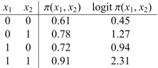
A similar situation occur in the following example, again with two binary covariates, but now with a binary outcome. The (true) model can be described by the following probabilities:
x1 x2 π(x1,x2) logitπ(x1,x2)
0 0 0.61 0.45
0 1 0.78 1.27
1 0 0.72 0.94
1 1 0.91 2.31
If we look at the probability values, we have exact additivity: π(1,0)= π(0,0)+0.11,π(0,1)=
π(0,0)+0.17, π(1,1) = π(0,0)+0.11+0.17. However, on the logit scale we have a distinct interaction, cf. Figure 18.13. Similar, in a Cox model we may have an interaction on the log hazard scale, which correspond to additivity on the hazard scale, or vice versa.
.6
.7
.8
.9
0 1
x2= 0
x2= 1
x1
π
(
x1
,
x2
)
.5
1
1
.5
2
2
.5
0 1
x2 =0
x2 =1
x1
lo
g
it
π
(
x1
,
x2
)
Figure 18.13: Illustrations of a simple model with additivity on the probability scale, but an interaction on the logit scale.
Hence in any interpretation of (quantitative) interactions or effect modification, one has to consider always the choice of the scale as one possible explanation. However, a change in the sign of the effect of a covariate, i.e. a qualitative interaction, is robust against monotone transformations of the scale, so here this explanation cannot be valid.
Remark:In the case of a continuous outcome, one may decide to transform the outcome variable if one feels that the standard scale is inadequate. However, here the same considerations as with transforming the outcome to obtain a better linear fit have to be applied (cf. Section 17.1).
18.8
Ceiling e
ff
ects and interactions
Many outcome variables cannot be decreased or increased to any degree. There may be biolog-ical bounds, e.g. a certain fat intake is necessary for human beings to survive. Many outcome variables are also bounded by the measurement instrument: For example if assessing the quality of life of a patient by scores computed from the marks on a questionnaire, a patient cannot score
18.9. HUNTING FOR INTERACTIONS 265
more than the maximal number of points. If there are now subjects in a study with values close to such a bound, they may be limited in showing a relation to covariates, as they cannot further improve or deteriorate. We then say that a regression analysis may suffer from ceiling (or floor)
effects.
Ceiling effects are often a source for interactions, as they may prevent one subgroups of
subjects to be sensitive to the covariate of interest. For example we may consider another study
in GPs looking at the effect of calling GPS to use more time on counseling in patients suffering
from depressions. In such an intervention study we may observe the following result with respect to rates of hospitalisation:
practice size
small large
control group 10.7% 33.4%
intervention group 10.1% 12.4%
OR 0.94 0.28
One may conclude that the intervention is working fine in GPs in large practices whereas in
small practices there is no effect. However, it is not allowed to interpret this in the way that
GPs in the small practices did not follow the suggestions of the intervention study or lacked compliance in another manner. As visible from the results in the control group GPs in small practice are already today good in handling patients with depressions and the intervention brings the GPs from large practices just up to the level of GPs from small practices. If we assume that 10% of all patients with depression are in general robust against treatment by GPs and can only be managed by hospitalisation, than the GPs in small practices had no chance to improve, and
hence no chance to show an effect of the intervention in contrast to the GPs from large practices.
So this interaction may be due to a floor effect of GPs in small practices.
So whenever one observes an interaction, one should take a closer look at the data and ask
oneself whether it may be due to a ceiling effect. If it can be explained this way, it does not
mean that the interaction is invalid or an artefact. It just means that one has to take the ceiling
effect into account in the subject matter interpretation of the interaction.
18.9
Hunting for interactions
From a general research methodological point of view it is highly desirable to detect existing interactions. If we use regression models to describe and understand the influence of several
covariates X1,X2, . . . ,Xp, interactions will make a major contribution to the understanding, as
the dependence of the effect of X1 on X2 may allow some insights into the mechanism how
X1influences the outcome. Qualitative interactions are of special importance, as they typically
challenge the traditional interpretation of covariates as universal risk factors in the particular setting. So this suggests to look systematically for interactions, whenever we fit a regression
Unfortunately an investigation of interactions or effect modification suffers usually from a poor power. Let us compare the situation of estimating the overall effectβ1of a covariateX1in a model without interactions with estimating the difference between the two subgroup specific effects βA1 and βB1, i.e. an interaction with a binary covariate X2. If 50% of our sample shows
X2 = 1 and the other halfX2 = 0, then each of the two estimates ˆβA1 and ˆβ B
1 are based on half of the data. This implies, that their standard errors are inflated by a factor of √2 in comparison to the standard error of ˆβ1. And taking the difference ˆβ1B−βˆA1 increases the standard error further by a factor of √2, such that the standard error of the difference ˆβ1B − βˆA1 is hence twice the standard error of ˆβ1. In the situation of a quantitative interaction, we may haveβ1A = 0.5β1and βA1 = 1.5β1, such thatβ1B−βA1 =β1, i.e. the parameter of interest is of the same magnitude in both situations. However, if our study has a power of 80% to reject the null hypothesisH0 :β1 = 0, it will have only a power of 29% to reject the null hypothesisH0 : βA1 = βB1 of no interaction due to the larger standard error of ˆβ1B−βˆA1. If we want to have a similar power for the detection of a difference in the sub group specific effects, we have to assume that the difference between βB1 andβ1A is twice asβ1, i.e. a rather extreme effect modification. And in most applications of regression models we are typically glad to have a sample size allowing to estimate the effect of the covariates with sufficient precision to prove that they have an effect, such that we cannot expect a large power to detect interactions.
The second problem with a systematic investigation of interactions is multiplicity. If we have 5 covariates, we have already 10 pairs of covariates, i.e. 10 interaction terms we can add (or even more, if some of the covariates are categorical). So if we just look at the resulting p-values, we cannot regard the significance of an interaction as a reliable indicator for its existence. One can find nevertheless sometimes the results of such a search in medical publications without any attempt to take the multiplicity problem into account, just reporting typically one significant interaction out of 10 or 20 tested. This is of no great value, and it is one example of the bad tradition of “hunting for p-values”.
So whenever one starts to think about investigating interactions systematically, one should be aware of that one tries something which has only a very limited chance to produce any reliable result. We have a rather low power to detect true interactions and simultaneously a high chance to produce false signals. To reduce the multiplicity problem the first step should be to define a (small) subset of all possible interactions or effect modifications, which are a priori of special interest or likely to indicate effect modifications of interest. There are three major sources to identify such interactions:
a) We may find hints on interactions in the literature. These may be due that authors have already investigated effect modification or that studies varying in important population characteristics vary with respect to their effect estimates of a covariate. Personal com-munications with experienced researchers in the field of interest may be a similar source, as they may have experienced that some traditional factors are of limited value in some subjects.
b) Certain effect modifications may be more plausible than others. Subject matter reasons may suggest that a factor has different meanings in different subgroups. For example in looking at the association between physical occupation and back pain as considered in
18.9. HUNTING FOR INTERACTIONS 267
Exercise 8.6, it will not be very surprising that the four categories of physical occupation may show a different effect in males and females due to differences in the physiology and biomechanics between women and men. In contrast, an interaction between social class and sex might be more difficult to explain.
c) If a study focus on a particular covariate, then interactions with this covariate are of higher interest than interactions among other covariates.
Once we have identified a very few of such interactions, we should include them as primary hypotheses in the study protocol, and if we succeed in confirming these hypothesis in the present study, we can include this as a result in our publication without being accused for extensive hunting for p-values. In addition, as a hypotheses generating part of the analysis, one may look systematically at all possible interactions.
In any case, any investigation of interactions should focus on the relevance of the implied effect modifications, not only just on the p-values of the interaction parameters. So a basis for the systematic investigation may be a table structured like that shown in Table 18.1.
effect effect of covariate
modifying age sex occupation ...
covariate βage βsex δˆblue vs. white δˆblue vs. others δˆwhite vs. others ...
effect at – ... ... ... ... ...
age of 30 [...,...] [...,...] [...,...] [...,...] ...
age effect at – ... ... ... ... ...
age of 70 [...,...] [...,...] [...,...] [...,...] ...
difference – ... ... ... ... ...
[...,...] [...,...] [...,...] [...,...] ...
effect ... – ... ... ... ...
in males [...,...] – [...,...] [...,...] [...,...] ...
sex effect ... – ... ... ... ...
in females [...,...] – [...,...] [...,...] [...,...] ...
difference ... – ... ... ... ...
[...,...] – [...,...] [...,...] [...,...] ...
effect for ... ... – – – ...
blue collar [...,...] [...,...] ...
effect for ... ... – – – ...
occupation white collar [...,...] [...,...] ...
effect for ... ... – – – ...
others [...,...] [...,...] ...
p-value ... ... – – – ...
... ... ... ... ... ... ... ...
Table 18.1: A proposal for a tabular presentation of relevant results for a systematic investiga-tion of interacinvestiga-tions.
18.10
How to analyse e
ff
ect modification and interactions with
Stata
We start with the example of Figure 18.1:
. clear
. use vitaminB . list
+---+ | dose sex weight | |---| 1. | 30 1 73 | 2. | 30 0 51 | 3. | 40 1 67 | 4. | 40 0 56 | 5. | 50 1 81 | |---| 6. | 50 0 53 | 7. | 70 1 93 | 8. | 70 0 58 | +---+
We define the two version of the covariatedose, one for the males and one for the females:
. gen dosemale=dose*(sex==1) . gen dosefemale=dose*(sex==0)
Now we can put this into a regression model:
. regress weight dosemale dosefemale sex
Source | SS df MS Number of obs = 8 ---+--- F( 3, 4) = 22.57 Model | 1472.97143 3 490.990476 Prob > F = 0.0057 Residual | 87.0285714 4 21.7571429 R-squared = 0.9442 ---+--- Adj R-squared = 0.9024 Total | 1560 7 222.857143 Root MSE = 4.6645
18.10. HOW TO ANALYSE EFFECT MODIFICATION AND INTERACTIONS WITH STATA269
---weight | Coef. Std. Err. t P>|t| [95% Conf. Interval] ---+---dosemale | .5885714 .1576874 3.73 0.020 .1507611 1.026382 dosefemale | .1428571 .1576874 0.91 0.416 -.2949532 .5806675 sex | 2.828571 11.09429 0.25 0.811 -27.97412 33.63126 _cons | 47.71429 7.844848 6.08 0.004 25.9335 69.49507
---We obtain directly the two sex specific effect estimates of the vitamin B intake. To assess the difference between the two effect estimates, we can use thelincomcommand.
. lincom dosemale-dosefemale ( 1) dosemale - dosefemale = 0
---weight | Coef. Std. Err. t P>|t| [95% Conf. Interval] ---+---(1) | .4457143 .2230036 2.00 0.116 -.173443 1.064872
---If we assume that we are also interested in showing that the vitamin B intake has any effect, we can perform the strategy discussed in Section 18.5 and look on the average dose effect:
. lincom 0.5*dosemale+0.5*dosefemale ( 1) .5*dosemale + .5*dosefemale = 0
---weight | Coef. Std. Err. t P>|t| [95% Conf. Interval] ---+---(1) | .3657143 .1115018 3.28 0.031 .0561356 .6752929
---So we have evidence for an effect of the dose. For illustrative purposes we also perform the alternative strategy to test the null hypothesis of no effect in both male and female mice:
. test dosemale dosefemale ( 1) dosemale = 0
F( 2, 4) = 7.38 Prob > F = 0.0455
Note that the p-value is bigger, reflecting the lower power of this approach.
If we want to follow the approach to add interaction terms, we can define the product of the
covariatesdoseandsexexplicitly
. gen dosesex=dose*sex
and add it to the regression model:
. regress weight dose sex dosesex
Source | SS df MS Number of obs = 8 ---+--- F( 3, 4) = 22.57 Model | 1472.97143 3 490.990476 Prob > F = 0.0057 Residual | 87.0285714 4 21.7571429 R-squared = 0.9442 ---+--- Adj R-squared = 0.9024 Total | 1560 7 222.857143 Root MSE = 4.6645 ---weight | Coef. Std. Err. t P>|t| [95% Conf. Interval] ---+---dose | .1428571 .1576874 0.91 0.416 -.2949532 .5806675 sex | 2.828571 11.09429 0.25 0.811 -27.97412 33.63126 dosesex | .4457143 .2230036 2.00 0.116 -.173443 1.064872 _cons | 47.71429 7.844848 6.08 0.004 25.9335 69.49507
---Note that the results fordosesexagree with those of the firstlincomcommand above.
To obtain the slope estimates within the two sex groups we have just to realize that within the females (sex==0) our model reads
µ(x1,0)=β˜0+β˜1x1
such that the effect of the vitamin B intake in females is equal to the effect ofdosein the output
above. Within males (sex==1) the model reads
µ(x1,1) = β˜0+β˜1x1+β˜2+β˜12x1 (18.1)
18.10. HOW TO ANALYSE EFFECT MODIFICATION AND INTERACTIONS WITH STATA271
such that the slope estimate for the males (sex==1) can be computed as
. lincom dose+dosesex ( 1) dose + dosesex = 0
---weight | Coef. Std. Err. t P>|t| [95% Conf. Interval] ---+---(1) | .5885714 .1576874 3.73 0.020 .1507611 1.026382
---The tests about any effect of the vitamin B intake can be performed by
. lincom 0.5*dose + 0.5*(dose+dosesex) ( 1) dose + .5*dosesex = 0
---weight | Coef. Std. Err. t P>|t| [95% Conf. Interval] ---+---(1) | .3657143 .1115018 3.28 0.031 .0561356 .6752929
---and by
. test dose dosesex ( 1) dose = 0 ( 2) dosesex = 0
F( 2, 4) = 7.38 Prob > F = 0.0455
One can also use Stata’s xi: construct to add the product of the covariates to the regression model:
. xi: regress weight i.sex*dose
i.sex _Isex_0-1 (naturally coded; _Isex_0 omitted) i.sex*dose _IsexXdose_# (coded as above)
---+--- F( 3, 4) = 22.57 Model | 1472.97143 3 490.990476 Prob > F = 0.0057 Residual | 87.0285714 4 21.7571429 R-squared = 0.9442 ---+--- Adj R-squared = 0.9024 Total | 1560 7 222.857143 Root MSE = 4.6645 ---weight | Coef. Std. Err. t P>|t| [95% Conf. Interval] ---+---_Isex_1 | 2.828571 11.09429 0.25 0.811 -27.97412 33.63126 dose | .1428571 .1576874 0.91 0.416 -.2949532 .5806675 _IsexXdose_1 | .4457143 .2230036 2.00 0.116 -.173443 1.064872 _cons | 47.71429 7.844848 6.08 0.004 25.9335 69.49507
---Note however that this does not work if both covariates are continuous.
We now consider the example of Figure 18.4.
. use hyper . list in 1/10
+---+ | id age smoking hyper | |---|
1. | 1 47 0 0 |
2. | 2 53 1 1 |
3. | 3 50 1 1 |
4. | 4 40 1 1 |
5. | 5 33 1 0 |
|---|
6. | 6 47 0 0 |
7. | 7 54 1 1 |
8. | 8 38 0 0 |
9. | 9 59 0 1 |
10. | 10 67 0 1 | +---+
and would like to investigate the effect ofsmokingas a function ofage. Sinceageis a continu-ous covariate, we have to follow the interaction approach:
18.10. HOW TO ANALYSE EFFECT MODIFICATION AND INTERACTIONS WITH STATA273
. gen agesmoking=age*smoking
. logit hyper age smoking agesmoking
Iteration 0: log likelihood = -877.28077 Iteration 1: log likelihood = -795.08929 Iteration 2: log likelihood = -793.22769 Iteration 3: log likelihood = -793.22413 Iteration 4: log likelihood = -793.22413
Logistic regression Number of obs = 1332 LR chi2(3) = 168.11 Prob > chi2 = 0.0000 Log likelihood = -793.22413 Pseudo R2 = 0.0958 ---hyper | Coef. Std. Err. z P>|z| [95% Conf. Interval] ---+---age | .0512461 .0064305 7.97 0.000 .0386426 .0638497 smoking | 2.955036 .5061917 5.84 0.000 1.962918 3.947153 agesmoking | -.0326584 .0087536 -3.73 0.000 -.0498152 -.0155016 _cons | -3.905869 .3847093 -10.15 0.000 -4.659885 -3.151852
---Now we can assess the change of the effect of smoking over 10 years
. lincom agesmoking*10
( 1) 10*[hyper]agesmoking = 0
---hyper | Coef. Std. Err. z P>|z| [95% Conf. Interval] ---+---(1) | -.3265839 .0875364 -3.73 0.000 -.4981521 -.1550156
---and we can use lincom’s or option to obtain the result as the factor corresponding to the increase of the odds ratio:
. lincom agesmoking*10, or ( 1) 10*[hyper]agesmoking = 0
---hyper | Odds Ratio Std. Err. z P>|z| [95% Conf. Interval] ---+---(1) | .7213839 .0631474 -3.73 0.000 .6076525 .8564018
---Now we look at the effect of smoking at age 35 and age 75:
. lincom _b[smoking] + 75 * _b[agesmoking]
( 1) [hyper]smoking + 75*[hyper]agesmoking = 0
---hyper | Coef. Std. Err. z P>|z| [95% Conf. Interval] ---+---(1) | .5056565 .2059231 2.46 0.014 .1020546 .9092584 ---. lincom _b[smoking] + 35 * _b[agesmoking]
( 1) [hyper]smoking + 35*[hyper]agesmoking = 0
---hyper | Coef. Std. Err. z P>|z| [95% Conf. Interval] ---+---(1) | 1.811992 .2217385 8.17 0.000 1.377393 2.246591
---Finally, we take a look at how to perform likelihood ratio tests. (Which are again slightly more powerful.) First we test the null hypothesis of no interaction by comparing the model above with a model without an interaction:
. estimates store A
. logit hyper age smoking
Iteration 0: log likelihood = -877.28077 Iteration 1: log likelihood = -801.10435 Iteration 2: log likelihood = -800.2788 Iteration 3: log likelihood = -800.27872
Logistic regression Number of obs = 1332 LR chi2(2) = 154.00 Prob > chi2 = 0.0000
18.10. HOW TO ANALYSE EFFECT MODIFICATION AND INTERACTIONS WITH STATA275
Log likelihood = -800.27872 Pseudo R2 = 0.0878 ---hyper | Coef. Std. Err. z P>|z| [95% Conf. Interval] ---+---age | .0344195 .0043207 7.97 0.000 .0259511 .0428878 smoking | 1.139242 .1214511 9.38 0.000 .901202 1.377281 _cons | -2.936872 .2597851 -11.31 0.000 -3.446042 -2.427703 ---. lrtest A
Likelihood-ratio test LR chi2(1) = 14.11 (Assumption: . nested in A) Prob > chi2 = 0.0002
Next we test the null hypothesis of “no effect of smoking at all” by comparing the full model with the model in which all terms involvingsmokingare omitted:
. logit hyper age
Iteration 0: log likelihood = -877.28077 Iteration 1: log likelihood = -846.18595 Iteration 2: log likelihood = -846.07003 Iteration 3: log likelihood = -846.07002
Logistic regression Number of obs = 1332 LR chi2(1) = 62.42 Prob > chi2 = 0.0000 Log likelihood = -846.07002 Pseudo R2 = 0.0356 ---hyper | Coef. Std. Err. z P>|z| [95% Conf. Interval] ---+---age | .0320192 .0041419 7.73 0.000 .0239012 .0401373 _cons | -2.278813 .2361742 -9.65 0.000 -2.741706 -1.81592 ---. lrtest A
Likelihood-ratio test LR chi2(2) = 105.69 (Assumption: . nested in A) Prob > chi2 = 0.0000
18.11
Exercise
Treatment interactions in a randomised clinical
trial for the treatment of malignant glioma
The datasetgliomincludes data from a randomised clinical trial comparing a mono chemother-apy (BCNU) with a combination therchemother-apy (BCNU + VW 26) for the treatment of malignant glioma in adult patients. The variabletimeincludes the survival time (in days) after chemother-apy (ifdied==1), or the time until the last contact with the patient (ifdied==0).
a) It has been claimed that the benefit from the combination therapy depends on the per-formance status of the patient. The variablepsdivides the subjects into those with poor performance status (ps==0) and those with good performance status (ps==1). Try to clar-ify the claim based on the available data. Try to support the results of your analysis by appropriate Kaplan Meier curves.
b) Some people have even raised doubt about that the combination therapy is of any benefit for the patients. Try to clarify this question based on the available data.
c) It has been claimed that the benefit from the combination therapy depends on the age of the patient. Try to clarify this claim based on the available data. Try to support the results of your analysis by appropriate Kaplan Meier curves.
d) The dataset includes besides the variable psalso a variable karnindex, which divides the subjects into three groups according to their Karnofsky index, a more detailed mea-surement of the performance status. Try to reanalyse a) again using this variable. Try to support the results of your analysis by appropriate Kaplan Meier curves.