By SUSANTOBASU, JOHN G. FERNALD, ANDMILES S. KIMBALL*
Yes. We construct a measure of aggregate technology change, controlling for aggregation effects, varying utilization of capital and labor, nonconstant returns, and imperfect competition. On impact, when technology improves, input use and nonresidential investment fall sharply. Output changes little. With a lag of several years, inputs and investment return to normal and output rises strongly. The standard one-sector real-business-cycle model is not consistent with this evidence. The evidence is consistent, however, with simple sticky-price models, which predict the results we find: when technology improves, inputs and investment generally fall in the short run, and output itself may also fall.(JELE22, E32, O33)
When technology improves, does employ-ment of capital and labor rise in the short run? Although standard frictionless real-business-cycle (RBC) models generally predict that they do, other macroeconomic models predict the opposite. For example, sticky-price and imper-fect-information models often predict that tech-nology improvements cause employment to fall in the short run, when prices are fixed, but rise
in the long run, when prices change. These models also imply that technology improve-ments could, by reducing short-run investment demand, cause a short-run decline in output as well as inputs. Hence, correlations among tech-nology, inputs, investment, and output shed light on the merits of different business-cycle models.
Measuring these correlations requires an ap-propriate measure of aggregate technology. We construct such a series by controlling for non-technological effects in aggregate total factor productivity (TFP): varying utilization of capi-tal and labor, nonconstant returns and imperfect competition, and aggregation effects.1 “Puri-fied” technology varies about half as much as TFP. Technology shocks appear permanent and do not appear serially correlated.
We find that technology improvements re-duce total hours worked within the year, but increase hours with a lag of up to two years. Output changes little on impact, but increases strongly thereafter. Nonresidential investment falls sharply on impact before rising above its steady-state level. Household spending (espe-* Basu: Department of Economics, Boston College, 140
Commonwealth Avenue, Chestnut Hill, MA 02467-3806, and National Bureau of Economic Research (e-mail: [email protected]); Fernald: Economic Research MS 1130, Federal Reserve Bank of San Francisco, 101 Market Street, San Francisco, CA 94105 (e-mail: [email protected]); Kimball: Department of Economics, University of Michi-gan, 611 Tappan Street, Ann Arbor, MI 41809-1220, and NBER (e-mail: [email protected]). For comments and advice, we thank Robert Barsky, Jeffrey Campbell, Menzie Chinn, Russell Cooper, Martin Eichenbaum, Charles Evans, Jonas Fisher, Barbara Fraumeni, Christopher Foote, Jordi Galı´, Zvi Griliches, Robert Hall, Dale Henderson, Dale Jorgenson, Michael Kiley, Lutz Kilian, Robert King, Serena Ng, Jonathan Parker, Shinichi Sakata, Matthew Shapiro, Robert Solow, Jeffrey Wooldridge, Jonathan Wright, and seminar participants at a number of institutions and confer-ences. We also thank several anonymous referees. This is a very substantially revised version of papers previously cir-culated as Federal Reserve International Finance Discussion Paper No. 625 and Harvard Institute of Economic Research Discussion Paper No. 1986. Basu and Kimball gratefully acknowledge support from a National Science Foundation grant to the NBER. Basu also thanks the Alfred P. Sloan Foundation for financial support. We particularly thank Shanthi Ramnath, as well as Chin Te Liu, Andrew McCal-lum, David Thipphavong and Stephanie Wang, for superb research assistance. This paper represents the views of the authors and does not necessarily reflect the views of anyone else associated with the Federal Reserve System.
1Unless we specifically state otherwise, we use
“tech-nology” and “TFP” to refer to growth in these variables. We define TFP to be the standard Solow residual: output growth minus revenue-share-weighted input growth, which need not measure technology. We note that Robert M. Solow’s (1957) original article suggests modifications and exten-sions (for example, for factor utilization and monopoly power) necessary for his residual to properly measure tech-nology at business cycle frequencies; he also notes the issue of aggregation. Basu and Fernald (2001) discuss additional references on technology and TFP.
cially durable consumption and residential in-vestment) rises on impact and rises further with a lag. Thus, after a year or two, the response to our estimated technology series more or less matches the predictions of the standard, fric-tionless RBC model. But the short-run effects do not.
Correcting for unobserved input utilization (labor effort and capital’s workweek) is central to understanding the relationship between pro-cyclical TFP and counterpro-cyclical purified tech-nology. Utilization is a form of primary input. Our estimates imply that when technology im-proves, unobserved utilization, as well as ob-served inputs, fall sharply on impact. Both then recover with a lag. In other words, when tech-nology improves, utilization falls—so TFP ini-tially rises less than technology does.
Of course, if technology shocks were the only impulse—and if, as we estimate, these shocks were negatively correlated with the cycle—then even before controlling for utilization, we would still be likely to observe a negative cor-relation between uncorrected TFP and the busi-ness cycle. Demand shocks can explain why, instead, uncorrected TFP is procyclical. When demand increases, output and inputs—including unobserved utilization—increase as well. We find that nontechnology shocks are important enough at cyclical frequencies for changes in utilization to make uncorrected TFP procyclical.
To identify technology, we use tools from Basu and Fernald (1997) and Basu and Kimball (1997), who in turn build on Solow (1957) and Robert E. Hall (1990). Basu and Fernald stress the role of sectoral heterogeneity and aggrega-tion. They argue that for economically plausible reasons—for example, differences across indus-tries in the degrees of market power—the mar-ginal product of an input may differ across uses. The aggregate Solow residual (growth in aggre-gate TFP) then depends on which sectors change input use the most over the business cycle. Basu and Kimball stress the role of vari-able capital and labor utilization. Their basic insight is that a cost-minimizing firm operates on all margins simultaneously, both observed and unobserved. Hence, changes in observed inputs can proxy for unobserved utilization changes. For example, if labor is particularly valuable, firms will tend to work existing em-ployees both longer (observed hours per worker rise) and harder (unobserved effort rises).
Together, these two papers imply that one can construct an index of aggregate technology change by “purifying” sectoral Solow residuals and then aggregating across sectors. Thus, our fundamental identification comes from estimat-ing sectoral production functions.
Jordi Galı´ (1999a) independently proposes a quite different method to investigate similar issues. Following Olivier J. Blanchard and Danny Quah (1989) and Matthew D. Shapiro and Mark W. Watson (1988), Galı´ identifies technology shocks using long-run restrictions in a structural vector autoregression (SVAR). Galı´ assumes that only technology shocks af-fect labor productivity in the long run. He examines aggregate data on output and hours worked for a number of countries and, like us, finds that technology shocks reduce input use on impact.
A growing literature questions or defends Galı´’s (1999a) specification.2 Neville Francis
and Valerie A. Ramey (2005) extend Galı´’s identification scheme and subject it to a range of economic and statistical tests; they conclude that “the original technology-driven real busi-ness cycle hypothesis does appear to be dead.” Lawrence J. Christiano et al. (2003), however, argue for using per capita hours in log-levels rather than in growth rates. With this subtle change in specification, they conclude that tech-nology improvements raise hours worked on impact.3 Thus, although the SVAR evidence mostly suggests that technology improvements reduce hours, the evidence from this approach is not yet conclusive.
Our alternative augmented-growth-account-ing approach relies on completely different as-sumptions for identification, with at least four advantages relative to the SVAR literature. First, our results do not depend on a theoret-ically derived long-run identifying restriction that might not hold. For example, increasing returns, permanent sectoral shifts, capital
2See Galı´ and Pau Rabanal (2005) for a recent summary. 3Fernald (2005) argues that the specification of
Chris-tiano et al. (2004) also implies that technology improve-ments reduce hours worked, once one controls for the early 1970s productivity slowdown and mid-1990s acceleration in productivity. (Christiano et al., 2005, and related work by David Altig et al., 2005, make several important method-ological contributions to the literature that we view as more substantive than their specific empirical results.) We discuss several related points in Section IV.
taxes, and some models of endogenous growth would all imply that nontechnology shocks can change long-run labor productiv-ity, thus invalidating the identifying assump-tion.4 Our production-function approach
allows these deviations. Second, we can iden-tify transitory as well as permanent technol-ogy shocks; the SVAR approach, in contrast, at best identifies only permanent, unit-root technology shocks. Third, even if the long-run restriction holds, it produces well-identi-fied shocks and reliable inferences only with potentially restrictive, atheoretical auxiliary assumptions (see, for example, Jon Faust and Eric M. Leeper, 1997).5Our
production-func-tion approach, by contrast, does not rely on these same identification conditions. Fourth, we can easily look at the effect of technology shocks on a large number of variables; results from an identified VAR might look very dif-ferent as more variables are added. Never-theless, we view the identified VAR and augmented-growth-accounting approaches as complements, with distinct identification schemes and strengths.
Two additional approaches also suggest that technology improvements reduce input use. First, estimated structural dynamic general equilibrium (DGE) models (for example, Frank Smets and Raf Wouters, 2003, for the euro area and Andrew Levin et al., 2006, for the United States) often find that technology improvements reduce input use on impact. Second, John Shea (1999) measures tech-nology as innovations to R&D spending and patent activity and finds that with a lag of several years process innovations increase TFP and si-multaneously lower labor input.6
Despite differing data, countries, and meth-ods, the bottom line is that the state-of-the-art
versions of four very different approaches yield similar results. We thus view the contractionary effect of technology improvements as a robust stylized fact that models need to explain.
What do these results imply for modeling business cycles? They are clearly inconsistent with standard parameterizations of frictionless RBC models, including Robert G. King and Sergio T. Rebelo’s (1999) attempt to “resusci-tate” these models. The negative effect of a technology improvement on nonresidential in-vestment is particularly hard to reconcile with flexible-price RBC models (including the mod-els suggested by Francis and Ramey, 2003), given our finding that technology appears to be a random walk. Our findings are consistent, however, with the predictions of DGE models with sticky prices. Consider the quantity-theory case where output is proportional to real bal-ances. In the short run, if the supply of money is fixed and prices cannot adjust, then real bal-ances and hence output are also fixed. Now suppose technology improves. Firms now need fewer inputs to produce this unchanged output, so they lay off workers and desire less capital, which could reduce investment.7 Over time, however, prices adjust, the underlying RBC dy-namics take over, and output rises. Relaxing the quantity-theory assumption allows for richer dynamics for output (which could even decline) and its components, but doesn’t change the ba-sic message. Models where price rigidity arises endogenously from imperfect common knowl-edge, as in Michael Woodford (2003a), make similar predictions (see Takuji Kawamoto, 2004).
Of course, in a sticky-price model, technol-ogy improvements will be contractionary only if the monetary authority does not offset their short-run effects through expansionary mone-tary policy. After all, standard sticky-price mod-els predict that a technology improvement that increases full-employment output creates a short-run disinflation, which gives the monetary authority room to lower interest rates. In Sec-tion V, we argue that technology improvements are still likely to be contractionary, reflecting
4Gadi Barlevy (2004) models cyclical fluctuations as
having a substantial effect on long-run growth. In the SVAR context, Harald Uhlig (2004) discusses capital taxes and time-varying attitudes toward workplace leisure; Pierre-Daniel Sarte (1997) suggests that hysteresis in labor quality might lead demand shocks to have permanent productivity effects.
5Thomas F. Cooley and Mark Dwyer (1998) and
Chris-topher J. Erceg et al. (2005) estimate SVARs on data from calibrated DGE models and suggest that these concerns could, in some cases, be important. Erceg et al. do conclude that SVAR results can be informative.
6Galı´ (1999b) draws out and discusses this implication
of Shea’s findings.
7James Tobin (1955) makes this point in a model with
the fact that central banks observe technology shocks only with a long lag.8
Clearly, our results are not a “test” of sticky-price or sticky-information models of business cycles, even though the results are consistent with that interpretation. We favor this interpre-tation in part because one wants a model that appropriately captures the economy’s response to both monetary and real shocks, and models with endogenous or exogenous price rigidity can generate large monetary nonneutralities. Other possible explanations include a flexible-price world with autocorrelated technology shocks, low capital-labor substitutability, or substantial real frictions such as habit persis-tence in consumption and investment adjust-ment costs; sectoral shifts, if reallocations are correlated with technology growth; the need to learn about new technologies; and “cleansing effects” of recessions, in which recessions lead firms to reorganize or, within an industry, elim-inate low-productivity firms. We discuss a range of alternative explanations in Section V. The paper has the following structure. Sec-tion I reviews our method for identifying sec-toral and aggregate technology change. Section II discusses data and econometric method. tion III presents our main empirical results. Sec-tion IV discusses robustness. SecSec-tion V presents alternative interpretations of our results, includ-ing our preferred sticky-price interpretation. Section VI concludes.
I. Estimating Aggregate Technology, Controlling for Utilization
We identify aggregate technology by estimat-ing (instrumented) a Hall-style regression equa-tion with a proxy for utilizaequa-tion in each disaggregated industry. We then define aggre-gate technology change as an appropriately weighted sum of the resulting residuals. Section IA discusses our augmented Solow-Hall ap-proach and aggregation; Section IB discusses how we control for utilization.
A. Industry and Aggregate Technology We assume each industry has a production function for gross output:
(1) Yi⫽F i共
AiKi,EiHiNi,Mi,Zi兲.
The industry produces gross output, Yi, using
the capital stock Ki, employees Ni, and
inter-mediate inputs of energy and materialsMi. We
assume that the capital stock and number of employees are quasi-fixed, so their levels can-not be changed costlessly. But industries may vary the intensity with which they use these quasi-fixed inputs:Hiis hours worked per
em-ployee;Eiis the effort of each worker; andAiis
the capital utilization rate (that is, capital’s workweek). Total labor input,Li, is the product
EiHiNi. The production functionFi is (locally)
homogeneous of arbitrary degree ␥i in total inputs;␥iexceeding one implies increasing returns to scale, reflecting overhead costs, decreasing marginal cost, or both;Ziindexes technology.
Following Hall (1990), we assume cost min-imization and relate output growth to the growth rate of inputs. The standard first-order condi-tions give us the necessary output elasticities, i.e., the weights on growth of each input.9Let dxi be observed input growth, and dui be
unobserved growth in utilization. (For any vari-able J, we define dj as its logarithmic growth rate ln(Jt/Jt⫺1).) This yields:
(2) dyi⫽␥i共dxi⫹dui兲⫹dzi,
where
(3) dxi⫽sKidki⫹sLi共dni⫹dhi兲⫹sMidmi,
dui⫽sKidai⫹sLidei,
andsJiis the ratio of payments to inputJin total
cost. Section IB explores ways to measuredui.
With constant returns, perfect competition, and no utilization changes, technology change dzi
equals the standard Solow residual (TFP):dzi⫽
d yi⫺ dxi.
8This assumption is quite natural in sticky-information
models, where it amounts to assuming that the central bank and the public have the same information set. See Kawamoto (2004).
9Basu and Fernald (2001) provide detailed derivations
and discussion of the equations that follow. Note that with increasing returns, firms must charge a markup of price over marginal cost to cover their total costs. Hence, the resulting estimating equation controls for imperfect competition as well as increasing returns.
We define “purified” technology change as a weighted sum of industry technology change:
(4) dz⫽
冘
i
冉
wi
1⫺sMi
冊
dzi,
where wi equals (PiYi ⫺ PMiMi)/¥i (PiYi ⫺
PMiMi) ⬅ Pi V
Vi/P V
V, the industry’s share of aggregate nominal value added. Conceptually, dividing through by 1 ⫺ sM converts
gross-output technology shocks to a value-added basis (desirable because of the national accounts identity that aggregate final expenditure equals aggregate value added). These shocks are then weighted by the industry’s share of aggregate value added.10
We define changes in aggregate utilization as the contribution to final output of changes in in-dustry-level utilization. This, in turn, is a weighted average of industry-level utilization changes:
(5) du⫽
冘
i
冉
wi
1⫺sMi
冊
␥ idui.From equation (2), ␥idui enters in a manner
parallel todzi, so that (5) parallels (4).
Implementing this approach requires disag-gregated estimates of returns to scale and of variations in utilization. We observe all other variables necessary to calculate aggregate tech-nology and utilization.
B. Measuring Industry-Level Capital and Labor Utilization
Utilization growth,dui, is a weighted sum of
growth in capital utilization, Ai, and labor
ef-fort,Ei. Since cost-minimizing firms operate on
all margins simultaneously, changes in ob-served inputs can potentially proxy for unob-served utilization changes. We derive such a relationship from the cost-minimization condi-tions of the representative firm within each
in-dustry, following Basu and Kimball (1997). The model below provides microfoundations for a simple proxy: changes in hours-per-worker are proportional to unobserved changes in both la-bor effort and capital utilization. We assume only that firms minimize cost and are price-takers in factor markets; we do not require any assumptions about firms’ pricing and output behavior in the goods market. In addition, we do not assume that we observe the firm’s internal shadow prices of capital, labor, and output at high frequencies.
We model firms as facing adjustment costs to investment and hiring, so that capital (number of machines and buildings),K, and employment (number of workers), N, are both quasi-fixed. One needs quasi-fixity for a meaningful model of variable factor utilization. Higher utilization must raise firms’ costs, or they would always utilize factors fully. Given these costs, if firms could costlessly change the rate of investment or hiring, they would always keep utilization at its long-run cost-minimizing level and vary in-puts by hiring/firing workers and capital. Thus, only if it is costly to adjust capital and labor is it sensible to pay the costs of varying utilization.11
We assume that firms can freely vary A,E, andHwithout adjustment cost. We assume the major cost of increasing capital utilization,A, is that firms pay a shift premium (a higher wage) to compensate employees for working at night or other undesirable times. We take A to be a continuous variable for simplicity, although dis-crete variations in capital’s workday (the num-ber of shifts) are an important mechanism for varying utilization.12When firms increase labor utilization, E, they must compensate workers for the increased disutility of effort with a higher wage. High-frequency fluctuations in this wage might be unobserved if an implicit contract gov-erns wage payments in a long-term relationship.
10This weighting scheme follows Evsey Domar (1961).
In previous work, we defined aggregate technology with (1⫺␥isMi) in the denominator. This definition is convex in␥i. Indeed, as ␥sM 3 1, [1/(1⫺ ␥sM)] 3⬁. This means that positive and negative estimation error does not cancel out. Domar-weighted residuals are thus more robust to mismeasurement.
11As Trygve Haavelmo (1960) observes, one-sector
models can treat variable utilization withoutinternal adjust-ment costs, since the representative firm’s input demand affects the economy-wide real wage and interest rate. But internal adjustment costs are required to model why indus-tries vary utilization in response to idiosyncratic changes in technology or demand.
12J. Joseph Beaulieu and Joseph Mattey (1998) and
Shapiro (1996), for example, apply the variable-shifts model to manufacturing.
An industry’s representative firm minimizes the present value of expected costs:
(6) min
A,E,H,M,I,D
Et
冘
⫽t⬁
冋
j写
⫽t⫺1
(1⫹rj)⫺1
册
⫻关WG共H,E兲V共A兲N⫹PM,M⫹WN⌿共D/N兲⫹PI,KJ共I/K兲兴
subject to
(7) Y⫽F共AK,EHN,M,Z兲; (8) K⫹1⫽I⫹共1⫺␦兲K;
(9) N⫹1⫽N⫹D.
In (6), we use the convention that the product of discount factors is equal to 1 when⫽t. In each period, the firm’s costs in (6) are total payments for labor and material, and the costs associated with undertaking gross investment I and hiring (net of separations) D. WG(H, E)V(A) is total compensation owed per worker (which, if it takes the form of an implicit contract, may not be ob-served period by period).Wis the base wage; the functionGspecifies how the hourly wage depends on effort,E, and the length of the workday,H; and V(A) is the shift premium. PM is the price of
materials.WN⌿(D/N) is the total cost of changing the number of employees;PIKJ(I/K) is the total
cost of investment; and␦is the rate of deprecia-tion. We assume that⌿andJare convex.13We omit time and industry subscripts except where needed for clarity.
There are six intra-temporal first-order con-ditions and Euler equations for each of the two state variablesKandN. The multiplier on con-straint (7),, represents marginal cost.Fj,j⫽1,
2, 3 denotes derivatives of F with respect to
argumentj, and literal subscripts denote deriv-atives of the labor cost functionG. To conserve space, we analyze only the optimization condi-tions that affect our derivacondi-tions, which are those for A,H, andE:
(10) A: F1K⫽WNG共H,E兲V⬘共A兲;
(11) H: F2EN⫽WNGH共H,E兲V共A兲;
(12) E: F2HN⫽WNGE共H,E兲V共A兲.
Note that uncertainty does not affect our derivations, which rely only on intra- tempo-ral optimization equations. Uncertainty af-fects the evolution of the state variables (as the Euler equations would show) but not the minimization of variable cost at a point in time, conditional on the levels of the state variables.
Equations (11) and (12) can be combined into an equation implicitly relatingEandH: (13) HGH共H,E兲
G共H,E兲 ⫽
EGE共H,E兲
G共H,E兲 .
The elasticities of labor costs with respect to H and E must be equal because, in terms of benefits, elasticities of effective labor input with respect to H andE are equal. Given the assumptions on G, (13) implies a unique, upward-sloping E-H expansion path: E ⫽ E(H), E⬘(H) ⬎ 0. That is, we can express unobserved intensity of labor utilization E as a function of observed hours per worker H. We define ⬅ H*E⬘(H*)/E(H*) as the elasticity of effort with respect to hours, evaluated at the steady state. Log-linearizing, we find:
(14) de⫽dh.
To find a proxy for capital utilization, we combine (10) and (11). Rearranging, we find: (15) F1AK/F
F2EHN/F⫽
冋
G(H,E) HGH(H,E)
册冋
AV⬘(A) V(A)
册
. The left-hand side is a ratio of output elastici-ties. As in Hall (1990), cost minimization im-plies that they are proportional to factor cost shares, which we denote by ␣Kand␣L. Define13We make necessary technical assumptions onGin the
spirit of convexity and normality. The conditions onGare easiest to state in terms of the function⌽defined by lnG(H, E)⫽ ⌽(lnH, lnE). Convex⌽guarantees a global optimum; assuming⌽11⬎ ⌽12and⌽22⬎ ⌽12ensures that there is only
one possible optimal value ofEfor each value ofH. We make some normalizations relative to normal or “detrended steady state” levels. LetJ(␦)⫽␦,J⬘(␦)⫽1, and⌿(0)⫽0. We also assume that the marginal employment adjustment cost is zero at a constant level of employment:⌿⬘(0)⫽0.
g(H) as the elasticity of labor cost with respect to hours: g(H) ⫽ HGH(H, E(H))/G(H, E(H)).
Definev(A) as the elasticity of labor cost with respect to capital’s workweek (equally, the ratio of the marginal to the average shift premium):
v(A)⫽ AV⬘(A)/V(A). We can then write equa-tion (15) as:
(16) v共A兲⫽共␣K/␣L兲g共H兲.
The functiong(H) is positive and increasing by the assumptions we have made onG(H,E); let
denote the (steady-state) elasticity of gwith respect toH. The functionv(A) is positive if the shift premium is positive. We assume that the shift premium increases rapidly enough withA to make the elasticity increasing inA. Letbe this elasticity ofv. We also assume that␣K/␣Lis constant, which requires thatFbe a generalized Cobb-Douglas function inKandL.14 The
log-linearization of (16) is simply (17) da⫽共/兲dh.
Equations (17) and (14) say that the change in hours per worker proxies for changes in both unobservable labor effort and the unmeasured workweek of capital. Hours per worker proxies for capital utilization as well as labor effort because shift premia create a link between cap-ital hours and labor compensation. The shift premium is most worth paying when the mar-ginal hourly cost of labor is high relative to its average cost, which occurs when hours per worker are also high.
Putting everything together, we have a simple estimating equation that controls for variable utilization:
(18) dy⫽␥dx⫹␥
冉
sL⫹ sK
冊
dh⫹dz⫽␥dx⫹dh⫹dz.
We will not need to identify all of the parame-ters in the coefficient multiplying dh, so we denote that composite coefficient by . This specification controls forbothlabor and capital
utilization.15 We measure industry technology
change as the residualsdz.
After estimating equation (18) on disagggated data, which controls for nonconstant re-turns, imperfect competition, and utilization, we aggregate as in (4) to get a measure of “puri-fied” aggregate technology.
II. Data and Method
A. Data
We seek to measure true aggregate technology change, dz, by estimating disaggregated technol-ogy change and then aggregating up to the private nonfarm, nonmining U.S. economy. We use in-dustry data from Dale Jorgenson and collaborators from 1949 to 1996. The data comprise 29 indus-tries (including 21 manufacturing indusindus-tries at roughly the two-digit level) that cover the entire nonfarm, nonmining private economy. These sec-toral accounts include industry gross output and inputs of capital, labor, energy, and materials. The Appendix describes the data and our calculations in more detail.
Given the potential correlation between input growth and technology shocks in equation (18), we use instruments uncorrelated with technology change. We use updated versions of two of the Hall-Ramey instruments: oil prices and growth in real government defense spending. For oil, we use increases in the U.S. refiner acquisition price. Our third instrument updates Burnside’s (1996) quar-terly Federal Reserve “monetary shocks” from an identified VAR. For all three instruments, we use the sum of the yeart⫺1 quarterly shocks as the instrument for yeart.16
14Thus, we assumeY⫽Z⌫((AK)␣K(EHN)␣L,M), where
⌫is a monotonically increasing function.
15As in Basu and Kimball (1997), allowing capital
utiliza-tion to affect depreciautiliza-tion would add two more terms. We cannot reject that these terms are zero; in any case, including them has little effect on results reported below. An alternative approach assumes, more restrictively, fixed proportions between an observed and unobserved input. For example, Craig Burnside et al. (1995, 1996) follow Dale Jorgenson and Zvi Griliches (1967) and Alfred W. Flux (1913) and suggest that electricity use might proxy for true capital services. This might be reasonable for some manufacturing industries, but it ignores labor effort and is probably more appropriate for heavy equipment than structures.
16The qualitative features of the results in Section III
appear robust to different combinations and lags of the instru-ments. An on-line Appendix (available from theAERWeb site at http://www.e-aer.org/data/dec06/20040577_app.pdf) discusses several econometric issues, including the small-sample properties of instrumental variables.
B. Estimating Technology Change We estimate industry-level technology change from the 29 regression residuals from (18), esti-mated as a system of equations. To conserve pa-rameters, we restrict the utilization coefficient within three groups: durables manufacturing (11 industries, listed in Table 1); nondurables manu-facturing (10); and nonmanumanu-facturing (8). Wald and quasi-likelihood ratio tests do not reject these constraints. (Without the constraints, the variance of estimated technology rises but qualitative and, indeed, quantitative results change little.) Thus, for the industries within each group, we estimate (19) dyi⫽ci⫹␥idxi⫹dhi⫹dzi.
This parsimonious equation controls for both capital and labor utilization. Note that
hours-per-worker growth dh essentially enters twice, since it is also in observed input growthdx. We allow returns-to-scale ␥ito differ by industries within a group. (Hypothesis tests overwhelm-ingly reject constraints on the ␥i). Aggregate “purified” technology change is the weighted sum of the industry residuals plus constant terms. Given the mid-sample productivity slowdown, we used Donald Andrews’s (1993) approach to test for a break in the industry constants. We imposed the restriction that any break is common to all industries within each group. Only in non-manufacturing do we reject the null of no break; for TFP growth, the maximum F statistic for a break corresponds to 1973 (just exceeding the value for 1967). We imposed a 1973 break in what follows; our main results appear little af-fected by adding this break or by changing the break date.
TABLE1—PARAMETERESTIMATES
Durable manufacturing Nondurable manufacturing Nonmanufacturing A. Returns-to-scale(␥i)estimates
Lumber (24) 0.51 Food (20) 0.84 Construction (15–17) 1.00
(0.08) (0.20) (0.07)
Furniture (25) 0.92 Tobacco (21) 0.90 Transportation (40–47) 1.19
(0.05) (0.27) (0.10)
Stone, clay, & glass (32) 1.08 Textiles (22) 0.64 Communication (48) 1.32
(0.04) (0.11) (0.21)
Primary metal (33) 0.96 Apparel (23) 0.70 Electric utilities (491) 1.82
(0.05) (0.08) (0.21)
Fabricated metal (34) 1.16 Paper (26) 1.02 Gas utilities (492) 0.94
(0.06) (0.10) (0.06)
Nonelectrical machinery (35) 1.16 Printing & publishing (27) 0.87 Trade (50–59) 1.01
(0.09) (0.19) (0.21)
Electrical machinery (36) 1.11 Chemicals (28) 1.83 FIRE (60–66) 0.65
(0.09) (0.16) (0.22)
Motor vehicles (371) 1.07 Petroleum products (29) 0.91 Services (70–89) 1.32
(0.05) (0.19) (0.25)
Other transport (372–79) 1.01 Rubber & plastics (30) 0.91
(0.03) (0.09)
Instruments (38) 0.95 Leather (31) 0.11
(0.11) (0.19)
Miscellaneous manufacturing (39) 1.17 (0.17)
Column average 1.01 0.87 1.16
Median 1.07 0.89 1.10
B. Coefficient on hours per worker
Durables 1.34 Nondurables 2.13 Nonmanufacturing 0.64
Manufacturing (0.22) Manufacturing (0.38) (0.34)
Notes:Heteroskedasticity- and autocorrelation-robust standard errors in parentheses. Coefficients from regression of output growth on input growth and hours-per-worker growth. (Constant terms and, for nonmanufacturing, post-1972 dummy, not shown.) Hours-per-worker coefficient is constrained to be equal within groups (durables, nondurables, and nonmanufactur-ing). Instruments are oil price increases; growth in real defense spending; and VAR monetary innovations. FIRE is finance, insurance, and real estate.
In addition, results are robust to using (uncon-strained) industry-by-industry estimation, either by 2SLS or LIML. Parameter estimates are less precise and more variable with individual than group estimation, but median estimates are similar to the median GMM estimates. Estimating indi-vidual equations raises the variance of estimated aggregate technology but does not change our main conclusions.
III. Results
A. Estimates and Summary Statistics Our main focus is the aggregate effects of tech-nology shocks, estimated as an appropriately weighted average of industry regression residuals. Table 1 summarizes the underlying industry pa-rameter estimates from equation (19). For durable manufacturing, the median returns-to-scale esti-mate is 1.07; for nondurable manufacturing, 0.89; for nonmanufacturing, 1.10. For all 29 industries shown, the median estimate is 1.00. (Omitting hours-per-worker growth raises the overall me-dian estimate of returns to scale to 1.12). After correcting for variable utilization, there is thus little overall evidence of increasing returns, al-though there is wide variation across industries.17
Throwing out “outlier” industries (lumber, tex-tiles, chemicals, leather, electric utilities, FIRE, and services) has little effect on results below.
The coefficient on hours-per-worker, in the bottom panel, is strongly statistically significant in durables and nondurables manufacturing.
The coefficient is significant at the 10-percent level in nonmanufacturing.
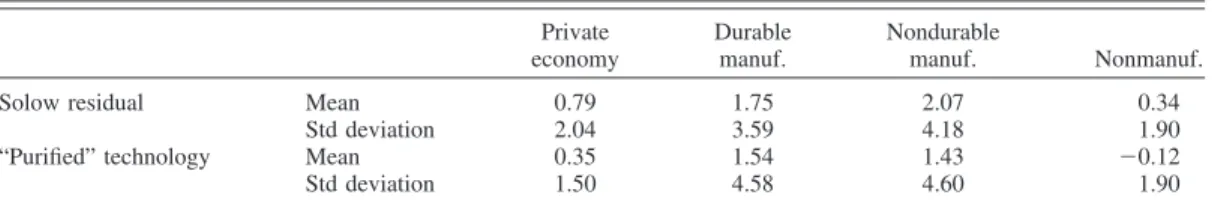
Table 2 summarizes means and standard de-viations for TFP (the Solow residual) and “pu-rified” technology. TFP does not adjust for utilization or nonconstant returns. Purified tech-nology controls for utilization and nonconstant returns, aggregated as in equation (5).
For the entire private nonmining economy, the standard deviation of technology, 1.5 percent per year, compares with the 2.0-percent standard de-viation of TFP; indeed, the variance is only 55 percent as high. For both durable and nondurable manufacturing, the standard deviation of purified technology is, perhaps surprisingly, higher than for TFP. The reduction in variance in column 1 comes primarily from reducing the (substantial) positive covariance across industries, consistent with the notion that business cycle factors— com-mon demand shocks—lead to positively corre-lated changes in utilization and TFP across industries.
Some simple plots summarize the comove-ment in our data. Figure 1 plots business-cycle data for the private economy: growth in TFP, output (aggregate value added), and hours (all series are demeaned). These series comove pos-itively, quite strongly so in the case of TFP and output.
Figure 2 plots our purified technology series against these three variables plus estimated ag-gregate utilization and nonresidential invest-ment. The top panel plots TFP and technology. Technology fluctuates much less than TFP, con-sistent with varying input utilization and other nontechnological effects raising TFP’s volatil-ity. Some periods also show a phase shift: TFP lags technology. The second panel plots aggre-gate output growth and technology. There is no
17Basu and Fernald (2001) discuss the apparent
decreas-ing returns in nondurables manufacturdecreas-ing.
TABLE2—MEANS ANDSTANDARDDEVIATIONS OFPRODUCTIVITY ANDTECHNOLOGY
(Annual percent change)
Private economy
Durable manuf.
Nondurable
manuf. Nonmanuf.
Solow residual Mean 0.79 1.75 2.07 0.34
Std deviation 2.04 3.59 4.18 1.90
“Purified” technology Mean 0.35 1.54 1.43 ⫺0.12
Std deviation 1.50 4.58 4.60 1.90
Notes: Sample period is 1949 –1996. “Purified” technology is the Domar-weighted sum of industry residuals (including constant terms) from the regression results shown in Table 1, which control for imperfect competition, nonconstant returns, and unobserved utilization. As described in the text, industry Domar weights arewi/(1⫺sMi), wherewiis the value-added weight andsMiis the share of intermediate inputs in output.
clear contemporaneous comovement between the two series. Particularly in the first half of the sample, the series has the same phase shift as TFP: output comoves with technology, lagged one to two years.
The third panel shows one central result: con-temporaneously, hours worked covaries nega-tively with technology shocks; the correlation is
⫺0.48. These two series clearly comove nega-tively over the entire sample period, although the negative correlation appears more pro-nounced in the 1950s and 1960s than later. Following a technology improvement, hours rise with a lag. The fourth panel shows that estimated factor utilization—which, like hours, is a form of input—also covaries negatively with technology. The utilization pattern ex-plains much of the phase shift in the previous charts. That is, when technology improves, uti-lization falls, which in turn reduces measured TFP relative to technology. Utilization gener-ally rises strongly a year or so after a technology improvement, raising TFP.
The bottom panel shows a second central result: nonresidential investment often falls when technology improves. Conversely, when tech-nology falls (growth below its mean), invest-ment often rises. (The largest investinvest-ment swings, though, are most likely unrelated to purified technology.)
As expected, the utilization correction ex-plains most of the reduction in procyclicality.18
If we simply subtract estimated utilization growth from TFP, the resulting series has a correlation of⫺0.3 with hours growth; various procyclical reallocations then account for the further reduction to a correlation of ⫺0.48.19
B. Dynamic Responses to Technology Improvement
We summarize dynamics with regressions and with impulse responses from small bivari-ate (near) VARs. To begin, the level of purified technology (i.e., cumulated growth rates) ap-pears to have a unit root. With an augmented
18Corrections to all three groups—manufacturing durables,
manufacturing nondurables, and nonmanufacturing— contrib-ute to the negative correlation, although adjustments to man-ufacturing appear most important. For example, if we simply use TFP in nonmanufacturing rather than estimated technol-ogy, the correlation with aggregate hours is⫺0.33.
19As Basu and Fernald (1997) discuss, one reallocation
effect comes from the difference in returns to scale between durable and nondurable manufacturing. Durables industries tend to have higher estimated returns to scale (see Table 1) as well as much more cyclical input usage. Hence, during a boom, resources are disproportionately allocated to industries where they have a higher marginal product. This generates a procy-clical reallocation effect on measured TFP.
50 55 60 65 70 75 80 85 90 95
_5.0 _ 2.5 0.0 2.5 5.0 7.5
Percentage points
Output TFP Hours
FIGURE1. TFP, OUTPUT,ANDHOURS
(Annual percent change)
Notes:All series are de-meaned. Sample period is 1949 –1996. All series cover the nonfarm, nonmining private business economy. Growth in aggregate output is measured as real value added. TFP is measured as output growth minus the share-weighted average of growth in primary inputs of capital and labor. Shaded regions show NBER recession dates.
Dickey-Fuller test, we cannot reject the null of a unit root (p-value of 0.8) in the level. By contrast, with a KPSS test, wecanreject the null of stationarity (with or without a trend); the p -value is less than 0.01. In addition, technology
growth shows little evidence of autocorrelation. The point estimates from an autoregression show slight negative autocorrelation with the second lag and positive correlation at the third lag, but the economic and statistical significance appears
50 55 60 65 70 75 80 85 90 95
0
5 Technology TF P
50 55 60 65 70 75 80 85 90 95
_5 0
5 Technology Output
50 55 60 65 70 75 80 85 90 95
_5 0 5
Percentage points
Technology Hours
50 55 60 65 70 75 80 85 90 95
_2.5 0.0 2.5
5.0 Technology Utilization
50 55 60 65 70 75 80 85 90 95
_15 _10 _5 0 5
10 Technology Non-residential investment
FIGURE2. TECHNOLOGY, TFP, OUTPUT, HOURS, UTILIZATION,ANDNONRESIDENTIAL
INVESTMENT
(Annual percent change)
Notes:All series are demeaned. Sample period is 1949 –1996. All series cover the nonfarm, nonmining private business economy. Technology is the utilization-corrected aggregate residual. For description of series, see text and/or notes to Figure 1 and Table 2. Shaded regions show NBER recession dates.
small. Thus, in what follows, we assume technol-ogy change is a random walk.
Table 3 shows results from regressing a wide range of variables on four lags of technology shocks. (Since purified technology is close to white noise, using more or fewer lags has little effect on coefficients shown.)20 Purified
tech-nology is a generated regressor, so correct stan-dard errors must account for the estimation error
involved in estimating technology from the un-derlying data and the “first step” parameter es-timates. As is typical with generated regressors, the correction depends on the true coefficient on technology as well as the first-step estimation error; but if the true coefficient is zero, then the usual standard errors are correct. The standard errors in Table 3 assume the null that the true coefficient is zero.21
20We interpret our technology shocks as fundamental
shocks to the vector moving-average representation of each series. Assuming orthogonality with other fundamental shocks (an assumption not imposed for identification), the coefficients are consistent. We report (Newey-West) het-eroskedasticity and autocorrelation-robust standard errors. For most variables, minimizing the Akaike or Schwartz Bayes-ian Information Criteria suggests two lags, at most. The re-gressions show more lags for completeness, since adding them has little impact on the dynamics at zero to two lags.
21More subtly, however, we want to test thesignof the
impact-effect coefficient. In particular, we must reject not only the null hypothesis that the coefficient is zero but also that it is positive. In principle, sufficiently large “first-step” estimation error could cause us to reject a true coefficient of zero butnot reject that the true coefficient is some positive number. The on-line Appendix derives a simple test statistic that allows us to reject this possibility. Hence, if we can reject the null hypothesis of zero, we can also reject the null hypothesis that the true coefficient has the opposite sign from the one reported. TABLE3—REGRESSIONS ONCURRENT ANDLAGGEDTECHNOLOGY
Dependent variable (growth rate, unless otherwise indicated)
Regressor
R2 DW stat.
dz dz(⫺1) dz(⫺2) dz(⫺3) dz(⫺4)
(1) Output 0.00 1.17 0.52 ⫺0.08 ⫺0.48 0.43 2.39
(0.21) (0.34) (0.20) (0.21) (0.20)
(2) Hours ⫺0.60 0.55 0.51 ⫺0.06 ⫺0.41 0.45 1.70
(0.14) (0.27) (0.12) (0.16) (0.19)
(3) Input ⫺0.44 0.40 0.43 0.08 ⫺0.21 0.48 1.45
(0.09) (0.17) (0.07) (0.12) (0.12)
(4) Utilization ⫺0.40 0.68 0.06 ⫺0.26 ⫺0.23 0.53 2.81 (0.13) (0.15) (0.16) (0.12) (0.09)
(5) Employment ⫺0.52 0.36 0.48 0.11 ⫺0.34 0.42 1.56
(0.11) (0.25) (0.09) (0.15) (0.18)
(6) TFP (Solow residual) 0.44 0.76 0.09 ⫺0.16 ⫺0.27 0.46 2.94 (0.15) (0.20) (0.17) (0.13) (0.11)
(7) Nonresidential fixed investment ⫺1.07 1.04 1.63 ⫺0.20 ⫺0.81 0.35 1.43 (0.36) (0.79) (0.43) (0.42) (0.61)
(8) Residential investment and consumption of durables
1.25 2.83 ⫺0.07 ⫺1.70 ⫺1.36 0.44 2.20 (0.50) (0.89) (0.67) (0.47) (0.58)
(9) Consumption of nondurables and services 0.10 0.41 0.24 0.03 ⫺0.14 0.40 1.79 (0.11) (0.11) (0.10) (0.08) (0.09)
(10) ⌬Inventories/GDP (not in growth rates) ⫺0.14 0.11 0.14 0.04 ⫺0.02 0.42 1.60 (0.03) (0.05) (0.04) (0.05) (0.04)
(11) Net exports/GDP (not in growth rates) 0.01 ⫺0.03 0.07 0.19 0.20 0.16 0.29 (0.13) (0.13) (0.10) (0.10) (0.11)
Notes:Each row shows a separate OLS regression of the variable shown (in growth rates, unless otherwise indicated) on current and lagged values of purified technology growth,dz, plus a constant term (not shown). Heteroskedasticity- and autocorrelation-robust standard errors in parentheses (calculated with TSP’s GMM command with NMA⫽3). All regressions are estimated from 1953 to 1996.
In Table 3, the first row shows that in re-sponse to a technology shock, output growth changes little on impact but rises strongly with a lag of one and two years. Output growth is flat in year three, but below normal in year four, possibly reflecting a reversal of transient busi-ness cycle effects.
The second row summarizes one of the two key points of this paper: When technology im-proves, total hours worked fall very sharply on impact. The decline is statistically significant. In the year after the technology improvement, hours recover sharply. The increase in hours continues into the second year.
Total observed inputs (cost-share-weighted growth in capital and labor), row 3, and utiliza-tion, row 4, show a similar pattern. Note that utilization recovers more quickly but less per-sistently. In particular, after the initial decline, utilization rises sharply with a one-year lag but is flat with two lags, even as hours continue to rise. Economically, this pattern makes sense. The initial response of labor input during a recovery reflects increased intensity (existing employees work longer and harder). As the re-covery continues, however, rising labor input hours reflects primarily new hiring rather than increased intensity. Thus, one would expect uti-lization to peak before total hours worked or employment. Indeed, line 5 shows that employ-ment recovers more weakly with one lag than does total hours worked. With two lags, how-ever, as utilization levels off, total hours worked continue to rise because of the increase in employment.
The results for utilization explain the phase-shift in Figure 2. On impact, when technology rises, utilization falls. Measured TFP depends (in part) on technology plus the change in uti-lization; the technology improvement raises TFP, but the fall in utilization reduces it. Hence, on impact TFP rises less than the full increase in technology. With a one-year lag, utilization in-creases, which in turn raises TFP.
In sum, the estimates imply that, on impact, both observed inputs and utilization fall. These declines about offset the increase in technology, leaving output little changed. With a lag of a year, observed inputs, utilization, and output recover strongly. With a lag of two years, ob-served output and inputs (notably the number of employees) continue to increase whereas utili-zation is flat.
The bottom five rows show selected expen-diture categories from the national accounts. Row 7 shows the second key point of this paper: on impact, nonresidential investment falls very sharply; with a lag of one and two years, non-residential investment rises sharply. Thus, the response of nonresidential investment looks qualitatively similar to the response of total hours worked.
In contrast, residential investment plus con-sumer durables purchasesrisesstrongly on im-pact, then rises further with a lag. The different response of business and household investment is not surprising. Nonresidential investment is driven by the need for capital in production, whereas the forces driving residential invest-ment and purchases of consumer durables are more closely connected to the forces driving consumption generally. Consumption of nondu-rables and services rises slightly but not signif-icantly on impact and then rises further (and significantly) with one and two lags. Note that we are largely identifying one-time permanent shocks to the level of technology. Thus, our shocks raise permanent income (though not ex-pected future growth in permanent income). We therefore expect that consumption should rise in response, although habit formation or consump-tion-labor complementarity, combined with the effects of long-run interest rates, could explain the initial muted response.
The final two rows show the response of inven-tories and net exports; in both cases, we scale the level by GDP. The inventory/GDP ratio falls sig-nificantly; net exports/GDP rises, but insignifi-cantly. These are interesting because, when technology improves, firms could potentially use these margins to smooth production, even if they don’t plan to sell more output today.
Figure 3 plots impulse responses to a 1-per-cent technology improvement for the quantity variables discussed above. Although we could simply plot cumulative responses from the re-gressions in Table 3, we instead use a comple-mentary approach of estimating bivariate VARs. The impulse responses provide a simple and parsimonious method of showing dynamic correlations. In particular, we estimate (via seemingly unrelated regressions) a near-VAR. The first equation involves regressing dz on a constant term; i.e., we impose that dz is white noise, a restriction consistent with the data. The second equation, for any variableJ, regressesdj
on two lags of itself and dz. We derive im-pulse responses (from the moving average (MA) representation) in the standard way from
the estimated equations. Relative to Table 3, the VAR approach conserves degrees of freedom by estimating impulse responses from
-1.0 -0.5 0.0 0.5 1.0 1.5 2.0 2.5
0 1 2 3 4 5 6 7 8 9 10
Output
-1.5 -1.0 -0.5 0.0 0.5 1.0 1.5
0 1 2 3 4 5 6 7 8 9 10
Hours
-1.0 -0.5 0.0 0.5 1.0
0 1 2 3 4 5 6 7 8 9 10
Input
-1.0 -0.5 0.0 0.5 1.0
0 1 2 3 4 5 6 7 8 9 10
I
Utilization
-1.0 -0.5 0.0 0.5 1.0 1.5
0 1 2 3 4 5 6 7 8 9 10
Employment
0.0 0.5 1.0 1.5 2.0
0 1 2 3 4 5 6 7 8 9 10
Solow Residual
-3.0 -1.5 0.0 1.5 3.0
0 1 2 3 4 5 6 7 8 9 10
Nonresidential Investment
-1.5 0.0 1.5 3.0 4.5 6.0
0 1 2 3 4 5 6 7 8 9 10
Durables + Residential Investment
-0.5 0.0 0.5 1.0 1.5
0 1 2 3 4 5 6 7 8 9 10
Nondurables + Services
-0.5 -0.3 0.0 0.3 0.5
0 1 2 3 4 5 6 7 8 9 10
Change in Inventories/GDP
-1.0 -0.5 0.0 0.5 1.0 1.5 2.0
0 1 2 3 4 5 6 7 8 9 10
Net Exports/GDP
FIGURE3. IMPULSERESPONSES TOTECHNOLOGYIMPROVEMENT: QUANTITIES
Notes:Impulse responses to a 1-percent improvement in “purified” technology, estimated from bivariate VARs with two lags, but where purified technology is taken to be exogenous. All entries are percentage points; horizontal scale represents years after the technology shock. Dotted lines show 95-percent confidence intervals, computed using RATS Monte Carlo method. Sample period is 1951–1996.
a parsimonious autoregression. Note that we do not use the VAR to identify shocks, since we assume that we have already identified exoge-nous technology shocks.
The impact effect and short-term responses in Figure 3 are generally similar to the regression results. At longer horizons, the impulse re-sponses suggest that output rises about 1.5 times as much as technology; hours, employment, and total inputs rise a bit (but not significantly) relative to pre-shock levels; utilization returns close to its pre-shock level; measured TFP rises almost one for one with technology; and the level of household spending rises. The standard error on nonresidential investment is too large to make any definite statement about its long-run behavior.
C. Dynamics of Prices and Interest Rates Figure 4 shows VAR impulse responses of a range of price and interest rate series. (The price regressions corresponding to Table 3 yield qual-itatively similar results.) The top row shows deflators for nonfarm business and several eco-nomically sensible aggregates: the combination of (residential and nonresidential) investment and consumer durables; and consumption of nondurables and services.22 Focusing on total
nonfarm business, the price level falls about half as much as the technology improvement on impact; prices continue to fall with one lag and, slightly, with a second lag. The cumulative de-cline is about 1 percent.
The qualitative results for prices of the two expenditure aggregates are similar. Hence, in the middle panel, when we look at the relative price of investment (including durables) to con-sumption (nondurables and services), we find very little. (The point estimate suggests that the relative price of investment rises insignifi-cantly.) A growing literature focuses on “invest-ment-specific” technical change (for example, Jeremy Greenwood et al., 1997, and Jonas Fisher, 2006). Since we use chain-linked data, our technology series is a weighted average of consumption- and investment-sector technology change. That we don’t find a change in the
relative price of investment suggests that shocks to technical change, on average, are largely neutral. (This does not preclude a difference in the mean rate of technical change for invest-ment goods as opposed to consumption goods.) The remaining responses on the second row show that the nominal federal funds rate and the nominal three-month T-Bill rate both decline no-ticeably and remain below normal for an extended period. The third row shows that the real interest rate appears to decline, but modestly. (Interest-ingly, the decline is sharper for the federal funds rate than for the three-month Treasury rate.)
Finally, we include real and nominal values of the exchange rate and wage. The exchange rate depreciates sharply when technology im-proves. (We note, however, that the sharp ap-preciation of 1980 –1985 and deap-preciation of 1985–1988 dominate the data. Adding separate dummies for those two periods markedly re-duces both the magnitude and statistical signif-icance of the coefficients.) The nominal wage stays flat; with a fall in the price level, the measured real wage increases. We hesitate to overinterpret the increase in the real wage, how-ever, since observed wages might not be alloca-tive period by period.
IV. Robustness Checks
We now address robustness. We report a range of VAR specifications and Granger-cau-sality tests; put purified technology into a long-run structural VAR; and look at the industry technology shocks themselves. The on-line Ap-pendix discusses econometric issues of input measurement error and small-sample properties of instrumental variables. Our basic finding that input use and investment covary negatively with technology is robust.
A. Alternative VAR Specifications and Granger Causality
Reported results are affected little if, instead of taking our technology series as white noise, we allow the series to be autoregressive and/or allow shocks to variableJto affect technology with a lag (e.g., if we use the standard ordering identification in a VAR). Figure 5 illustrates this robustness with six different estimates of the hours response and four different estimates of the nonresidential investment response. The
22We use inflation rates, wage growth, and interest rate
levels in the VAR, along with decadal dummies for the 1970s and 1980s. We plot cumulative effects on price, wage, and interest rate levels.
_
2.0
_
1.5
_
1.0
_
0.5 0.0
0 1 2 3 4 5 6 7 8 9 10
Nonfarm Business GDP Deflator
_
3.0
_1.5
0.0 1.5
0 1 2 3 4 5 6 7 8 9 10
Investment + Durables Deflator
_
3.0
_
1.5 0.0
0 1 2 3 4 5 6 7 8 9 10
Nondurables + Services Deflator
_0.5
0.0 0.5 1.0
0 1 2 3 4 5 6 7 8 9 10
Relative Price Deflator
_1.5 _1.0 _
0.5 0.0 0.5 1.0
0 1 2 3 4 5 6 7 8 9 10
Nominal Fed Funds Rate
_1.0 _
0.5 0.0 0.5
0 1 2 3 4 5 6 7 8 9 10
Nominal 3-Month Treasury Bill
_
1.0
_
0.5 0.0 0.5
0 1 2 3 4 5 6 7 8 9 10
Real Fed Funds Rate
_1.0 _0.5
0.0 0.5
0 1 2 3 4 5 6 7 8 9 10
Real 3-Month Treasury Bill
_
20
_
15
_
10
_
5 0 5 10
0 1 2 3 4 5 6 7 8 9 10
Real Exchange Rate
0.0 0.4 0.8 1.2 1.6 2.0
0 1 2 3 4 5 6 7 8 9 10
Real Wage _
20
_
15
_
10
_
5 0 5 10
0 1 2 3 4 5 6 7 8 9 10
Nominal Exchange Rate
_
1.5
_
1.0
_
0.5 0.0 0.5 1.0 1.5
0 1 2 3 4 5 6 7 8 9 10
Nominal Wage
FIGURE4. IMPULSERESPONSES TOTECHNOLOGYIMPROVEMENT: PRICES ANDINTERESTRATES
Notes:Impulse responses to 1-percent improvement in “purified” technology, estimated from bivariate VARs with two lags, where purified technology is taken to be exogenous. All entries are percentage points; horizontal scale represents years after the technology shock. VARs for prices, interest rates, and wages include decadal dummy variables for the 1970s and 1980s. Nominal and real trade-weighted exchange rates are Federal Reserve Board (broad) indices; an increase represents an appreciation. Investment includes residential and nonresidential investment; relative price deflator is ratio of deflator for investment (residential and nonresidential) and consumer durables to the price deflator for consumer nondurables and services. Dotted lines show 95-percent confidence intervals, computed using RATS Monte Carlo method. Sample period is 1951–1996 except for the fed funds rate (1957–1996) and real/nominal exchange rate (1976 –1996).
thick line with boxes shows the implied re-sponse from direct regressions on growth in current and 10 lags of technology. (This ap-proach uses a lot of degrees of freedom, so the sample period runs only from 1959 to 1996. The
shorter sample period is the main reason why the direct regression response lies above the other responses at short horizons.) The thick line with triangles shows our benchmark VAR response, where we assume that purified
tech-Short-Run Impulse Responses for Hours
_
1.5
_
1
_
0.5 0 0.5 1 1.5
0 1 2 3 4 5 6 7 8 9 10
(1) Implied response from regression on current and 10 lags of technology
(6) Using BLS hours (levels) allowing
feedback (5) Using BLS hours (differences) allowing feedback
(4) Allowing for serial correlation and feedback
(2) Benchmark VAR: Not allowing for se rial corre lation or fee dback
(3) Allowing for serial correlation but no feedback
Percentage points
Years
Short-Run Impulse Responses for Nonresidential Investment
_
2
_
0.5 1 2.5
0 1 2 3 4 5 6 7 8 9 10
Years
(1) Implied response from regression on current and 10 lags of technology
(4) Allowing for serial correlation and feedback
(2) Be nchmark VAR: Not allowing for serial correlation or fe e dback
(3) Allowing for serial correlation but no feedback
FIGURE5. ALTERNATIVEESTIMATES OF THEHOURS ANDINVESTMENTRESPONSES TO A
TECHNOLOGYIMPROVEMENT
Notes:Each line represents the impulse response from a separate estimation. For all speci-fications shown, the impact effect (year 0) is statistically significantly negative. (1) is cumulated response from regressions on current and 10 lags of technology; sample period is 1959 –1996. (2)–(6) are from bivariate VARs with two lags, estimated 1951–1996. (2) does not allow serial correlation or feedback in the equation for purified technology; (3) allows serial correlation; (4)–(6) allow serial correlation and feedback. In top panel, (1)–(4) use aggregate hours growth from Jorgenson dataset; (5) and (6) use growth and log-level of BLS nonfarm business hours per capita (age 16 and older).
nology is an exogenous white-noise process. The two thin lines (almost indistinguishable in the figures) show results (a) allowing for serial correlation of technology in the VAR, i.e., add-ing lags of technology growth to the technology equation, and (b) allowing for serial correlation and (lagged) feedback of shocks to hours or investment on technology (i.e., putting lagged growth in hours or investment into the technol-ogy equation). In the top panel, the final two dashed lines (lines 5 and 6) use Bureau of Labor Statistics (BLS) nonfarm business hours worked per capita (age 16⫹) rather than Jorgenson’s hours growth, since the SVAR literature focuses on BLS data (and focuses on some apparent differences when hours per capita enter in levels or differences). Those specifications allow for serial correlation and feedback. (Results using total BLS private business hours per capita are similar to the nonfarm responses.) It is clear that, in this setting, the distinction between lev-els and differences is inconsequential.
The bottom line is that the impact effect is very similar in all cases. The graphs uniformly show that hours and nonresidential investment fall on impact and bounce back robustly with one and two lags. The initial declines are sta-tistically significant in all cases.
This robustness is not surprising, since lags of technology have little explanatory power for current technology. In addition, the variables we examine in this paper (plus various measures of government spending) do not appear to Granger-cause technology, so we cannot reject the exogeneity assumption.
Christiano et al. (2004) suggest that thelevel of hours per capita Granger-causes the technol-ogy series from an earlier version of this paper. However, neither in levels nor in growth rates are Jorgenson’s or the BLS nonfarm business hours series even remotely significant; for ex-ample, thep-value on two lags of the (log) level of BLS nonfarm business hours per capita (age 16⫹) is 0.35. Christiano et al. (2004) use private business hours rather than nonfarm business hours; the p-value of 0.11 is still insignificant, although it’s much closer.
Christiano et al. (2004) might argue that farm hours Granger-cause our technology series,23
but Fernald (2005) points out that even this relatively high level of significance reflects the productivity slowdown. Both average technol-ogy growth and the level of total business hours per capita were higher before 1973 than after. Indeed, private business hours per capita appear to Granger-cause the productivity slowdown (using a series that is 1 before 1973 and 0 afterward): estimated 1951–1996 with two lags, thep-value is 0.02. Nonfarm business hours per capita do not show the same pattern. Hence, when we estimate the same Granger-causality test with purified technology that excludesthe industry constant terms and the trend break, the p-value for BLS private business hours rises to 0.39. This example points out a limitation of Granger-causality tests in this context. Quite clearly, the Granger-causality evidence in Chris-tiano et al. (2004) reflects a low-frequency corre-lation, not high-frequency “measurement error” in purified technology.
Nevertheless, our procedure doesn’t require strict exogeneity of technology (so that dzt is
independent of other shocks at time, where need not equal t). Our identification does re-quire that our instruments not be correlated con-temporaneously with true technology. But suppose, for example, that an expansionary money (interest rate) shock leads firms to cut back on R&D, which reduces future technology growth; dzt then depends on past monetary
shocks, which would Granger-cause technol-ogy. Nevertheless, it seems likely that the lags are longer than a year, so that our identification assumption still holds. That said, we find no evidence that any of the other variables we examine Granger-causes technology.24
B. Long-Run Restrictions
A large literature measures technology innovations using VARs with the long-run
23Hours worked by farmers are poorly estimated relative
to the number of employees, which is a reason to prefer
nonfarm measures. But with two lags, the log of the number of agriculture employees (from the household survey) in-deed Granger-causes purified technology with ap-value of under 0.02. Farm employees proxy nicely for the produc-tivity slowdown, since they fall by more than half from 1949 to 1971, but remain fairly level thereafter.
24Paul Beaudry and Franck Portier (2004) present a
model where current behavior reflects (imperfectly) antici-pated future changes in technology. Hence, current vari-ables could in principle Granger-cause even completely exogenous future technology.
identifying restriction that only technology shocks affect labor productivity in the long run. Christiano et al. (2004) suggest replacing labor productivity with our “purified” technology se-ries, hoping the long-run restriction might clean out any remaining high-frequency cyclical mea-surement error.25As in that literature, we focus
on the response of hours to technology, even though (as we discuss below) the response of business investment to technology may be even more decisive for the key theoretical issues. We consider only bivariate specifications here.
SupposePRis the log of the productivity mea-sure to which one applies the long-run restriction (labor productivity or the level of purified tech-nology);HRis some function of the log of hours
worked, for example, either the log-level or the growth rate of hours per capita. Assuming two shocks (a technology shock,tZ, and a
nontechnol-ogy shock,tN), then the long-run restriction is that C12(1)⫽0 in the system’s MA form:26
冋
⌬PRtHRt
册
⫽冋
C11共L兲 C12共L兲 C21共L兲 C22共L兲
册冋
t Z tN
册
.Following Christiano et al. (2004), we es-timate bivariate VARs with two lags, defining PRas purified technology. We identify “true” long-run technology shocks as the estimated shock that affects the long-run level of tech-nology. For HR, we use Jorgenson’s hours series per capita (16⫹), either in log-levels or in log-differences. Figure 6 shows the im-pulse responses from these two specifications. The responses look qualitatively very similar to the short-run specifications discussed ear-lier, although with wider confidence intervals. In particular, technology improvements reduce hours worked; hours then recover with a lag.
The resulting technology series has a corre-lation of 0.82 (level specification) or 0.97
(dif-25Christiano et al. (2004) cite “countercyclical markups”
which, in our setup, presumably means “countercyclical returns to scale.” This effect would not, however, lead to cyclical measurement error. Suppose the true (time-varying) value is␥tbut we estimate a constant␥; then the estimated error term contains (␥t⫺␥)dx. Countercyclical␥timplies that this extra term is always negative, so the main effect is on the constant term rather than the cyclicality of the resid-ual. Note also that Shapiro and Watson (1988) argue against using TFP growth, since it is naturally defined in first differences, as is our purified technologydz. In particular, the long-run restriction would label as technology any clas-sical measurement error. Thus, the long-run VAR will not clean out all sources of misspecification.
26See Christiano et al. (2003) for details of estimation.
We thank Robert Vigfusson for providing the computer code used to calculate confidence intervals in that paper.
Levels Differences
0 2 4 6 8
_2 _1
0 1 2 3
0 2 4 6 8
_1.5 _1 _0.5
0 0.5 1 1.5 2
Percentage points
FIGURE6. ESTIMATES FROMVARS WITHLONG-RUNRESTRICTIONS: HOURSRESPONSE TO A
TECHNOLOGYIMPROVEMENT
Notes: Responses identified from the assumption that only “true” innovations to technology permanently affect the level of purified technology. Response shows percentage deviation of the level of hours; horizontal scale represents years after the technology shock. The “level” specifi-cation uses the log-level of hours worked from Jorgenson dataset (private nonfarm, nonmining business) divided by the population age 16 and older. The difference specification uses the growth rate of hours worked per capita; 95-percent confidence interval shown.