A Scalable Content-Addressable Network
Sylvia Ratnasamy
1;2Paul Francis
2Mark Handley
2Richard Karp
1;2Scott Shenker
21
Dept. of Electrical Eng. & Comp. Sci. 2
ACIRI
University of California, Berkeley AT&T Center for Internet Research at ICSI
Berkeley, CA, USA Berkeley, CA, USA
ABSTRACT
Hash tables – which map “keys” onto “values” – are an essential building block in modern software systems. We believe a similar functionality would be equally valuable to large distributed systems. In this paper, we intro-duce the concept of a Content-Addressable Network (CAN) as a distributed infrastructure that provides hash table-like functionality on Internet-like scales. The CAN is scalable, fault-tolerant and completely self-organizing, and we demonstrate its scalability, robustness and low-latency properties through simulation.
1.
INTRODUCTION
A hash table is a data structure that efficiently maps “keys” onto “values” and serves as a core building block in the implementa-tion of software systems. We conjecture that many large-scale dis-tributed systems could likewise benefit from hash table functional-ity. We use the term Content-Addressable Network (CAN) to de-scribe such a distributed, Internet-scale, hash table.
Perhaps the best example of current Internet systems that could potentially be improved by a CAN are the recently introduced peer-to-peer file sharing systems such as Napster [14] and Gnutella [6]. In these systems, files are stored at the end user machines (peers) rather than at a central server and, as opposed to the traditional client-server model, files are transferred directly between peers. These peer-to-peer systems have become quite popular. Napster was introduced in mid-1999 and, as of December 2000, the soft-ware has been down-loaded by 50 million users, making it the fastest growing application on the Web. New file sharing systems such as Scour, FreeNet, Ohaha, Jungle Monkey, and MojoNation have all been introduced within the last year.
While there remains some (quite justified) skepticism about the business potential of these file sharing systems, we believe their rapid and wide-spread deployment suggests that there are impor-tant advantages to peer-to-peer systems. Peer-to-peer designs har-ness huge amounts of resources - the content advertised through Napster has been observed to exceed 7 TB of storage on a single day,1without requiring centralized planning or huge investments in
1
Private communication with Yin Zhang and Vern Paxson
Permission to make digital or hard copies of all or part of this work for personal or classroom use is granted without fee provided that copies are not made or distributed for profit or commercial advantage and that copies bear this notice and the full citation on the first page. To copy otherwise, to republish, to post on servers or to redistribute to lists, requires prior specific permission and/or a fee.
SIGCOMM’01, August 27-31, 2001, San Diego, California, USA..
Copyright 2001 ACM 1-58113-411-8/01/0008 ...$5.00.
hardware, bandwidth, or rack space. As such, peer-to-peer file shar-ing may lead to new content distribution models for applications such as software distribution, file sharing, and static web content delivery.
Unfortunately, most of the current peer-to-peer designs are not scalable. For example, in Napster a central server stores the in-dex of all the files available within the Napster user community. To retrieve a file, a user queries this central server using the de-sired file’s well known name and obtains the IP address of a user machine storing the requested file. The file is then down-loaded di-rectly from this user machine. Thus, although Napster uses a peer-to-peer communication model for the actual file transfer, the pro-cess of locating a file is still very much centralized. This makes it both expensive (to scale the central directory) and vulnerable (since there is a single point of failure). Gnutella goes a step further and de-centralizes the file location process as well. Users in a Gnutella network self-organize into an application-level mesh on which re-quests for a file are flooded with a certain scope. Flooding on every request is clearly not scalable [7] and, because the flooding has to be curtailed at some point, may fail to find content that is actu-ally in the system. We started our investigation with the question: could one make a scalable peer-to-peer file distribution system? We soon recognized that central to any peer-to-peer system is the in-dexing scheme used to map file names (whether well known or dis-covered through some external mechanism) to their location in the system. That is, the peer-to-peer file transfer process is inherently scalable, but the hard part is finding the peer from whom to retrieve the file. Thus, a scalable peer-to-peer system requires, at the very least, a scalable indexing mechanism. We call such indexing sys-tems Content-Addressable Networks and, in this paper, propose a particular CAN design.
However, the applicability of CANs is not limited to peer-to-peer systems. CANs could also be used in large scale storage management systems such as OceanStore [10], Farsite [1], and Publius [13]. These systems all require efficient insertion and re-trieval of content in a large distributed storage infrastructure; a scal-able indexing mechanism is an essential component of such an in-frastructure. In fact, as we discuss in Section 5, the OceanStore system already includes a CAN in its core design (although the OceanStore CAN, based on Plaxton’s algorithm[15], is somewhat different from what we propose here).
Another potential application for CANs is in the construction of wide-area name resolution services that (unlike the DNS) decou-ple the naming scheme from the name resolution process thereby enabling arbitrary, location-independent naming schemes.
Our interest in CANs is based on the belief that a hash table-like abstraction would give Internet system developers a powerful design tool that could enable new applications and communication
models. However, in this paper our focus is not on the use of CANs but on their design. In [17], we describe, in some detail, one possi-ble application, which we call a “grass-roots” content distribution system, that leverages our CAN work.
As we have said, CANs resemble a hash table; the basic oper-ations performed on a CAN are the insertion, lookup and deletion of (key,value) pairs. In our design, the CAN is composed of many individual nodes. Each CAN node stores a chunk (called a zone) of the entire hash table. In addition, a node holds information about a small number of “adjacent” zones in the table. Requests (insert, lookup, or delete) for a particular key are routed by intermediate CAN nodes towards the CAN node whose zone contains that key. Our CAN design is completely distributed (it requires no form of centralized control, coordination or configuration), scalable (nodes maintain only a small amount of control state that is independent of the number of nodes in the system), and fault-tolerant (nodes can route around failures). Unlike systems such as the DNS or IP routing, our design does not impose any form of rigid hierarchical naming structure to achieve scalability. Finally, our design can be implemented entirely at the application level.
In what follows, we describe our basic design for a CAN in Sec-tion 2, describe and evaluate this design in more detail in SecSec-tion 3 and discuss our results in Section 4. We discuss related work in Section 5 and directions for future work in Section 6.
2.
DESIGN
First we describe our Content Addressable Network in its most basic form; in Section 3 we present additional design features that greatly improve performance and robustness.
Our design centers around a virtual
d
-dimensional Cartesian co-ordinate space on ad
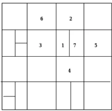
-torus.2 This coordinate space is completelylogical and bears no relation to any physical coordinate system. At any point in time, the entire coordinate space is dynamically par-titioned among all the nodes in the system such that every node “owns” its individual, distinct zone within the overall space. For example, Figure 1 shows a 2-dimensional[0
;
1][0;
1]coordinatespace partitioned between 5 CAN nodes.
This virtual coordinate space is used to store (key,value) pairs as follows: to store a pair (
K
1,V
1), keyK
1 is deterministicallymapped onto a point
P
in the coordinate space using a uniform hash function. The corresponding (key,value) pair is then stored at the node that owns the zone within which the pointP
lies. To retrieve an entry corresponding to keyK
1, any node can apply thesame deterministic hash function to map
K
1onto pointP
and thenretrieve the corresponding value from the point
P
. If the pointP
is not owned by the requesting node or its immediate neighbors, the request must be routed through the CAN infrastructure until it reaches the node in whose zoneP
lies. Efficient routing is therefore a critical aspect of a CAN.Nodes in the CAN self-organize into an overlay network that rep-resents this virtual coordinate space. A node learns and maintains the IP addresses of those nodes that hold coordinate zones adjoin-ing its own zone. This set of immediate neighbors in the coordinate space serves as a coordinate routing table that enables routing be-tween arbitrary points in this space.
We will describe the three most basic pieces of our design: CAN routing, construction of the CAN coordinate overlay, and mainte-nance of the CAN overlay.
2.1
Routing in a CAN
2For simplicity, the illustrations in this paper do not show a torus, so the reader must remember that the coordinate space wraps.
Intuitively, routing in a Content Addressable Network works by following the straight line path through the Cartesian space from source to destination coordinates.
A CAN node maintains a coordinate routing table that holds the IP address and virtual coordinate zone of each of its immediate neighbors in the coordinate space. In a
d
-dimensional coordinate space, two nodes are neighbors if their coordinate spans overlap alongd
;1dimensions and abut along one dimension. For example,in Figure 2, node 5 is a neighbor of node 1 because its coordinate zone overlaps with 1’s along the Y axis and abuts along the X-axis. On the other hand, node 6 is not a neighbor of 1 because their co-ordinate zones abut along both the X and Y axes. This purely local neighbor state is sufficient to route between two arbitrary points in the space: A CAN message includes the destination coordinates. Using its neighbor coordinate set, a node routes a message towards its destination by simple greedy forwarding to the neighbor with coordinates closest to the destination coordinates. Figure 2 shows a sample routing path.
For a
d
dimensional space partitioned inton
equal zones, the av-erage routing path length is(d=
4)(n
1=d
)hops and individual nodes
maintain2
d
neighbors3. These scaling results mean that for a
d
-dimensional space, we can grow the number of nodes (and hence zones) without increasing per node state while the average path length grows as
O
(n
1=d ).
Note that many different paths exist between two points in the space and so, even if one or more of a node’s neighbors were to crash, a node can automatically route along the next best available path.
If however, a node loses all its neighbors in a certain direction, and the repair mechanisms described in Section 2.3 have not yet rebuilt the void in the coordinate space, then greedy forwarding may temporarily fail. In this case, a node may use an expanding ring search (using stateless, controlled flooding over the unicast CAN overlay mesh) to locate a node that is closer to the destination than itself. The message is then forwarded to this closer node, from which greedy forwarding is resumed.
2.2
CAN construction
As described above, the entire CAN space is divided amongst the nodes currently in the system. To allow the CAN to grow in-crementally, a new node that joins the system must be allocated its own portion of the coordinate space. This is done by an existing node splitting its allocated zone in half, retaining half and handing the other half to the new node.
The process takes three steps:
1. First the new node must find a node already in the CAN. 2. Next, using the CAN routing mechanisms, it must find a node
whose zone will be split.
3. Finally, the neighbors of the split zone must be notified so that routing can include the new node.
Bootstrap
A new CAN node first discovers the IP address of any node cur-rently in the system. The functioning of a CAN does not depend
3
Recently proposed routing algorithms for location services [15, 20] route in
O
(logn
)hops with each node maintainingO
(logn
)neighbors. Notice that were we to select the number of dimensions
d=(log
2
n
)
=
2, we could achieve the same scaling properties.Wechoose to hold d fixed independent of n, since we envision apply-ing CANs to very large systems with frequent topology changes. In such systems, it is important to keep the number of neighbors independent of the system size
node B’s virtual coordinate zone (0.5-1.0,0.0-0.5)
(0-0.5,0-0.5) (0-0.5,0.5-1.0)
(0.75-1.0,0.5-1.0) 1.0
0.0 1.0
0.0
A B
D E
C
(0.5-0.75,0.5-1.0)
Figure 1: Example 2-d space with 5 nodes
7’s coordinate neighbor set = { }
1 5
2
3 6
4
(x,y)
sample routing path from node 1 to point (x,y)
1’s coordinate neighbor set = {2,3,4,5}
Figure 2: Example 2-d space before node
7 joins
7 5
2
3
4 6
1’s coordinate neighbor set = {2,3,4,7} 7’s coordinate neighbor set = {1,2,4,5}
1
Figure 3: Example 2-d space after node
7 joins
on the details of how this is done, but we use the same bootstrap mechanism as YOID [4].
As in [4] we assume that a CAN has an associated DNS domain name, and that this resolves to the IP address of one or more CAN bootstrap nodes. A bootstrap node maintains a partial list of CAN nodes it believes are currently in the system. Simple techniques to keep this list reasonably current are described in [4].
To join a CAN, a new node looks up the CAN domain name in DNS to retrieve a bootstrap node’s IP address. The bootstrap node then supplies the IP addresses of several randomly chosen nodes currently in the system.
Finding a Zone
The new node then randomly chooses a point
P
in the space and sends aJOINrequest destined for pointP
. This message is sent into the CAN via any existing CAN node. Each CAN node then uses the CAN routing mechanism to forward the message, until it reaches the node in whose zoneP
lies.This current occupant node then splits its zone in half and assigns one half to the new node. The split is done by assuming a certain ordering of the dimensions in deciding along which dimension a zone is to be split, so that zones can be re-merged when nodes leave. For a 2-d space a zone would first be split along the X dimension, then the Y and so on. The (key, value) pairs from the half zone to be handed over are also transfered to the new node.
Joining the Routing
Having obtained its zone, the new node learns the IP addresses of its coordinate neighbor set from the previous occupant. This set is a subset of the previous occupant’s neighbors, plus that occupant itself. Similarly, the previous occupant updates its neighbor set to eliminate those nodes that are no longer neighbors. Finally, both the new and old nodes’ neighbors must be informed of this realloca-tion of space. Every node in the system sends an immediate update message, followed by periodic refreshes, with its currently assigned zone to all its neighbors. These soft-state style updates ensure that all of their neighbors will quickly learn about the change and will update their own neighbor sets accordingly. Figures 2 and 3 show an example of a new node (node 7) joining a 2-dimensional CAN.
The addition of a new node affects only a small number of ex-isting nodes in a very small locality of the coordinate space. The number of neighbors a node maintains depends only on the dimen-sionality of the coordinate space and is independent of the total
number of nodes in the system. Thus, node insertion affects only
O(number of dimensions) existing nodes, which is important for
CANs with huge numbers of nodes.
2.3
Node departure, recovery and CAN
main-tenance
When nodes leave a CAN, we need to ensure that the zones they occupied are taken over by the remaining nodes. The normal pro-cedure for doing this is for a node to explicitly hand over its zone and the associated (key,value) database to one of its neighbors. If the zone of one of the neighbors can be merged with the departing node’s zone to produce a valid single zone, then this is done. If not, then the zone is handed to the neighbor whose current zone is smallest, and that node will then temporarily handle both zones.
The CAN also needs to be robust to node or network failures, where one or more nodes simply become unreachable. This is han-dled through an immediate takeover algorithm that ensures one of the failed node’s neighbors takes over the zone. However in this case the (key,value) pairs held by the departing node are lost until the state is refreshed by the holders of the data4.
Under normal conditions a node sends periodic update messages to each of its neighbors giving its zone coordinates and a list of its neighbors and their zone coordinates. The prolonged absence of an update message from a neighbor signals its failure.
Once a node has decided that its neighbor has died it initiates the takeover mechanism and starts a takeover timer running. Each neighbor of the failed node will do this independently, with the timer initialized in proportion to the volume of the node’s own zone. When the timer expires, a node sends aTAKEOVERmessage conveying its own zone volume to all of the failed node’s neighbors. On receipt of aTAKEOVER message, a node cancels its own timer if the zone volume in the message is smaller that its own zone volume, or it replies with its ownTAKEOVERmessage. In this way, a neighboring node is efficiently chosen that is still alive and has a small zone volume5.
Under certain failure scenarios involving the simultaneous fail-ure of multiple adjacent nodes, it is possible that a node detects
4
To prevent stale entries as well as to refresh lost entries, nodes that insert (key,value) pairs into the CAN periodically refresh these entries
5
Additional metrics such as load or the quality of connectivity can also be taken into account, but in the interests of simplicity we won’t discuss these further here.
a failure, but less than half of the failed node’s neighbors are still reachable. If the node takes over another zone under these circum-stances, it is possible for the CAN state to become inconsistent. In such cases, prior to triggering the repair mechanism, the node per-forms an expanding ring search for any nodes residing beyond the failure region and hence it eventually rebuilds sufficient neighbor state to initiate a takeover safely.
Finally, both the normal leaving procedure and the immediate takeover algorithm can result in a node holding more than one zone. To prevent repeated further fragmentation of the space, a background zone-reassignment algorithm, which we describe in Appendix A, runs to ensure that the CAN tends back towards one zone per node.
3.
DESIGN IMPROVEMENTS
Our basic CAN algorithm as described in the previous section provides a balance between low per-node state (
O
(d
) for ad
-dimensional space) and short path lengths withO
(dn
1=d)hops
for
d
dimensions andn
nodes. This bound applies to the number of hops in the CAN path. These are application level hops, not IP-level hops, and the latency of each hop might be substantial; recall that nodes that are adjacent in the CAN might be many miles and many IP hops away from each other. The average total latency of a lookup is the average number of CAN hops times the average la-tency of each CAN hop. We would like to achieve a lookup lala-tency that is comparable within a small factor to the underlying IP path latencies between the requester and the CAN node holding the key. In this section, we describe a number of design techniques whose primary goal is to reduce the latency of CAN routing. Not unin-tentionally, many of these techniques offer the additional advan-tage of improved CAN robustness both in terms of routing and data availability. In a nutshell, our strategy in attempting to reduce path latency is to reduce either the path length or the per-CAN-hop la-tency. A final improvement we make to our basic design is to add simple load balancing mechanisms (described in Sections 3.7 and 3.8).First, we describe and evaluate each design feature individually and then, in Section 4, discuss how together they affect the overall performance. These added features yield significant improvements but come at the cost of increased per-node state (although per-node state still remains independent of the number of nodes in the sys-tem) and somewhat increased complexity. The extent to which the following techniques are applied (if at all) involves a trade-off be-tween improved routing performance and system robustness on the one hand and increased per-node state and system complexity on the other. Until we have greater deployment experience, and know the application requirements better, we are not prepared to decide on these tradeoffs.
We simulated our CAN design on Transit-Stub (TS) topologies using the GT-ITM topology generator [22]. TS topologies model networks using a 2-level hierarchy of routing domains with transit domains that interconnect lower level stub domains.
3.1
Multi-dimensioned coordinate spaces
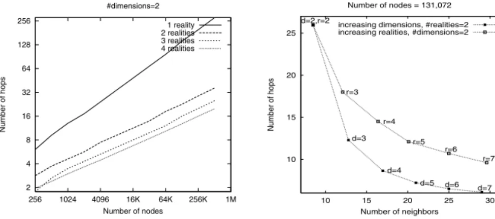
The first observation is that our design does not restrict the di-mensionality of the coordinate space. Increasing the dimensions of the CAN coordinate space reduces the routing path length, and hence the path latency, for a small increase in the size of the coor-dinate routing table.
Figure 4 measures this effect of increasing dimensions on rout-ing path length. We plot the path length for increasrout-ing numbers of CAN nodes for coordinate spaces with different dimensions. For a system with
n
nodes andd
dimensions, we see that the path lengthscales as
O
(d
(n
1=d))in keeping with the analytical results for
per-fectly partitioned coordinate spaces.
Because increasing the number of dimensions implies that a node has more neighbors, the routing fault tolerance also improves as a node now has more potential next hop nodes along which messages can be routed in the event that one or more neighboring nodes crash.
3.2
Realities: multiple coordinate spaces
The second observation is that we can maintain multiple, inde-pendent coordinate spaces with each node in the system being as-signed a different zone in each coordinate space. We call each such coordinate space a “reality”. Hence, for a CAN with
r
realities, a single node is assignedr
coordinate zones, one on every reality and holdsr
independent neighbor sets.The contents of the hash table are replicated on every reality. This replication improves data availability. For example, say a pointer to a particular file is to be stored at the coordinate loca-tion (x,y,z). With four independent realities, this pointer would be stored at four different nodes corresponding to the coordinates (x,y,z) on each reality and hence it is unavailable only when all four nodes are unavailable. Multiple realities also improve rout-ing fault tolerance, because in the case of a routrout-ing breakdown on one reality, messages can continue to be routed using the remaining realities.
Further, because the contents of the hash table are replicated on every reality, routing to location (x,y,z) translates to reaching (x,y,z) on any reality. A given node owns one zone per reality each of which is at a distinct, and possibly distant, location in the coordi-nate space. Thus, an individual node has the ability to reach distant portions of the coordinate space in a single hop, thereby greatly re-ducing the average path length. To forward a message, a node now checks all its neighbors on each reality and forwards the message to that neighbor with coordinates closest to the destination. Figure 5 plots the path length for increasing numbers of nodes for different numbers of realities. From the graph, we see that realities greatly reduce path length. Thus, using multiple realities reduces the path length and hence the overall CAN path latency.
Multiple dimensions versus multiple realities
Increasing either the number of dimensions or realities results in shorter path lengths, but higher per-node neighbor state and main-tenance traffic. Here we compare the relative improvements caused by each of these features.
Figure 6 plots the path length versus the average number of neigh-bors maintained per node for increasing dimensions and realities. We see that for the same number of neighbors, increasing the di-mensions of the space yields shorter path lengths than increasing the number of realities. One should not, however, conclude from these tests that multiple dimensions are more valuable than multi-ple realities because multimulti-ple realities offer other benefits such as improved data availability and fault-tolerance. Rather, the point to take away is that if one were willing to incur an increase in the av-erage per-node neighbor state for the primary purpose of improving routing efficiency, then the right way to do so would be to increase the dimensionality
d
of the coordinate space rather than the number of realitiesr
.3.3
Better CAN routing metrics
The routing metric, as described in Section 2.1, is the progress in terms of Cartesian distance made towards the destination. One can improve this metric to better reflect the underlying IP topology by having each node measure the network-level round-trip-time
4 8 16 32 64 128 256
256 1024 4096 16K 64K 256K 1M
Number of hops
Number of nodes #realities=1
2 dimensions 3 dimensions 4 dimensions 5 dimensions
Figure 4: Effect of dimensions on path
length
2 4 8 16 32 64 128 256
256 1024 4096 16K 64K 256K 1M
Number of hops
Number of nodes #dimensions=2
1 reality 2 realities 3 realities 4 realities
Figure 5: Effect of multiple realities on
path length
10 15 20 25
10 15 20 25 30
Number of hops
Number of neighbors Number of nodes = 131,072 d=2,r=2
d=3 d=4
d=5 d=6 d=7 r=3
r=4 r=5
r=6 r=7 increasing dimensions, #realities=2 increasing realities, #dimensions=2
Figure 6: Path length with increasing
neighbor state
is forwarded to the neighbor with the maximum ratio of progress to RTT. This favors lower latency paths, and helps the application level CAN routing avoid unnecessarily long hops.
Unlike increasing the number of dimensions or realities, RTT-weighted routing aims at reducing the latency of individual hops along the path and not at reducing the path length. Thus, our metric for evaluating the efficacy of RTT-weighted routing is the per-hop latency, obtained by dividing the overall path latency by the path length.
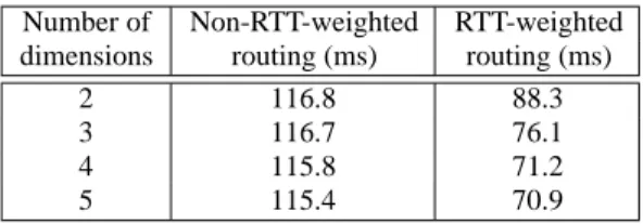
To quantify the effect of this routing metric, we used Transit-Stub topologies with link latencies of 100ms for intra-transit main links, 10ms for stub-transit links and 1ms for intra-stub do-main links. With our simulated topology, the average end-to-end la-tency of the underlying IP network path between randomly selected source-destination nodes is approximately 115ms. Table 1 com-pares the average per-hop latency with and without RTT weighting. These latencies were averaged over test runs with
n
, the number of nodes in the CAN, ranging from28
to2 18
.
As can be seen, while the per-hop latency without RTT-weighted routing matches the underlying average IP network latency, RTT-weighted routing lowers the per-hop latency by between 24% and 40% depending on the number of dimensions. Higher dimensions give more next-hop forwarding choices and hence even greater im-provements.
3.4
Overloading coordinate zones
So far, our design assumes that a zone is, at any point in time, assigned to a single node in the system. We now modify this to allow multiple nodes to share the same zone. Nodes that share the same zone are termed peers. We define a system parameter
MAXPEERS, which is the maximum number of allowable peers per
zone (we imagine that this value would typically be rather low, 3 or 4 for example).
With zone overloading, a node maintains a list of its peers in ad-dition to its neighbor list. While a node must know all the peers in its own zone, it need not track all the peers in its neighboring zones. Rather, a node selects one neighbor from amongst the peers in each of its neighboring zones. Thus, zone overloading does not increase the amount of neighbor information an individual node must hold, but does require it to hold additional state for up toMAXPEERS
peer nodes.
Overloading a zone is achieved as follows: When a new node
A
joins the system, it discovers, as before, an existent nodeB
whose zone it is meant to occupy. Rather than directly splitting its zoneas described earlier, node
B
first checks whether it has fewer thanMAXPEERSpeer nodes. If so, the new node
A
merely joinsB
’szone without any space splitting. Node
A
obtains both its peer list and its list of coordinate neighbors fromB
. Periodic soft-state updates fromA
serve to informA
’s peers and neighbors about its entry into the system.If the zone is full (already hasMAXPEERSnodes), then the zone is split into half as before. Node
B
informs each of the nodes on it’s peer-list that the space is to be split. Using a deterministic rule (for example the ordering of IP addresses), the nodes on the peer list together with the new nodeA
divide themselves equally between the two halves of the now split zone. As before,A
obtains its initial list of peers and neighbors fromB
.Periodically, a node sends its coordinate neighbor a request for its list of peers, then measures the RTT to all the nodes in that neighboring zone and retains the node with the lowest RTT as its neighbor in that zone. Thus a node will, over time, measure the round-trip-time to all the nodes in each neighboring zone and retain the closest (i.e. lowest latency) nodes in its coordinate neighbor set. After its initial bootstrap into the system, a node can perform this RTT measurement operation at very infrequent intervals so as to not unnecessarily generate large amounts of control traffic.
The contents of the hash table itself may be either divided or replicated across the nodes in a zone. Replication provides higher availability but increases the size of the data stored at every node by a factor ofMAXPEERS(because the overall space is now partitioned into fewer, and hence larger, zones) and data consistency must be maintained across peer nodes. On the other hand, partitioning data among a set of peer nodes does not require consistency mechanisms or increased data storage but does not improve availability either.
Overloading zones offers many advantages:
reduced path length (number of hops), and hence reduced
path latency, because placing multiple nodes per zone has the same effect as reducing the number of nodes in the system.
reduced per-hop latency because a node now has multiple
choices in its selection of neighboring nodes and can select neighbors that are closer in terms of latency. Table 2 lists the average per-hop latency for increasingMAXPEERSfor system sizes ranging from 2
8
to2 18
nodes with the same Transit-Stub simulation topologies as in Section 3.3. We see that placing 4 nodes per zone can reduce the per-hop latency by about 45%.
Number of Non-RTT-weighted RTT-weighted dimensions routing (ms) routing (ms)
2 116.8 88.3
3 116.7 76.1
4 115.8 71.2
5 115.4 70.9
Table 1: Per-hop latency using RTT-weighted routing
Number of nodes per zone per-hop latency (ms)
1 116.4
2 92.8
3 72.9
4 64.4
Table 2: Per-hop latencies using multiple nodes per zone
all the nodes in a zone crash simultaneously (in which case
the repair process of Section 2.3 is still required).
On the negative side, overloading zones adds somewhat to sys-tem complexity because nodes must additionally track a set of peers.
3.5
Multiple hash functions
For improved data availability, one could use
k
different hash functions to map a single key ontok
points in the coordinate space and accordingly replicate a single (key,value) pair atk
distinct nodes in the system. A (key,value) pair is then unavailable only when allk
replicas are simultaneously unavailable. In addition, queries for a particular hash table entry could be sent to allk
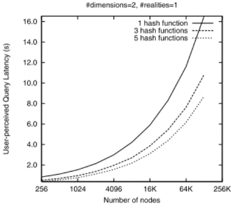
nodes in paral-lel thereby reducing the average query latency. Figure 7 plots this query latency, i.e. the time to fetch a (key,value) pair, for increasing number of nodes for different numbers of hash functions.Of course, these advantages come at the cost of increasing the size of the (key,value) database and query traffic (in the case of parallel queries) by a factor of
k
.Instead of querying all
k
nodes, a node might instead choose to retrieve an entry from that node which is closest to it in the coordi-nate space.3.6
Topologically-sensitive construction of the
CAN overlay network
The CAN construction mechanism described in Section 2.2 allo-cates nodes to zones at random, and so a node’s neighbors on the CAN need not be topologically nearby on the underlying IP net-work. This can lead to seemingly strange routing scenarios where, for example, a CAN node in Berkeley has its neighbor nodes in Eu-rope and hence its path to a node in nearby Stanford may traverse distant nodes in Europe. While the design mechanisms described in the previous sections try to improve the selection of paths on an existing overlay network they do not try to improve the overlay net-work structure itself. In this section, we present some initial results on our current work on trying to construct CAN topologies that are congruent with the underlying IP topology.
Our initial scheme assumes the existence of a well known set of machines (for example, the DNS root name servers) that act as landmarks on the Internet. We achieve a form of “distributed bin-ning” of CAN nodes based on their relative distances from this set of landmarks. Every CAN node measures its round-trip-time to each of these landmarks and orders the landmarks in order of in-creasing RTT. Thus, based on its delay measurements to the differ-ent landmarks, every CAN node has an associated ordering. With
m
landmarks,m
!such orderings are possible. Accordingly wepartition the coordinate space into
m
!equal sized portions, eachcorresponding to a single ordering. Our current (somewhat naive) scheme to partition the space into
m
!portions works as follows:as-suming a fixed cyclical ordering of the dimensions (e.g. xyzxyzx...), we first divide the space, along the first dimension, into
m
portions, each portion is then sub-divided along the second dimension intom
;1portions each of which is further divided intom
;2por-tions and so on. Previously, a new node joined the CAN at a ran-dom point in the entire coordinate space. Now, a new node joins the CAN at a random point in that portion of the coordinate space associated with its landmark ordering.
The rationale behind this scheme is that topologically close nodes are likely to have the same ordering and consequently, will reside in the same portion of the coordinate space and hence neighbors in the coordinate space are likely to be topologically close on the Internet.
The metric we use to evaluate the above binning scheme is the ratio of the latency on the CAN network to the average latency on the IP network. We call this the latency stretch. Figure 8 compares the stretch on CANs constructed with and without the above land-mark ordering scheme. We use the same Transit-Stub topologies as before (Section 3.3) and 4 landmarks placed at random with the only restriction that they must be at least 5 hops away from each other. As can be seen, landmark ordering greatly improves the path latency.
A consequence of the above binning strategy is that the coordi-nate space is no longer uniformly populated. Because some order-ings (bins) are more likely to occur than others their corresponding portions of the coordinate space are also more densely occupied than others leading to a slightly uneven distribution of load amongst the nodes. The use of background load balancing techniques (as described in Appendix A) where an overloaded node hands off a portion of its space to a more lightly loaded one could be used to alleviate this problem.
These results seem encouraging and we are continuing to study the effect of topology, link delay distribution, number of landmarks and other factors on the above scheme. Landmark ordering is work in progress. We do not discuss or make use of it further in this paper.
3.7
More Uniform Partitioning
When a new node joins, a JOIN message is sent to the owner of a random point in the space. This existing node knows not only its own zone coordinates, but also those of its neighbors. Therefore, instead of directly splitting its own zone, the existing occupant node first compares the volume of its zone with those of its immediate neighbors in the coordinate space. The zone that is split to accom-modate the new node is then the one with the largest volume.
This volume balancing check thus tries to achieve a more uni-form partitioning of the space over all the nodes and can be used with or without the landmark ordering scheme from Section 3.6. Since (key,value) pairs are spread across the coordinate space using a uniform hash function, the volume of a node’s zone is indicative of the size of the (key,value) database the node will have to store, and hence indicative of the load placed on the node. A uniform par-titioning of the space is thus desirable to achieve load balancing.
Note that this is not sufficient for true load balancing because some (key,value) pairs will be more popular than others thus putting higher load on the nodes hosting those pairs. This is similar to the
2.0 4.0 6.0 8.0 10.0 12.0 14.0 16.0
256 1024 4096 16K 64K 256K
User-perceived Query Latency (s)
Number of nodes #dimensions=2, #realities=1
1 hash function 3 hash functions 5 hash functions
Figure 7: Reduction in user-perceived
query latency with the use of multiple hash functions
0 5 10 15 20 25
256 1024 4096
Latency Stretch
Number of nodes #landmarks=4, #realities=1
2-d, with landmark ordering 2-d, without landmark ordering 4-d, with landmark ordering 4-d, without landmark ordering
Figure 8: Latency savings due to
land-mark ordering used in CAN construction
0 20 40 60 80 100
V/16 V/8 V/4 V/2 V 2V 4V 8V
Percentage of nodes
Volume
without uniform-partitioning feature with uniform-partitioning feature
Figure 9: Effect of Uniform Partitioning
feature on a CAN with 65,536 nodes, 3 dimensions and 1 reality
“hot spot” problem on the Web. In Section 3.8 we discuss caching and replication techniques that can be used to ease this hot spot problem in CANs.
If the total volume of the entire coordinate space were
V
T andn
the total number of nodes in the system then a perfect partitioning of the space among the
n
nodes would assign a zone of volumeV
T/n
to each node. We useV
to denoteV
T/n
. We ran simulationswith2 16
nodes both with and without this uniform partitioning fea-ture. At the end of each run, we compute the volume of the zone assigned to each node. Figure 9 plots different possible volumes in terms of
V
on the X axis and shows the percentage of the total number of nodes (Y axis) that were assigned zones of a particular volume. From the plot, we can see that without the uniform parti-tioning feature a little over 40% of the nodes are assigned to zones with volumeV
as compared to almost 90% with this feature and the largest zone volume drops from8V
to2V
. Not surprisingly,the partitioning of the space further improves with increasing di-mensions.
3.8
Caching and Replication techniques for
“hot spot” management
As with files in the Web, certain (key,value) pairs in a CAN are likely to be far more frequently accessed than others, thus overload-ing nodes that hold these popular data keys. To make very popular data keys widely available, we borrow some of the caching and replication techniques commonly applied to the Web.
Caching: In addition to its primary data store (i.e. those data
keys that hash into its coordinate zone), a CAN node main-tains a cache of the data keys it recently accessed. Before forwarding a request for a data key towards its destination, a node first checks whether the requested data key is in its own cache and if so, can itself satisfy the request without forwarding it any further. Thus, the number of caches from which a data key can be served grows in direct proportion to its popularity and the very act of requesting a data key makes it more widely available.
Replication: A node that finds it is being overloaded by
re-quests for a particular data key can replicate the data key at each of its neighboring nodes. Replication is thus an ac-tive pushing out of popular data keys as opposed to caching, which is a natural consequence of requesting a data key. A
popular data key is thus eventually replicated within a re-gion surrounding the original storage node. A node holding a replica of a requested data key can, with a certain prob-ability, choose to either satisfy the request or forward it on its way thereby causing the load to be spread over the entire region rather than just along the periphery.
As with all such schemes, cached and replicated data keys should have an associated time-to-live field and be eventually expired from the cache.
4.
DESIGN REVIEW
Sections 2 and 3 described and evaluated individual CAN design components. The evaluation of our CAN recovery algorithms (us-ing both large scale and smaller scale ns simulations), are presented in [18]. Here we briefly recap our design parameters and metrics, summarize the effect of each parameter on the different metrics and quantify the performance gains achieved by the cumulative effect of all the features.
We used the following metrics to evaluate system performance:
Path length: the number of (application-level) hops required
to route between two points in the coordinate space.
Neighbor-state: the number of CAN nodes for which an
in-dividual node must retain state.
Latency: we consider both the end-end latency of the
to-tal routing path between two points in the coordinate space and the per-hop latency, i.e., latency of individual application level hops obtained by dividing the end-to-end latency by the path length.
Volume: the volume of the zone to which a node is assigned,
that is indicative of the request and storage load a node must handle.
Routing fault tolerance: the availability of multiple paths
between two points in the CAN.
Hash table availability: adequate replication of a (key,value)
entry to withstand the loss of one or more replicas. The key design parameters affecting system performance are:
dimensionality of the virtual coordinate space: d number of realities: r
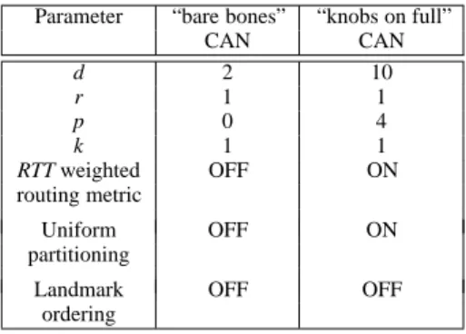
Parameter “bare bones” “knobs on full”
CAN CAN
d 2 10
r 1 1
p 0 4
k 1 1
RTT weighted OFF ON routing metric
Uniform OFF ON
partitioning
Landmark OFF OFF
ordering
Table 4: CAN parameters
Metric “bare bones” CAN “knobs on full CAN” path length 198.0 5.0 # neighbors 4.57 27.1
# peers 0 2.95
IP latency 115.9ms 82.4ms CAN path latency 23,008ms 135.29ms
Table 5: CAN Performance Results
number of hash functions (i.e. number of points per reality
at which a (key,value) pair is stored): k
use of the RTT-weighted routing metric
use of the uniform partitioning feature described in Section 3.7
In some cases, the effect of a design parameter on certain met-rics can be directly inferred from the algorithm; in all other cases we resorted to simulation. Table 3 summarizes the relationship be-tween the different parameters and metrics. A table entry marked “-” indicates that the given parameter has no significant effect on that metric, while"and#indicate an increase and decrease
respec-tively in that measure caused by an increase in the corresponding parameter. The figure numbers included in certain table entries re-fer to the corresponding simulation results.
To measure the cumulative effect of all the above features, we se-lected a system size of n=2
18
nodes and compared two algorithms: 1. a “bare bones” CAN that does not utilize most of our
addi-tional design features
2. a “knobs-on-full” CAN making full use of our added features (without the landmark ordering feature from Section 3.7) The topology used for this test is a Transit-Stub topology with a delay of 100ms on intra-transit links, 10ms on stub-transit links and 1ms on intra-stub links (i.e. 100ms on links that connect two transit nodes, 10ms on links that connect a transit node to a stub node and so forth). Tables 4 and 5 list the values of the parameters and metrics for each test.6
We find these results encouraging as they demonstrate that for a system with over 260,000 nodes we can route with a latency that is well within a factor of two of the underlying network latency. The number of neighbors that a node must maintain to achieve this is approximately 30 (27.1 + 2.95) which is definitely on the high side but not necessarily unreasonable. The biggest gain comes from increasing the number of dimensions, which lowers the path length from 198 to approximately 5 hops. However, we can see that the latency reduction heuristics play an important role; without latency heuristics, the end-to-end latency would be close to5115ms (#
hops# latency-per-hop).
We repeated the above “knobs-on-full” simulation and varied the system size n from2
14
to2 18
. In scaling the CAN system, we scaled the topology by scaling the number of CAN nodes added
6
The reason the IP latency is 82ms (in the “knobs-on-full” test) instead of 115ms is not because the average latency of the physical network is lower but because our CAN algorithm (because of the use of zone overloading and RTT-weighted routing) automatically retrieves an entry from the closest replica. 82ms represents the average IP network level latency from the retrieving node to this closest replica.
1.4 1.6 1.8 2 2.2 2.4 2.6 2.8 3 3.2
16K 32K 65K 131K
Latency Stretch
Number of nodes H(100,10,1)
H(20,5,2) R(10,50) 10xH(20,5,2)
Figure 10: Effect of link delay distribution on CAN latency
to the edges of the topology without scaling the backbone topol-ogy itself. This effectively grows the density at the edges of the topology. We found, that as n grows, the total path latency grows even more slowly than
n
1=d(with
d
=10in this case) becauseal-though the path length grows slowly as
n
1=10(from 4.56 hops with
2 14
nodes to 5.0 with2 18
hops) the latency of the additional hops is lower than the average latency since the added hops are along low-latency links at the edges of the network.
Extrapolating this scaling trend and making the pessimistic as-sumption that the total latency grows with the increase in path length (i.e., as
n
1=10) we could potentially scale the size of the system by another2
10
, reaching a system size of close to a billion nodes, before seeing the path latency increase to within a factor of four of the underlying network latency.
To better understand the effect of link delay distributions on the above results, we repeated the “knobs-on-full” test for different de-lay distributions on the Transit-Stub topologies. We used the fol-lowing topologies:
H
(100;
10;
1): A Transit-Stub topology with a hierarchicallink delay assignment of 100ms on intra-transit links, 10ms on transit-stub links and 1ms on intra-stub links. This is the topology used in the above “knobs-on-full” test.
H
(20;
5;
2): A Transit-Stub topology with a hierarchical linkdelay assignment of 20ms on intra-transit links, 5ms on transit-stub links and 2ms on intra-transit-stub links.
Design P arameters path length (hops) neighbor state total path latenc y per -hop la-tenc y size of data store routing fault toler -ance data store av ailability dimensions: d
O
(dn
1 =d ) (fig: 4)O
(d
) # (due to reduced path length) -" -realities: r # (fig: 5)O
(r
) # (due to reduced path length)-O
(r
) "O
(r
) number of peer nodes per zone: pO
(1=p
)O
(p
) # (due to reduced path length and reduced per -hop latenc y) # (table: 2) replicated data store repli-cated:O
(p
) , partitioned data store: -" (due to backup neighbors) replicated data store:O
(p
) , partitioned data store: -number of hash functions: k -# (fig: 7)-O
(k
)-O
(k
) use of R T T -weighted routing metric -# (due to reduced per -hop latenc y) # (table: 1) -use of uniform partitioning feature reduced v ariance reduced v ariance -reduced v ariance (fig: 9) -T able 3: Ef fect of design parameters on perf ormance metrics
R
(10;
50): A Transit-Stub topology with the delay of everylink set to a random value between 10ms to 50ms.
10
xH
(20;
5;
2): This topology is the same asH
(20;
5;
2)except that the backbone topology is scaled by a factor of 10 which implies that the density of CAN nodes on the resultant topology is about 10 times lower.
For each of the above topologies, we measure the latency stretch - the ratio of CAN latency to IP latency - for different system sizes. The results are shown in Figure 10. We see that while the delay distribution affects the absolute value of the latency stretch, in all cases, the latency stretch grows very slowly with system size. In no case do we see a latency stretch of more than 3 for system sizes up to 130,000 nodes. The fastest growth is in the case of random delay distributions. This is because in this case, as we grow the CAN system size, the new links added at the edges of the network need not be low latency links (unlike with the hierarchical delay distributions). Finally, we see that latency stretch with topology
H
(20;
5;
2)is slightly lower than with topology10xH
(20;
5;
2).This is due to the higher density of CAN nodes in the case of
H
(20;
5;
2); higher densities allow the latency heuristics to yieldhigher gains.
5.
RELATED WORK
We categorize related work as related algorithms in the litera-ture relevant to data location and related systems that involve a data location component.
5.1
Related Algorithms
The Distance Vector (DV) and Link State (LS) algorithms used in IP routing require every router to have some level of knowledge (the exact link structure in the case of LS and the distance in hops for DV) of the topology of entire network. Unlike our CAN routing algorithm, DV and LS thus require the widespread dissemination of local topology information. While well suited to IP networks wherein topology changes are infrequent, for networks with fre-quent topology changes, DV and LS would result in the frefre-quent propagation of routing updates. Because we wanted our CAN de-sign to scale to large numbers of potentially flaky nodes we chose not to use routing schemes such as DV and LS.
Another goal in designing CANs was to have a truly distributed routing algorithm, both because this does not stress a small set of nodes and because it avoids a single point of failure. Hence we avoided more traditional hierarchical routing algorithms [16, 19, 11, 3].
Perhaps closest in spirit to the CAN routing scheme is the Plax-ton algorithm [15]. In PlaxPlax-ton’s algorithm, every node is assigned a unique n bit label. This
n
bit label is divided into l levels, with each level havingw
=n=l
bits. A node with label, sayxyz
, wherex,y and z are
w
bit digits, will have a routing table with:2 w
entries of the form:
X X
2w
entries of the form:
x
X
2w
entries of the form:
x y
where we use the notationto denote every digit in0
;:::;
2 w;1,
and
X
to denote any digit in0;:::;
2 w;1.
Using the above routing state, a packet is forwarded towards a destination label node by incrementally “resolving” the destination label from left to right, i.e., each node forwards a packet to a neigh-bor whose label matches (from left to right) the destination label in one more digit than its own label does.
For a system with
n
nodes, Plaxton’s algorithm routes inO
(logn
)hops and requires a routing table size that is
O
(logn
). CANrout-ing by comparison routes in
O
(dn
1=d)hops (where
d
isdimen-sions) with routing table size
O
(dr
)which is independent ofn
. Asmentioned earlier, setting
d
=(log 2n
)
=
2allows our CANalgo-rithm to match Plaxton’s scaling properties. Plaxton’s algoalgo-rithm addresses many of the same issues we do. As such it was a natural candidate for CANs and, early into our work, we seriously consid-ered using it. However, on studying the details of the algorithm, we decided that it was not well-suited to our application. This is primarily because the Plaxton algorithm was originally proposed for web caching environments which are typically administratively configured, have fairly stable hosts and maximal scales on the or-der of thousands. While the Plaxton algorithm is very well suited to such environments, the peer-to-peer contexts we address are quite different. We require a self-configuring system which is capable of dealing with a very large set of hosts (millions), many of them potentially quite flaky. However, because the targeted application is web caching, the Plaxton algorithm does not provide a solution whereby nodes can independently discover their neighbors in a de-centralized manner. In fact, the algorithm requires global knowl-edge of the topology to achieve a consistent mapping between data objects and the Plaxton nodes holding those objects. Addition-ally, every node arrival and departure affects a logarithmic number of nodes which, for large systems with high arrival and departure rates, appears to be on the high side because nodes could be con-stantly reacting to changes in system membership.
Algorithms built around the concept of geographic routing [9, 12] are similar to our CAN routing algorithm in that they build around the notion of forwarding messages through a coordinate space. The key difference is that the “space” in their work refers to true physical space because of which there is no neighbor dis-covery problem (i.e. a node’s neighbors are those that lie in its ra-dio range). These algorithms are very well suited to their targeted applications of routing and location services in ad-hoc networks. Applying such algorithms to our CAN problem would require us to construct and maintain neighbor relationships that would correctly mimic geographic space which appears non trivial (for example, GPSR performs certain planarity checks which would be hard to achieve without a physical radio medium). Additionally, such ge-ographic routing algorithms are not obviously extensible to multi-dimensional spaces.
5.2
Related Systems
5.2.1
Domain Name System
The DNS system in some sense provides the same functionality as a hash table; it stores key value pairs of the form (domain name, IP address). While a CAN could potentially provide a distributed DNS-like service, the two systems are quite different. In terms of functionality, CANs are more general than the DNS. The current design of the DNS closely ties the naming scheme to the manner in which a name is resolved to an IP address, CAN name resolution is truly independent of the naming scheme. In terms of design, the two systems are very different.
5.2.2
OceanStore
The OceanStore project at U.C.Berkeley [10] is building a utility infrastructure designed to span the globe and provide continuous access to persistent information. Servers self-organize into a very large scale storage system. Data in OceanStore can reside at any server within the OceanStore system and hence a data location al-gorithm is needed to route requests for a data object to an
appro-priate server. OceanStore uses the Plaxton algorithm as the basis for its data location scheme. The Plaxton algorithm was described above.
5.2.3
Publius
Publius [13] is a Web publishing system that is highly resis-tant to censorship and provides publishers with a high degree of anonymity. The system consists of publishers who post Publius content to the web, servers that host random-looking content, and retrievers that browse Publius content on the web. The current Pub-lius design assumes the existence of a static, system-wide list of available servers. The self-organizing aspects of our CAN design could potentially be incorporated into the Publius design allowing it to scale to large numbers of servers. We thus view our work as complementary to the Publius project.
5.2.4
Peer-to-peer file sharing systems
Section 1 described the basic operation of the two most widely deployed peer-to-peer file sharing systems; Napster and Gnutella. We now describe a few more systems in this space that use novel indexing schemes. Although many of these systems address ad-ditional, related problems such as security, anonymity, keyword searching etc., we focus here on their solutions to the indexing problem.
Freenet [5, 2] is a file sharing application that additionally pro-tects the anonymity of both authors and readers. Freenet nodes hold 3 types of information: keys (which are analogous to web URLs), addresses of other Freenet nodes that are also likely to know about similar keys, and optionally the data corresponding to those keys. A node that receives a request for a key for which it does not know the exact location forwards the request to a Freenet node that it does know about, and whose keys are closer to the requested key. Results for both successful and failed searches backtrack along the path the request travelled. If a node fails to locate the desired con-tent, it returns a failure message back to its upstream node which will then try the alternate downstream node that is its next best choice. In this way, a request operates as a steepest-ascent hill-climbing search with backtracking. The authors hypothesize that the quality of the routing should improve over time, for two rea-sons. First, nodes should come to specialize in locating sets of similar keys because a node listed in routing tables under a partic-ular key will tend to receive mostly requests for similar keys. Also, because of backtracking, it will become better informed in its rout-ing tables about which other nodes carry those keys. Second, nodes should become similarly specialized in storing clusters of files hav-ing similar keys. This is because forwardhav-ing a request successfully will result in the node itself gaining a copy of the requested file, and most requests will be for similar keys and hence the node will mostly acquire files with similar keys. The scalability of the above algorithm is yet to be fully studied.
Ongoing work at UCB7looks into developing a peer-to-peer file sharing application using a location algorithm similar to the Plax-ton algorithm (although developed independently from the PlaxPlax-ton work). A novel aspect of their work is the randomization of path selection for improved robustness.
A description and evaluation of these and other file sharing ap-plications can be found at [23]. A key difference between our CAN algorithm and most of these file sharing systems is that under nor-mal operating conditions, content that exists within the CAN can al-ways be located by any other node because there is a clear “home” (point) in the CAN for that content and every other node knows what that home is and how to reach it. With systems such as [2, 6]
7
however it is quite possible that even with every node in the sys-tem behaving correctly, content may not be found either because content is beyond the horizon of a particular node [6] or because different nodes have different, inconsistent views of the network [2]. Whether this is an important distinguishing factor depends of course on the nature of an application’s goals.
6.
DISCUSSION
Our work, so far, addresses two key problems in the design of Content-Addressable Networks: scalable routing and indexing. Our simulation results validate the scalability of our overall design - for a CAN with over 260,000 nodes, we can route with a latency that is less than twice the IP path latency.
Certain additional problems remain to be addressed in realizing a comprehensive CAN system. An important open problem is that of designing a secure CAN that is resistant to denial of service at-tacks. This is a particularly hard problem because (unlike the Web) a malicious node can act, not only as a malicious client, but also as a malicious server or router. A number of ongoing projects both in research and industry are looking into the problem of building large-scale distributed systems that are both secure and resistant to denial-of-service attacks [13, 10, 2].
Additional related problems that are topics for future work in-clude the extension of our CAN algorithms to handle mutable con-tent, and the design of search techniques [8, 21] such as keyword searching built around our CAN indexing mechanism.
Our interest in exploring the scalability of our design, and the difficulty of conducting truly large scale experiments (hundreds of thousands of nodes), led us to initially evaluate our CAN design through simulation. Now that simulation has given us some under-standing of the scaling properties of our design, we are, in collabo-ration with others, embarking on an implementation project to build a file sharing application that uses a CAN for distributed indexing.
7.
ACKNOWLEDGMENTS
The authors would like to thank Steve McCanne, Jitendra Pad-hye, Brad Karp, Vern Paxson, Randy Katz, Petros Maniatis and the anonymous reviewers for their useful comments.
8.
REFERENCES
[1] W. Bolosky, J. Douceur, D. Ely, and M. Theimer. Feasibility of a Serverless Distributed File System Deployed on an existing set of Desktop PCs. In Proceedings of SIGMETRICS
2000, Santa Clara, CA, June 2000.
[2] I. Clarke, O. Sandberg, B. Wiley, and T. Hong. Freenet: A Distributed Anonymous Information Storage and Retrieval System. ICSI Workshop on Design Issues in Anonymity and Unobservability, July 2000.
[3] S. Czerwinski, B. Zhao, T. Hodes, A. Joseph, and R. H. Katz. An Architecture for a Secure Service Discovery Service. In
Proceedings of Fifth ACM Conf. on Mobile Computing and Networking (MOBICOM), Seattle, WA, 1999. ACM.
[4] P. Francis. Yoid: Extending the Internet Multicast Architecture. Unpublished paper, available at http://www.aciri.org/yoid/docs/index.html, Apr. 2000. [5] FreeNet. http://freenet.sourceforge.net.
[6] Gnutella. http://gnutella.wego.com.
[7] J. Guterman. Gnutella to the Rescue ? Not so Fast, Napster fiends. Link to article at http://gnutella.wego.com, Sept. 2000.
[8] Infrasearch. http://www.infrasearch.com.
[9] B. Karp and H. Kung. Greedy Perimeter Stateless Routing. In Proceedings of ACM Conf. on Mobile Computing and
Networking (MOBICOM), Boston, MA, 2000. ACM.
[10] J. Kubiatowicz, D. Bindel, Y. Chen, S. Czerwinski, P. Eaton, D. Geels, R. Gummadi, S. Rhea, H. Weatherspoon, W. Weimer, C. Wells, and B. Zhao. Oceanstore: An Architecture for Global-scale Persistent Storage. In
Proceedings of ASPLOS 2000, Cambridge, Massachusetts,
Nov. 2000.
[11] S. Kumar, C. Alaettinoglu, and D. Estrin. SCOUT: Scalable Object Tracking through Unattended Techniques. In
Proceedings of the Eight IEEE International Conference on Network Protocols, Osaka, Japan, Nov. 2000.
[12] J. Li, J. Jannotti, D. D. Couto, D. Karger, and R. Morris. A Scalable Location Service for Geographic Ad-hoc Routing. In Proceedings of ACM Conf. on Mobile Computing and
Networking (MOBICOM), Boston, MA, 2000. ACM.
[13] A. D. R. Marc Waldman and L. F. Cranor. Publius: A Robust, Tamper-evident, Censorship-resistant, Web Publishing System. In Proceedings of the 9th USENIX
Security Symposium, pages 59–72, August 2000.
[14] Napster. http://www.napster.com.
[15] C. Plaxton, R. Rajaram, and A. W. Richa. Accessing nearby copies of replicated objects in a distributed environment. In
Proceedings of the Ninth Annual ACM Symposium on Parallel Algorithms and Architectures (SPAA), June 1997.
[16] J. B. Postel. Internet Protocol Specification. ARPANET
Working Group Requests for Comment, DDN Network Information Center, SRI International, Menlo Park, CA, Sept. 1981. RFC-791.
[17] S. Ratnasamy, P. Francis, M. Handley, R. Karp, J. Padhye, and S. Shenker. Grass-roots Content Distribution: RAID meets the Web. Jan. 2001. unpublished document available at http://www.aciri.org/sylvia/.
[18] S. Ratnasamy, P. Francis, M. Handley, R. Karp, and S. Shenker. A Scalable Content-Addressable Network. In
ICSI Technical Report, Jan. 2001.
[19] Y. Rekhter and T. Li. A Border Gateway Protocol 4 BGP-4. ARPANETWorking Group Requests for Comment, DDN Network Information Center, Mar. 1995. RFC-1771. [20] I. Stoica, R. Morris, D. Karger, F. Kaashoek, H.
Balakrishnan. Chord: A Scalable Peer-to-Peer Lookup Service for Internet Applications. In Proceedings ACM
Sigcomm 2001, San Diego, CA, Aug. 2001.
[21] M. Welsh, N. Borishov, J. Hill, R. von Behren, and A. Woo. Querying large collections of music for similarity. Technical report, University of California, Berkeley, CA, Nov. 1999. [22] E. Zegura, K. Calvert, and S. Bhattacharjee. How to Model
an Internetwork. In Proceedings IEEE Infocom ’96, San Francisco, CA, May 1996.
[23] Zeropaid.com. File sharing portal at http://www.zeropaid.com.
11
1
2 3 4 5 6 7 10 11
8
9
1 2
3
4
5 6
7 8
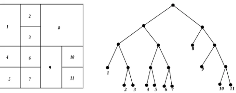
9 10
Figure 11: Example depth-first search for a replacement node
APPENDIX
A.
CAN MAINTENANCE: BACKGROUND
ZONE REASSIGNMENT
The immediate takeover algorithm described in Section 2.3 may result in a single node being assigned multiple zones. Ideally, we would like to retain a one-to-one assignment of nodes to zones, because this prevents the coordinate space from becoming highly fragmented. To achieve this one-to-one node to zone assignment, we use a simple algorithm that aims at maintaining, even in the face of node failures, a dissection of the coordinate space that could have been created solely by nodes joining the system.
At a general step we can think of each existing zone as a leaf of a binary “partition tree.” The internal vertices in the tree represent zones that no longer exist, but were split at some previous time. The children of a tree vertex are the two zones into which it was split. Of course we don’t maintain this partition tree as a data structure, but it is useful conceptually.
By an abuse of notation, we use the same name for a leaf ver-tex, for the zone corresponding to that leaf verver-tex, and for the node responsible for that zone. The partition tree, like any binary parti-tion tree, has the property that in the subtree rooted at any internal vertex there are two leaves that are siblings.
Now suppose a node wants to hand-off a leaf
x
. If the sibling of this leaf is also a leaf (call ity
) the hand-off is easy: simply coalesce leavesx
andy
, making their former parent vertex a leaf, and assign nodey
to that leaf. Thus zonesx
andy
merge into a single zone which is assigned to nodey
. Ifx
’s siblingy
is not a leaf, perform a depth-first search in the subtree of the partition tree rooted aty
until two sibling leaves are found. Call these leavesz
andw
. Combinez
andw
, making their former parent a leaf. Thus zonesz
andw
are merged into a single zone, which is assigned to nodez
, and nodew
takes over zonex
.Figure 11 illustrates this reassignment process. Let us say node 9 fails and by the immediate takeover algorithm node 6 takes over node 9’s place. By the background reassignment process, node 6 discovers sibling nodes 10 and 11. One of these, say 11 takes over the combined zones 10 and 11, and 10 takes over what was 9’s zone.
While the partition tree data structure helps us explain the re-quired transformations, its global nature makes it unsuitable for actual implementation. Instead we must effect the required trans-formations using purely local operations. All an individual node actually has is its coordinate routing table which captures the adja-cency structure among the current zones (the leaves of the deletion tree). However, this adjacency structure is sufficient for emulation of all the operations on the partition tree.
A node
I
performs the equivalent of the above described depth-first search on the partition as follows:Number of dimensions avg(# hops) max(# hops)
2 1.12 3
3 1.09 3
4 1.07 3
Table 6: Background zone reassignment
let
d
kbe the last dimension along which node
I
’s zone washalved (this can be easily detected by merely searching for the highest ordered dimension with the shortest coordinate span).
from its coordinate routing table, node
I
selects a neighbornode
J
that abutsI
along dimensiond
ksuch thatJ
belongsto the zone that forms the other half to
I
’s zone by the last split along dimensiond
k.if the volume of
J
’s zone equalsI
’s volume, thenI
andJ
area pair of sibling leaf nodes whose zones can be combined.
If
J
’s zone is smaller thanI
’s thenI
forwards a depth-firstsearch request to node
J
, which then repeats the same steps.This process repeats until a pair of sibling nodes is found.
We used simulation to measure the number of steps a depth-first search request has to travel before sibling leaf nodes can be found. Table 6 lists the number of hops away from itself that a node would have to search in order to find a node it can hand off an extra zone to. Because of the more or less uniform partitioning of the space (due to our uniform partitioning feature from Section 3.7), a pair of sibling nodes is typically available very close to the request-ing node, i.e., the dissection tree is well balanced.