Notes on Linear Control Systems: Module VII
Stefano Battilotti
Abstract—Controllability and observability. Eigenvalue assign-ment and stabilization via state-feedback. Controllability PBH test. State Observers and detectors. Observability PBH tests. Eigenvalue assignment and stabilization via output-feedback: the separation principle.
I. CONTROLLABILITY
An important problem in control theory is to find an input function which steers the state from an initial value x0 to a final value xf in a given time tf. The characterization of the states which can be reached in time tf from a given statex0 is related to the notion of controllable states.
Definition 1.1: A state xf P Rn is said to be controllable fromx0at timetfif there exists an input functionuandtf ą0
such that
xtfpx0,uq “xf (1)
Therefore, a statexf is controllable from x0 if there exists an input function uwhich steers the solutionxtpx0,uqto the pointxf intf sec. The set of controllable states fromx0:“0 is a vector space.
Proposition1.1: The set of controllable states fromx0“0
is a vector subspace of the state spaceRn.
Therefore, if xa andxb are both controllable from x0“0 thencaxa`cbxb is controllable from x0“0for anyca, cbP
R.
Let xa andxb two controllable states from x0 “0 attf a andtf b. The statecaxa`cbxb for realsca, cb is controllable from x0“0 attf “maxttf a, tf bu.
Now, we want to characterize the set of controllable states in terms of the matricesAandB. To this aim, let us introduce the following time-varying nˆnmatrix
Gptq:“
żJ
0
eAτBBJeAJτ
dτ (2)
This matrix is symmetric and it is known as controllability gramian. Also, define the controllability matrix
R:“`B AB A2B ¨ ¨ ¨ An´1B˘
(3) Proposition1.2:For eacht‰0:SpantGptqu “SpantRu. Moreover, the set of controllable states fromx0“0at timetf
isSpantGptfqu.
Note that, if SpantGptfqu “ Rn, any state xf P Rn is
controllable from x0 :“0 no matter what the final tf is. In this case, by proposition 1.2SpantRu “Rn.
S. Battilotti is with Department of Computer, Control, and Management Engineering “Antonio Ruberti”, Sapienza University of Rome, Via Ariosto 25, Italy.
These notes are directed to MS Degrees in Aeronautical Engineering and Space and Astronautical Engineering. Last update 1/12/2020
Definition1.2: IfSpantRu “Rnthen the system is said to be controllable (or controllable).
Now, we are in a position to characterize any state which is controllable from a givenx0PRn. Since
xtpx0,uq “eAtx0`
żJ
0
eApt´τqBu
τdτ (4) it follows that a statexf is controllable fromx0PRn at time tf if and only ifxf´eAtfx0 is controllable from0 at time
tf.
Proposition 1.3: The set of states controllable at time tf
fromx0 P Rn is the set of statesxf for which xf ´eAtfx0
is controllable at timetf fromx0:“0and it is equal to
tzPRn:z“eAtfx
0`y, yPSpantRuu (5) As a final task, we want to find the input function u for which a state xf is controllable from x0 P Rn at time tf. To this aim, first we find the input function u for which a state xf is controllable is controllable from 0 at time tf. If
xf PSpantGptfqu thenxf is controllable from0 at timetf by proposition 1.2. Therefore, there exists wPRn such that xf“Gptfqw. The input functionudefined as
ut:“BJeA Jpt
f´tqw (6)
is such that
xf “xtfpx0,uq (7)
Indeed,
xtfpx0,uq “
żtf
0
eAptf´τqBu
τdτ
“
żtf
0
eAptf´τqBBJeAJptf´τqwdτ “Gpt
fqw“xf Next, we find the input functionufor whichxfis controllable from x0 P Rn at time tf. If xf ´eAtfx0 P SpantGptfqu then xf ´eAtfx0 is controllable from x0 P Rn at time tf by proposition 1.3. Therefore, if w P Rn is such that xf ´
eAtfx
0“Gptfqw, the input function udefined as
ut:“BJeA Jpt
f´tqw (8)
is such that
xf “xtfpx0,uq (9)
Proposition1.4:IfSpantRu “Rn, any statexf is
control-lable from anyx0within any timetfand an input funtion which
steers the statex0toxfwithintfsec is
ut:“BJeA Jpt
f´tqG´1pt
Exercize1.1:Consider the double integrator
9
x1,t“x2,t
9
x2,t“ut (11)
and calculate the set of controllable states from 0. Determine the input function u(if possible) which steers the state from x0“
`
1 0˘Jtoxf “
`
8 ´6˘Jwithintf“1sec. In this case
A“
ˆ
0 1 0 0
˙
, B“
ˆ
0 1
˙
The controllability matrix is
R:“`B AB˘“
ˆ
0 1 1 0
˙
(12) and SpantRu “ R2, Therefore, the set of controllable states
from 0is R2. Also the set of controllable states from any x0 is R2 (proposition 1.3).
The controllability gramianis
Gptq:“
żJ
0
eAτBBJeAJτ
dτ “ żJ 0 ˆ 1 τ 0 1 ˙ ˆ 0 1 ˙ `
0 1˘
ˆ 1 0 τ 1 ˙ dτ “ żJ 0 ˆ τ 1 ˙ `
τ 1˘dτ “
żJ
0
ˆ
τ2 τ
τ 1 ˙ dτ “ ˆ1 3t 3 1 2t 2 1 2t 2 t ˙ since
eAt“
ˆ
1 t
0 1
˙
(13) Note that SpantRu “ SpantGptfqu “R2 (proposition 1.2)
sinceGptfqis nonsingular for eachtf‰0.
Let us calculate the input function u (if possible) which steers the state from x0 :“
`
1 0˘J to xf “
`
8 ´6˘J (proposition 1.4). Let
w:“G´1ptfqpxf´eAtfx0q
“12 t4 f
ˆ
tf ´12t2f
´12t2 f 1 3t 3 f ˙ r ˆ 8 ´6 ˙ ´ ˆ 1 0 ˙ s “12 t4 f ˆ
7tf`3t2f
´72t2f´2t3f
˙ “ ˆ 120 ´66 ˙ (14) The desired input function is
ut:“BJeA Jp1´tq
w“`1´t 1˘
ˆ
120
´66
˙
“ ´120t`54.Ÿ
Exercize1.2:Consider the model
9
x1,t“ ´x1,t
9
x2,t“x2,t`ut (15)
and calculate the set of controllable states from0. Determine the input functionu(if possible) which steers the state fromx0“
ˆ
2 0
˙
toxf “
`
1 ´6˘Jand, respectively, toxf “
`
4 ´6˘J.
In this case
A“
ˆ
´1 0 0 1
˙
, B“
ˆ
0 1
˙
Thecontrollability matrix is
R:“`B AB˘“
ˆ
0 0 1 1
˙
(16) and SpantRu “ Spant`0 1˘Ju. Therefore, the set of con-trollable states from0is Spant`0 1˘Ju. Since
eAt“
ˆ
e´t 0 0 et
˙
(17) the set of controllable states from anyx0:“
`
x01 x02
˘J
is
tzPRn:z“eAtfx
0`y, yPSpantRuu
“ tzPRn:z“
ˆ
e´tfx
01
c
˙
, cPRu
Therefore the statexf “
`
1 ´6˘Jis controllable fromx0“
`
2 0˘J within tf “ ln2 sec. On the other hand, the state
xf“
`
4 ´6˘J is not controllable fromx0“
`
2 0˘J. Using (17) thecontrollability gramian is
Gptq:“
żJ
0
eAτBBJeAJτ
dτ
“
żJ
0
ˆ
e´τ 0 0 eτ
˙ ˆ
0 1
˙ `
0 1˘
ˆ
e´τ 0 0 eτ
˙ dτ “ żJ 0 ˆ 0 0 0 e2τ
˙
dτ “1
2
ˆ
0 0
0 e2t´1
˙
(18) Note that for eachtf‰0
SpantRu “SpantGptfqu “Span
!ˆ0
1
˙ )
Let us calculate the input function u which steers the state
x0“
`
2 0˘J toxf “
`
1 ´6˘J within tf “ln2 sec. Let
wPR2 be such that xf´eAtfx0“Gptfqw, i.e.
xf´eAln2x0“
ˆ
0
´6
˙
“Gpln2qw“
ˆ 0 0 0 2 ˙ w We obtain
w“ ´3
ˆ
0 1
˙
(19) The desired input function is
ut:“BJeA J
pln2´tqw“ ´3`
0 eln2´t˘ ˆ
0 1
˙
“ ´6e´t.Ÿ
II. OBSERVABILITY
Another important problem in control theory is to recon-struct the intial valuex0 of the state from the observations of the inputs and the outputs. The characterization of the states which can be reconstructed from the inputs and the outputs is related to the notion of unobservable states.
Definition 2.1: Two states xa, xb P Rn are said to be indistinguishable if there existstf ą0such that for any input
functionudefined overr0, tfsand for alltP r0, tfs
Therefore, two states are indistinguishable if they produce as initial conditions the same output under the same input. If the initial state x0 is zero, we have the following definition.
Definition 2.2:A statexPRn is said to be unobservable if there existstf ą 0such that for any input functionudefined
overr0, tfsand for alltP r0, tfs
ytpx,uq “ytp0,uq (21) The set of unobservable states is a vector space.
Proposition 2.1: The set of unobservable states is a vector subspace of the state spaceRn.
Now, we want to characterize the set of unobservable states in terms of the matrices A andC. To this aim, let us introduce the following time-varying nˆnmatrix
GOptq:“
żJ
0
eATτCJCeAτdτ (22) This matrix is symmetric and it is known as observability gramian. At the same time, define the observability matrix
O:“
¨
˚ ˚ ˚ ˝
C CA
.. .
CAn´1
˛
‹ ‹ ‹ ‚
(23)
Proposition 2.2:For eacht ‰0:KertGOptqu “KertOu.
Moreover, the set of unobservable states isKertGOptfqu. Note that, if KertGOptfqu “ t0u, the only unobservable state is x“0 whatever the observation interval r0, tfs is. In this case, by proposition 2.2KertOu “ t0u.
Definition 2.3: IfKertOu “ t0uthen the system is said to be observable.
Now, we are in a position to characterize the statesxawhich are indistinguishable from a givenxb. Since
ytpxa,uq “ytpxb,uq, @tP r0, tfs
ôytpxa´xb,uq “ytp0,uq, @tP r0, tfs (24) it follows that xa is indistinguishable from a given xb if and only if xa´xb is unobservable.
Proposition 2.3: The set of statesxa is indistinguishable
from a given xb is the set of statesxa for whichxa ´xb is
unobservable and it is equal to
tzPRn:z“xb`y, yPKertOuu (25) Relying on the previous characterizations, we study how to reconstruct the initial states x0 (and, therefore, the entire solutionxtpx0,uq) from the observation of the inputs and the outputs over a time interval r0, tfs. The reconstruction ofx0 can be related to the observability gramianGO. Indeed, from the observation of the inputuand the ensuing outputytpx0,uq over the time intervalr0, tfswe obtain the zero input-to-output response
ytpunf orcedqpx0q “ytpx0,uq ´
żJ
0
eApt´τqBu
τdτ
If the system is observable we claim that x0 can be recon-structed from
żtf
0
eAJθCJypunf orcedq
θ px0qdθ
Indeed,
żtf
0
eAJθCJypunf orcedq
θ px0qdθ
“
żtf
0
eAJθCTCeAθx0dθ“GOptfqx0
and therefore
x0“G´O1ptfq
żtf
0
eAJθCTypθunf orcedqpx0qdθ
Proposition 2.4: IfKertOu “ t0u, the only unobservable state is0and the initial statex0can be reconstructed from the
observation of the input uand the ensuing output ytpx0,uq
over the time intervalr0, tfs,tfą0, as
x0“G´O1ptfq ˆ
ˆ
żtf
0
eAJθCJ´y
θpx0,uq ´
żtf
0
eApθ´τqBu
τdτ
¯
dθ
Exercize2.1:Consider the double integrator
9
x1,t“x2,t
9
x2,t“ut
yt“x1,t
and calculate the set of unobservable states. Reconstruct the initial value of the statex0from the unforced output response 1`tover the time intervalr0, tfswithtf “1sec.
In this case
A“
ˆ
0 1 0 0
˙
, B“
ˆ
0 1
˙
, C “`1 0˘
Theobservability matrix is
O:“
ˆ
C CA
˙
“
ˆ
1 0 0 1
˙
(26) andKertOu “ t0u. Therefore, the set of unobservable states ist0u. Also the set of indistinguishable states from anyxa is
txau.
Theobservability gramian GOptq:“
żJ
0
eATτCJCeAτdτ
“
żJ
0
ˆ
1 0
τ 1
˙ ˆ
1 0
˙ `
1 0˘
ˆ
1 τ
0 1
˙
dτ
“
żJ
0
ˆ
1
τ
˙ `
1 τ˘dτ “
żJ
0
ˆ
1 τ τ τ2
˙
dτ “
ˆ
t 1 2t
2 1 2t
2 1 3t
3
˙
since
eAt“
ˆ
1 t
0 1
˙
(27) Note that KertOu “ KertGOptfqu “ t0u since GOptfq is nonsingular for eachtf‰0. Next, we see how to reconstruct
x0 from the unforced output response 1`t over the time intervalr0, tfswithtf “1 sec. Then
G´O1ptfqeA
Tt
CJ“ 12 t4
f
ˆ 1 3t
3 f ´
1 2t
2 f
´12t2f tf
˙ ˆ
1
t
˙
“ 12 t4
f
ˆ1 3t
3 f´
1 2t
2 ft
´12t2f`tft
˙
“12
ˆ1
3´ 1 2t
´12`t
˙
The initial state x0 is reconstructed from the zero input-to-output response1`t as
x0“G´O1ptfq
żtf
0
eAJθCJypunf orcedq
θ px0qdθ
“12
ż1
0
ˆ1 3 ´
1 2θ
´12`θ
˙
p1`θqdθ
“12
ż1
0
ˆ1 3 ´
1 2θ
´12`θ
˙
p1`θqdθ“
ˆ
1 1
˙
.Ÿ
Exercize2.2:Consider the model
9
x1,t“ ´x1,t
9
x2,t“x2,t`ut
yt“x2,t (29)
and calculate the set of indistinguishable states from x “
`
1 1˘J.
In this case
A“
ˆ
´1 0 0 1
˙
, B“
ˆ
0 1
˙
, C“`0 1˘
The observability matrix is
O:“
ˆ
C CA
˙
“
ˆ
0 1 0 1
˙
(30) and KertOu “Spant`1 0˘Ju, Therefore, the set of unob-servable states is
KertOu “Span
!ˆ1
0
˙ )
(propositions 2.2). The set of indistinguishable states fromx“
`
1 1˘J is
tzPRn:z“x`y, yPKertOuu “ tzPRn :z“
ˆ
c
1
˙
, cPRu
Therefore, all the initial states `c 1˘J, c P R, cannot
be reconstructed from the observation of the input u and the ensuing output ypt, x0,uq over any time interval r0, tfs,
tf ą0. Ÿ
III. EIGENVALUES ASSIGNMENT AND STABILIZATION
We have seen that for controllable systems it is possible to drive the state from any initial state x0 to0 within any given timetf with an input function
ut:“ ´BJeA Jpt
f´tqG´1pt
fqeAtfx0
whereGptfqis the controllability gramian. We have also seen that this control input lacks in robustness. In this section, we want to study the problem of steering all the states from any initial state x0 to 0 within an infinite time interval(i.e. tf “
`8) with a given convergence rate. This can be formulated as a problem of “assigning” the eigenvalues of the matrix A
in such a way that the natural modes are all convergent with the given convergence rates.
A. Eigenvalues assignment via state feedback
Consider the class of control laws
ut“Fxt`vt (31) with matrix Fp1ˆnq andv is the new control input. These control laws are commonly referred to asstatic state feedback
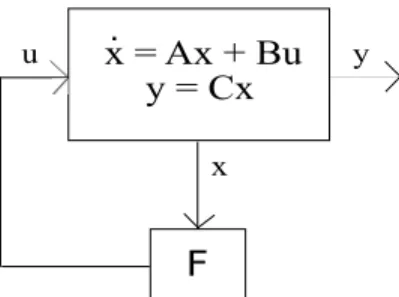
laws, in the sense that the state information is used to imple-ment the control law and the relation betweenxandvon one side anduon the other is instantaneous, i.e. no dynamics. The systemx9t“Axt`But, subject to the control input (31), is represented by the new equations
9
xt“ pA`BFqxt`Bvt (32) In other words, the matrixAhas been changed intoA`BF
(see Figure 1). If we are able to find a matrix F in such a way that the eigenvalues of A`BF are equal to a given set
tλ˚
1, . . . , λ˚nu ĂC, then the natural modes are all convergent with rate convergence corresponding to the given negative real parts. On the other hand, this guarantees also asymptotic stability of (32). This problem can be formulated as follows. LetσpNqdenote the spectrumof a square matrixN, i.e. the set of its eigenvalues.
Definition 3.1: (Spectrum assignment by state feedback). Given numberstλ˚
1, . . . , λ˚nu,λ˚i P C´ for all i “ 1, . . . , n,
either real or complex conjugate, find a matrixFp1ˆnqsuch thatσpA`BFq “ tλ˚
1, . . . , λ˚nu.
A necessary and sufficient condition for the existence ofF
is the following.
Proposition 3.1: The Spectrum assignment by state feed-back problem is solvable if and only if the system is control-lable, i.e. the controllability matrixRis nonsingular. In particu-lar, ifR is nonsingular then for given numberstλ˚
1, . . . , λ˚nu,
λ˚
i P C´ for all i “ 1, . . . , n, the Spectrum assignment
problem is solvable with
F “ ´γp˚pAq (33) whereγis the last row ofR´1andp˚pλq:“śn
j“1pλ´λ˚jq.
1) Controllability as a necessary condition for the solvabil-ity of the Spectrum assignment problem: We want to show that a necessary condition for the solvability of the Spectrum assignment by state feedback problem is the controllability of the system. To this aim, we will assume to have a matrix F
which solves the Spectrum assignment problem. If the system is not controlable, we will come to a contradiction. Indeed, if the system not controlable,Ris not nonsingular and say
nąr:“rankRtRu
Letv1, . . . , vrPRn be a base of SpantRu(we may assume
that vi:“Ai´1B,i“1, . . . , r, i.e. the firstrcolumns of R) and define
T :“`v1 ¨ ¨ ¨ vr w1 ¨ ¨ ¨ wn´r
˘´1
(34) where w1, . . . , wn´r P Rn are such that v1, . . . , vr, w1, . . . , wn´r altogether are a basis of Rn,
i.e. the matrix
`
v1 ¨ ¨ ¨ vr w1 ¨ ¨ ¨ wn´r
x = Ax + Bu
.F
ux
y
y = Cx
Figure 1. Control scheme for eigenvalue assignment by state feedback.
is nonsingular. If we transform the state as z“T x this will induce a transformation on the matrices A, B, F as follows
˜
A“T AT´1, ; ˜B
“T B, F˜ “F T. (35) It can be seen that there exist matrices A˜11prˆrq,A˜12prˆ
pn´rqq,A˜22ppn´rq ˆ pn´rqqandB˜1prˆ1qsuch that
˜
A“T AT´1
“
ˆ˜
A11 A˜12 0 A˜22
˙
, B˜“T B“
ˆ˜
B1 0
˙
(36) (this follows from ASpantRu Ă SpantRu and B P
SpantRu).
Note that for allλPCn
detpλI´ pA˜`B˜Fqq “˜ detpλI´TpA`BFqT´1
q “detpTpλI´ pA`BFqqT´1
q “detTdetpλI´ pA`BFqqdetT´1
and, therefore, the roots ofdetpλI´ pA˜`B˜F˜qqanddetpλI´ pA`BFqqare the same, i.e.
σpA˜`B˜F˜q “σpA`BFq (37)
From (36) and writing F˜ :“ `F˜1 F˜2
˘
for some matrices ˜
F1p1ˆrq andF˜2p1ˆ pn´rqq, then
σpA`BFq “σpA˜`B˜F˜q
“σ
ˆ˜
A11`B˜1F˜1 A˜12`B˜1F˜2
0 A˜22
˙
“σpA˜11`B˜1F˜1q YσpA˜22q
Moreover, σpA˜22q Ă σpAq since σpAq “˜ σpAq. It follows that the eigenvalues of Awhich correspond toσpA˜22qcannot be changed into any given subset of tλ˚
1, . . . , λ˚nu and this contradicts the existence of F which solves the Spectrum assignment problem.
2) Controllability as a sufficient condition for the solvability of the Spectrum assignment problem: Ackermann formula for spectrum assignment: Next, we want to show that a sufficient condition for the solvability of the Spectrum assignment by state feedback problem is the controllability of the system. This is the constructive part of our result and gives a matrix
F, defined in (33), which assigns the given spectrum to the matrix A(i.e. solves the Spectrum assignment problem).
Assume that the system is controllable, i.e.Ris nonsingular. Letγbe the last row ofR´1and define the realsa˚
0, . . . , a˚n´1 in such a way that
p˚pλq: “
n
ź
j“1
pλ´λ˚
jq :“a˚
0`a˚1λ` ¨ ¨ ¨ `a˚n´1λ n´1
`λn (38) Note that the roots of p˚pλq are exactly the given tλ˚
1, . . . , λ˚nu.
We will outline the procedure for obtaining the matrixF in suitable new coordinates F˜ (for which the matricesA andB
have ad hoc expressions) and then back to F in the original coordinates. Define
T :“
¨
˚ ˚ ˚ ˝
γ γA
.. .
γAn´1
˛
‹ ‹ ‹ ‚
It can be shown thatT is nonsingular (this follows from the invertibility of R). It can be also seen that
˜
A“T AT´1
“
¨
˚ ˚ ˚ ˚ ˚ ˝
0 1 0 ¨ ¨ ¨ 0 0 0 0 1 ¨ ¨ ¨ 0 0
..
. ... ... ¨ ¨ ¨ ... ... 0 0 0 ¨ ¨ ¨ 0 1
´a0 ´a1 ´a2 ¨ ¨ ¨ ´an´2 ´an´1
˛
‹ ‹ ‹ ‹ ‹ ‚
(39)
and
˜
B“T B“
¨
˚ ˚ ˚ ˚ ˚ ˝
0 0 .. . 0 1
˛
‹ ‹ ‹ ‹ ‹ ‚
(40)
where a0, . . . , an´1 are the coefficients of the characteristic polynomialppλqof A:
ppλq “a0`a1λ` ¨ ¨ ¨ `an´1λn´1`λn (41) Define
˜
F
:“`a0´a˚0 a1´a˚1 ¨ ¨ ¨ an´2´a˚n´2 an´1´a˚n´1
then
˜
A`B˜F˜ “
¨
˚ ˚ ˚ ˚ ˚ ˝
0 1 0 ¨ ¨ ¨ 0 0 0 0 1 ¨ ¨ ¨ 0 0
..
. ... ... ¨ ¨ ¨ ... ... 0 0 0 ¨ ¨ ¨ 0 1
´a˚
0 ´a˚1 ´a˚2 ¨ ¨ ¨ ´a˚n´2 ´a˚n´1
˛
‹ ‹ ‹ ‹ ‹ ‚
(42)
and
detpλI´ pA˜`B˜F˜qq “a˚
0`a˚1λ` ¨ ¨ ¨ `a˚n´1λ n´1
`λn“p˚pλq (43)
Therefore, tλ˚
1, . . . , λ˚nu are the eigenvalues of A˜ ` B˜F˜. Getting back in original coordinates
F :“F T˜ (44) ButσpA˜`B˜Fq “˜ σpA`BFq. Indeed,
detpλI´ pA˜`B˜Fqq “˜ detpλI´ pT AT´1
`T BF T T˜ ´1
qq “detpTpλI´ pA`BFqqT´1q
“detTdetpλI´ pA`BFqqdetT´1
We conclude that the Spectrum assignment problem by state feedback is solved by F in (44). Moreover, it is easy to see, after some manipulations, that
F “ ´γp˚pAq (45) whereγ is the last row ofR´1 and
p˚pAq “a
0I`a1A` ¨ ¨ ¨ `an´1An´1`An. (46) The above formula (45) forF is known as Ackermann formula for spectrum assignment.
B. Stabilization via state feedback
If the system is not controllable there is a subset of the eigenvalues ofA`BF that are invariant under any choice of
F (invariant spectrum). This subset is exactly the spectrum of the matrixA˜22(see (36)) which is a subset of the spectrum of
A. The matrixA˜22 can be calculated fromT AT´1 whereT is defined as in (34). Even if the system is not controlable, it is possible to find a F such thatσpA`BFq “ tλ˚
1, . . . , λ˚nu as long as the invariant spectrum ofA`BF is a subset of the given settλ˚
1, . . . , λ˚nu. Denote byFR this invariant spectrum of A`BF.
Proposition3.2:Given numberstλ˚
1, . . . , λ˚nu,λ˚i PC´for
alli“1, . . . , n, either real or complex conjugate, there exists a matrixFp1ˆnqsuch thatσpA`BFq “ tλ˚
1, . . . , λ˚nuif and
only ifFRĂ tλ˚1, . . . , λ˚nu.
1) Design of stabilizing state feedback controllers: We show how to design F when FR Ă L “ tλ˚1, . . . , λ˚nu. Let
r:“rankRtRu. Under the coordinate transformationz“T x, where T is defined as in (34), the matrices A and B are trasformed into
˜
A“
ˆ˜
A11 A˜12 0 A˜22
˙
, B˜ “
ˆ˜
B1 0
˙
(47)
withA˜11prˆrq,A˜12prˆ pn´rqq,A˜22ppn´rq ˆ pn´rqqand ˜
B1prˆ1q. We want to show that
rankR`B˜1 A˜11B˜1 ¨ ¨ ¨ A˜r11´1B˜1
˘
“r (48) This means that the Eigenvalues assignment problem is solv-able with matrices A˜11 and B˜1. As a matter of fact, since
T AjT´1“ pT AT´1
qj “A˜j for all integerj, we have
r“rankRtRu “rankRt`B AB ¨ ¨ ¨ An´1B˘
u “rankRtT`B AB ¨ ¨ ¨ An´1B˘
u “rankRt`T B T AT´1T B
¨ ¨ ¨ T An´1T´1T B˘
u “rankRt`B˜ A˜B˜ ¨ ¨ ¨ A˜n´1B˜˘
u “rankR
!ˆB˜
1 0
˜
A11B˜1 0 ¨ ¨ ¨
˜
Ar´1 11 B˜1
0
˙)
“rankRt`B˜1 A˜11B˜1 ¨ ¨ ¨ A˜r11´1B˜1
˘
u (49) i.e. (48). Define
˜
F :“`F˜1 0
˘
(50) withF˜1p1ˆrqsuch that
σpA˜11`F˜1B˜1q “LzFR
(F˜1exists by virtue of (48) and proposition 3.1) and
F :“F T˜ (51) Note that for allλPCn
detpλI´ pA˜`B˜F˜qq “detpλI´TpA`BFqT´1
q “detpTpλI´ pA`BFqqT´1
q “detTdetpλI´ pA`BFqqdetT´1
and, therefore, the roots ofdetpλI´ pA˜`B˜F˜qqanddetpλI´ pA`BFqqare the same, i.e.
σpA˜`B˜F˜q “σpA`BFq (52) Moreover,
σpA`BFq “σpA˜`B˜F˜q “σpA˜11`B˜1F˜1q YσpA˜22q
“σpA˜11`B˜1F˜1q YFR“L
The construction of the matrix F can be summed up as follows:
Step procedure for the design of stabilizing state-feedback controllers
(i) Let r :“ rankRtRu. Find w1, . . . , wn´r such that
B, AB,¨ ¨ ¨, Ar´1B, w
1, . . . , wn´ris a basis ofRnand define T as
T :“`B AB ¨ ¨ ¨ Ar´1B w
1 ¨ ¨ ¨ wn´r
˘´1 (53)
(ii)Find the matricesA˜11prˆrq,A˜12prˆ pn´rqq,A˜22ppn´
rq ˆ pn´rqqandB˜1prˆ1qfor which
˜
A“T AT´1
“
ˆ˜
A11 A˜12 0 A˜22
˙
, B˜ “T B“
ˆ˜
B1 0
˙
(54)
(iii) Find F˜1p1ˆrq such that σpA˜11`F˜1B˜1q “ LzFR. In particular,
˜
where p˚
spλq :“ α˚0 `α˚1λ` ¨ ¨ ¨ `α˚r´1λr´1 `λr is the polynomial which has the roots in LzFR and
p˚
spA˜11q:“α˚0I`α˚1A˜11` ¨ ¨ ¨ `α˚r´1A˜ r´1 11 `A˜
r 11 (56) andγs is the last row of the inverse of
Rs:“
`˜
B1 A˜1B˜1 ¨ ¨ ¨ A˜r1´1B˜1
˘
(57)
(iv) Define
˜
F :“`F˜1 0
˘
(58) and, finally, set
F :“F T˜ (59) Exercize3.1:Given
A“
ˆ
´1 0 1 ´2
˙
, B“
ˆ
1
β
˙
, β PR (60)
find, if possible,F such thatσpA`BFq “ t´2,´2u.
The controllability matrix R is
R“`B AB˘“
ˆ
1 ´1
β 1´2β
˙
Therefore, the system is controllable if and only if β‰1.
Caseβ “1. The system is not controllable. We use proposition 3.2. In this case we have to check if the invariant spectrum of
A is a subset oft´2,´2u. Note that
r:“rankRtRu “rankRt`B AB˘u
“rankR
!ˆ1 ´1
1 ´1
˙ )
“1 (61)
For calculating the invariant spectrum of A, we change the coordinates as follows. A basis ofSpantRuis
v1:“
ˆ
1 1
˙
(we can take the first column of Rsincer“1). Define
T “`v1 w1
˘
“
ˆ
1 1 1 ´1
˙´1
“ 1
2
ˆ
1 1 1 ´1
˙
In the new coordinatesz“T x
˜
A“T AT´1
“
ˆ
´1 1 0 ´2
˙
, B˜“B“
ˆ
1 0
˙
(62) Sincer“1,A˜11“ ´1,A˜12“1,A˜22“ ´2andB˜1“1and we conclude that the invariant spectrum is FR :“σpA˜22q “
t´2u. Since FR :“ t´2u ĂL :“ t´2,´2u, by proposition 3.2 there exists F such that σpA`BFq “ t´2,´2u. Let construct this matrix F. We have
˜
F :“`F˜1 0
˘
(63) whereF˜1 is such thatσpA˜11`B˜1F˜1q “LzFR“ t´2u. Such
˜
F1 exists sinceA˜11 and B˜1 represent a controllable system, indeed
rankRtB˜1u “1“r (64) On the hand,σpA˜11`B˜1F˜1q “ t´2uif and only ifF˜1“ ´1. Finally, define
F :“F T˜ “`´1 0˘T “ ´1
2
`
1 1˘ (65)
We can check that
σpA`BFq “σ
´ˆ´1 0
1 ´2
˙
´1
2
ˆ
1 1
˙ `
1 1˘
¯
“σ
ˆ
´32 ´12
1
2 ´
5 2
˙
“ t´2,´2u (66)
Caseβ ‰1. The system is controllable. In this case we use proposition 3.1. The spectrum to be assigned ist´2,´2uand, therefore,
p˚pλq:“ pλ`2q2
The matrixF which solves the Spectrum assignment problem by state feedback withL:“ t´2,´2uis
F “ ´γp˚pAq (67)
whereγ is the last row ofR´1. Since
R“`B AB˘“
ˆ
1 ´1
β 1´2β
˙
then
R´1
“ 1
1´β
ˆ
1´2β 1
´β 1
˙
and
γ:“ 1
1´β
`
´β 1˘ Moreover
p˚pAq:“ pA`2Iq2
“A2`4A`4I
“
ˆ
´1 0 1 ´2
˙2
`4
ˆ
´1 0 1 ´2
˙
`4
ˆ
1 0 0 1
˙
“
ˆ
1 0 1 0
˙
Finally,
F “ ´γp˚pAq “ ´ 1
1´β
`
´β 1˘
ˆ
1 0 1 0
˙
“`´1 0˘(68) We can check that
σpA`BFq “σ´
ˆ
´1 0 1 ´2
˙
`
ˆ
1
β
˙ `
´1 0˘¯
“σ
ˆ
´2 0 1´β ´2
˙
“ t´2,´2u.Ÿ (69)
C. The controllability PBH test
The invariant spectrum FR of A`BF can be determined without a coordinate transformation by calling upon the so-called controllability PBH test (PBH stands for the authors Popov, Belevitch, Hautus).
Proposition3.3:(Controllability PBH test). A necessary and sufficient condition for reachability, i.e.Rnonsingular, is
rankRt`λI´A B˘u “n for eachλPσpAq. Moreover,
rankRt`λI´A B˘u
#ăn ñλPF
R
“n ñλRFR
(70)
Proposition3.4:(Controllability PBH test). A necessary and sufficient condition for reachability, i.e.Rnonsingular, is that
for eachλPCn.
Exercize 3.2:We want to revisit the results of example 3.1 through the PBH controllability test.
Caseβ“1. The system is not controllable. It is easily seen that σpAq “ t´1,´2u. By proposition 3.3
λ“ ´2ñrankRt`λI´A B˘u
“rankR
!ˆ´1 0 1
´1 0 1
˙ )
“1ăn“2ñ t´2u PFR
and
λ“ ´1ñrankRt`λI´A B˘u
“rankR
!ˆ 0 0 1
´1 1 1
˙)
“2“nñ t´1u RFR
Therefore, there existsF such that σpA`BFq “ t´2,´2u.
Caseβ ‰1. The system is controllable andFR is empty. By proposition 3.3
λ“ ´2ñrankRt`λI´A B˘u
“rankR
!ˆ´1 0 1
´1 0 β
˙)
“2“nñ t´2u RFR
and
λ“ ´1ñrankRt`λI´A B˘u
“rankR
!ˆ 0 0 1
´1 1 β
˙)
“2“nñ t´1u RFR.Ÿ
D. Design of asymptotic observers
We have seen that for observable systems it is possible to reconstruct the initial state x0, and therefore, the state
xtpx0,uq, through the observations of the unforced output response yptunf orcedqpx0qover a time intervalr0, tfsas
x0“G´O1ptfq
żtf
0
eAJθCJyptunf orcedqpx0qdθ
where GOp¨q is the observability gramian. In this section, we want to study the problem of reconstructing or estimating the state xtpx0,uq through observations of y and uover an
infinite time interval(i.e. T “ `8) with a given convergence rate. This can be formulated as a problem of “assigning” the convergence rate of the error between the state and its reconstruction. Consider the class of “state estimators”
9
p
xt“Apxt`But`Kpyt´Cxptq. (71)
If e:“x´pxis theestimation error, then the error dynamics is described by the equations
9
et“x9t´px9t
“Axp`But`Kpyt´Cpxtq ´Axt´But
“ pA´KCqet, (72) with matrixKpnˆ1q. If we are able to find a matrixKin such a way that the eigenvalues ofA´KC are equal to a given set
tλ˚
1, . . . , λ˚nuwith negative real part, then the natural modes of (72) are all convergent with rate convergence corresponding to the given negative real parts and the state is reconstructed from the output with the assigned rate. The system (71) is known as
asymptotic state observerand dynamically and asymptotically reconstructs the state xtwithpxt.
Our problem can be formulated as follows.
Definition 3.2:(Asymptotic state observation). Given num-bers tλ˚
1, . . . , λ˚nu, λ˚i P C´ for all i “ 1, . . . , n, either
real or complex conjugate, find a matrixKpnˆ1qsuch that σpA´KCq “ tλ˚
1, . . . , λ˚nu. Note that
σpA´KCq “σppA´KCqJq “σpAJ
´CJKJ
q (73) If we establish the following equivalences
AØAJ B ØCJ
F Ø ´KJ (74) we find out that it is possible to assign the eigenvalues of
A´KC with some matrixKif and only it is possible to assign the eigenvalues of A`BF with some matrix F. Therefore, a necessary and sufficient condition for the existence of K
comes directly from proposition 3.5.
Proposition3.5:The Asymptotic state observation problem is solvable if and only if the system is observable, i.e. the observability matrix O is nonsingular. In particular, if O is nonsingular then for any given numberstλ˚
1, . . . , λ˚nu,λ˚i PC´
for alli“1, . . . , n, the Asymptotic state observation problem is solvable with
K“p˚pAqδ (75) whereδis the last column ofO´1andp˚pλq:“śn
j“1pλ´λ˚jq.
1) Observability as a sufficient condition for the solvability of the asymptotic state observation problem: dual Ackermann formula: Since the assignment of the eigenvalues ofA´KC
with some matrix K is equivalent to the assignment of the eigenvalues of A ` BF with some matrix F under the equivalences (74), by proposition 3.1 the Asymptotic state observation problem is solvable if and only the controllability matrix defined withAØAJ andB ØCJ, i.e. the matrix
R:“`CJ AJCJ ¨ ¨ ¨ pAJqn´1CJ˘
(76) is nonsingular. Since for alljPN
pAJ
qj “ pAjqJ (77) and
R:“`CJ AJCJ ¨ ¨ ¨ pAJqn´1CJ˘
“
¨
˚ ˚ ˚ ˝
C CA
.. .
CAn´1
˛
‹ ‹ ‹ ‚
J
“OT (78)
it follows that the Asymptotic state observation problem is solvable if and only the observability matrix is nonsingular.
Moreover, by proposition 3.1 ifO is nonsingular and under the equivalences (74), for any given numbers tλ˚
1, . . . , λ˚nu,
λ˚
i PC´for alli“1, . . . , n, the Asymptotic state observation problem is solvable with
´KJ:
“F “ ´γp˚pAT
whereγ denotes the last row of
R´1
“`CJ AJCJ ¨ ¨ ¨ pAJqn´1CJ˘´1 (80) We have by changing signs and transposing (79)
K“ pp˚pAT
qqJγT (81) On account of (77)
pp˚pATqqJ“ pa0I`a1AJ`a2pAJq2`. . .
`an´1pAJqn´1` pAJqnqJ
pp˚pAT
qqJ“ pa0I`a1AJ`a2pA2qJ`. . .
`an´1pAn´1qJ` pAnqJqJ
“a0I`a1A`a2A2` ¨ ¨ ¨ `an´1An´1`An “p˚pAq Also, note that since transpose and inverse commute
´`
CJ AJCJ ¨ ¨ ¨ pAJqn´1CJ˘´1¯J
“
˜˜ ¨
˚ ˚ ˚ ˝
C CA
.. .
CAn´1
˛
‹ ‹ ‹ ‚
T
¸´1¸J “
˜˜ ¨
˚ ˚ ˚ ˝
C CA
.. .
CAn´1
˛
‹ ‹ ‹ ‚
T
¸J¸´1
“O´1
and sinceγ is the last row of the matrix inside the transpose on the left of the first equality, it follows that δ:“γJis the
last column of O´1. This gives (75) back.
2) Observability as a necessary condition for the solvability of the asymptotic state observation problem: Let’s see that observability is a necessary condition for the solvability of the Asymptotic state observation problem. If the system is not observable, under the equivalences (74) there exist nonsingular
Tpnˆnqand matricesA˜J
11psˆsq,A˜J12psˆ pn´sqq,A˜J22ppn´
sq ˆ pn´sqqandC˜J
1psˆ1q, with
s:“rankRt`CJ AJCJ ¨ ¨ ¨ pAJqn´1CJ˘
u “rankRtOJu “rank
RtOu (82)
such that
T AJT´1
“
ˆ˜
AT 11 A˜J12 0 A˜J
22
˙
, T CJ “
ˆ˜
CJ
1 0
˙
(83) Indeed,T is defined as follows. Letv1, . . . , vsPRnbe a base
of
Spant`CJ AJCJ ¨ ¨ ¨ pAJqn´1CJ˘
u “SpantOJ u
(we may assumevi:“ pAJqi´1CJ) and
T :“`v1 ¨ ¨ ¨ vs w1 ¨ ¨ ¨ wn´s
˘´1
(84) wherew1, . . . , wn´sPRn are chosen independent each other
and fromv1,¨ ¨ ¨, vs, i.e.v1,¨ ¨ ¨, vs, w1,¨ ¨ ¨, wn´sare a basis of Rn. Taking transposes in (83), we conclude that there exist
matricesA˜11psˆsq,A˜12ppn´sq ˆsq,A˜22ppn´sq ˆ pn´sqq andC˜1p1ˆsqsuch that
SAS´1
“
ˆ˜
A11 0 ˜
A12 A˜22
˙
, CS´1
“`C˜1 0
˘
(85)
whereS :“ pTJq´1“ pT´1
qJ. Note that, since inverse and transpose commute so that
S:“ pTJ q´1“
¨
˚ ˚ ˚ ˚ ˚ ˚ ˚ ˚ ˚ ˚ ˝
C CA
.. .
CAn´s´1
wJ
1 .. .
wJ
s
˛
‹ ‹ ‹ ‹ ‹ ‹ ‹ ‹ ‹ ‹ ‚
(86)
E. Design of state detectors
It is clear from (85) that if the system is not observable there is a non-empty subset of the eigenvalues of A´KC
that is invariant under any choice of K (invariant spectrum). In this case, the system (71) is known as state detector and dynamically and asymptotically reconstructs the statextwith
p
xtbut not with guaranteed rate (since some of the eigenvalues ofA´KCare not assignable). The invariant subset under any choice of K is exactly the spectrum of the matrixA˜22 (see 85) which is a subset of the spectrum ofA. Indeed, with the coordinate transformation z “ Sx the matrices A´KC is transformed intoA˜´K˜C˜ with
˜
A“SAS´1
“
ˆ˜
A11 0 ˜
A12 A˜22
˙
, C˜ “CS´1
“`C˜1 0
˘
(87) and
˜
K“SK (88)
Note that for allλPCn
detpλI´ pA˜´K˜Cqq “˜ detpλI´SpA´KCqS´1q “detpSpλI´ pA´KCqqS´1
q “detSdetpλI´ pA´KCqqdetS´1
and, therefore, the roots of detpλI ´ pA˜ ´K˜Cqq˜ and of detpλI´ pA´KCqqare the same, i.e.
σpA˜´K˜Cq “˜ σpA´KCq (89) Assuming that
˜
K:“
ˆ˜
K1 ˜
K2
˙
for some matricesK˜1psˆ1qandK˜2ppn´sq ˆ1q, then
σpA´KCq “σpA˜´K˜Cq “˜ σ
ˆ˜
A11´K˜1C˜1 0 ˜
A12´K˜2C˜1 A˜22
˙
“σpA˜11´K˜1C˜1q YσpA˜22q (90) Moreover,σpA˜22q ĂσpAqsinceσpAq “˜ σpAq. It follows that the eigenvalues ofAwhich correspond toσpA˜22qare invariant under any choice ofK. The matrixA˜22can be calculated from
SAS´1 whereS is defined as in (86).
Even if the system is not observable, it is possible to find a K such that σpA´KCq “ tλ˚
1, . . . , λ˚nu as long as the invariant spectrum of A´KC is a subset of the given set
tλ˚
1, . . . , λ˚nu. Denote by FO this invariant spectrum of A´
Proposition3.6:Given numberstλ˚
1, . . . , λ˚nu,λ˚i PC´for
alli“1, . . . , n, either real or complex conjugate, there exists a matrixKpnˆ1qsuch thatσpA´KCq “ tλ˚
1, . . . , λ˚nuif and
only ifFOĂ tλ˚1, . . . , λ˚nu.
Let’s see how to construct K if FO ĂL:“ tλ˚1, . . . , λ˚nu. Assume that FO ĂL:“ tλ˚1, . . . , λ˚nu. Let s:“rankRtOu.
Under the coordinate transformation z “T x the matrices A
andC are transformed into ˜
A“
ˆ˜
A11 0 ˜
A12 A˜22
˙
, C˜ “`C˜1 0
˘
(91) withA˜11psˆsq,A˜12ppn´sq ˆsq,A˜22ppn´sq ˆ pn´sqqand
˜
C1p1ˆsq. We want to show that
rankR ! ¨ ˚ ˚ ˚ ˝ ˜ C1 ˜
C1A˜11 .. . ˜
C11A˜s11´1
˛ ‹ ‹ ‹ ‚ )
“s (92)
This means that the Asymptotic state observation problem is solvable with matrices C˜1 and A˜11 (proposition 3.5). As a matter of fact, since SAjS´1 “ pSAS´1
qj “ A˜j for all integer j, we have
s“rankRtOu
“rankR
! ¨ ˚ ˚ ˝ C CA ¨ ¨ ¨ CAn´1
˛
‹ ‹ ‚
)
“rankR
! ¨ ˚ ˚ ˝ C CA ¨ ¨ ¨ CAn´1
˛
‹ ‹ ‚
T´1)
“rankR!
¨
˚ ˚ ˚ ˝
CT´1
CT´1T AT´1
¨ ¨ ¨
CT´1T An´1T´1)
˛
‹ ‹ ‹ ‚
“rankR!
¨ ˚ ˚ ˝ ˜ C ˜
CA˜ ¨ ¨ ¨
˜
CA˜n´1
˛
‹ ‹ ‚
)
“rankR!
¨ ˚ ˚ ˚ ˚ ˚ ˚ ˚ ˚ ˚ ˚ ˚ ˝ ˜ C1 ˜
C1A˜11 .. . ˜
C1A˜s11´1 ˜
C1A˜s11 .. . ˜
C1A˜n11´1 0 0 .. . 0 0 .. . 0 ˛ ‹ ‹ ‹ ‹ ‹ ‹ ‹ ‹ ‹ ‹ ‹ ‚ )
“rankR!
¨ ˚ ˚ ˚ ˝ ˜ C1 ˜
C1A˜11 .. . ˜
C1A˜s11´1
˛ ‹ ‹ ‹ ‚ ) (93) Define ˜
K:“
ˆ˜
K1 0
˙
(94) withK˜1psˆ1qsuch that
σpA˜11´C˜1K˜1q “LzFO
(K˜1 exists by virtue of (92) and proposition 3.5) and
K:“S´1K˜ (95) Note that for allλPCn
detpλI´ pA˜´K˜Cqq “˜ detpλI´SpA´KCqS´1q “detpSpλI´ pA´KCqqS´1
q “detSdetpλI´ pA´KCqqdetS´1
and, therefore, the roots of detpλI ´ pA˜ ´K˜Cqq˜ and of detpλI´ pA´KCqqare the same, i.e.
σpA˜´K˜Cq “˜ σpA´KCq (96) Assuming that
˜
K:“
ˆ˜
K1 ˜
K2
˙
for some matricesK˜1psˆ1qandK˜2ppn´sq ˆ1q, then
σpA´KCq “σpA˜´K˜Cq “˜ σpA˜11`C˜1K˜1q YσpA˜22q
“σpA˜11`C˜1K˜1q YFO“L
The construction of the matrix K can be summed up as follows:
Step procedure for the design of state detectors:
(i) Let s :“ rankRtOu. Find w1, . . . , ws P Rn such that CJ,pCAqJ,¨ ¨ ¨ ,pCAn´s´1
qJ, w1,¨ ¨ ¨ , wsare a basis ofRn
and define S as
S“ ¨ ˚ ˚ ˚ ˚ ˚ ˚ ˚ ˚ ˚ ˚ ˝ C CA .. .
CAn´s´1
wJ 1 .. . wJ s ˛ ‹ ‹ ‹ ‹ ‹ ‹ ‹ ‹ ‹ ‹ ‚ (97)
(ii)Find the matricesA˜11psˆsq,A˜12ppn´sq ˆsq,A˜22ppn´
sq ˆ pn´sqqandC˜1p1ˆsqfor which
˜
A“SAS´1“
ˆ˜
A11 0 ˜
A12 A˜22
˙
, C˜“CS´1“`C˜1 0
˘
(98)
(iii) Find K˜1psˆ1q such that σpA˜11´C˜1K˜1q “ LzFO. In particular,
˜
K1“p˚opA˜11qδo (99) where p˚
opλq :“ β0˚ `β1˚λ` ¨ ¨ ¨ ` βs˚´1λs´1 `λs is the polynomial which has the roots in LzFO and
p˚
opA˜11q :“β˚
0I`β1˚A˜11` ¨ ¨ ¨ `βs˚´1A˜ s´1 11 `A˜
s
11 (100) andδo denotes the last column of the inverse of
O:“
¨ ˚ ˚ ˚ ˝ ˜ C1 ˜
C1A˜11 .. . ˜
C1A˜s11´1
˛ ‹ ‹ ‹ ‚ (101) (iv)Define ˜
K:“
ˆ˜ K1 0 ˙ (102) and
K:“S´1K˜
Exercize3.3:Given A“
ˆ
´1 0 1 ´2
˙
, C“`1 α˘, αPR (104)
find, if possible,Ksuch thatσpA´KCq “ t´2,´3u.
The observability matrix O is
O“
ˆ
C CA
˙
“
ˆ
1 α
α´1 ´2α
˙
Since detO“ ´αpα`1q, the system is observable if and only if α‰ ´1 andα‰0.
Caseα“0. The system is not observable. We use proposition 3.6. In this case we have to check if the invariant spectrum of A is a subset of t´2,´3u. We have s:“rankRtOu “1. For calculating the invariant spectrum of A, we change the coordinates as follows. A basis ofSpantOJuis
v1:“
ˆ
1 0
˙
(we can take the first columnCJofOJ sinces“1). Define
S:“
ˆ
vJ
1
wJ
1
˙
“
ˆ
1 0 0 1
˙
“I
Therefore, in the new coordinates z“Sx
˜
A“SAS´1
“A“
ˆ
´1 0 1 ´2
˙
,
˜
C“CS´1
“C“`1 0˘ (105)
Sinces“1,A˜11“ ´1,A˜12“1,A˜22“ ´2andC˜1“1and we conclude that the invariant spectrum is FO :“σpA˜22q “
t´2u. Since FO :“ t´2u ĂL :“ t´2,´3u, by proposition 3.6 there exists K such that σpA´KCq “ t´2,´3u. Let construct the matrixK. We have
˜
K:“
ˆ˜
K1 0
˙
(106) whereK˜1is such thatσpA˜11´K˜1C˜1q “LzFO“ t´3u. Such
˜
K1 exists since
rankRtC˜1u “1“s (107) i.e.A˜11andC˜1 represent an observable system. On the hand,
σpA˜11´K˜1C˜1q “ t´3uif and only ifK˜1“2. Finally, define
K:“S´1K˜
“
ˆ
2 0
˙
(108) We can check that
σpA´KCq “σ´
ˆ
´1 0 1 ´2
˙
´
ˆ
2 0
˙ `
1 0˘¯
“σ
ˆ
´3 0 1 ´2
˙
“ t´2,´3u (109)
Case α “ ´1. The system is not observable. We have to check if the invariant spectrum ofA is a subset oft´2,´3u. We have s :“ rankRtOu “ 1. For calculating the invariant spectrum ofA, we change the coordinates as follows. A basis of SpantOJuis
v1:“
ˆ
1
´1
˙
(we can take the first columnCJ ofOJsinces“1). Define
S“
ˆ
vJ
1
wJ
1
˙
“
ˆ
1 ´1 1 1
˙
By direct calculations
S´1
“1
2
ˆ
1 1
´1 1
˙
Therefore, in the new coordinatesz“Sx
˜
A“SAS´1
“
ˆ
´2 0 1 ´1
˙
, C˜“CS´1
“`2 1˘ (110)
Sinces“1,A˜11“ ´2,A˜12“1,A˜22“ ´1andC˜1“2and we conclude that the invariant spectrum is FO :“σpA˜22q “
t´1u. Since FO :“ t´1u RL :“ t´2,´3u, by proposition 3.6 there does not existKsuch thatσpA´KCq “ t´2,´3u.
Caseα‰1, α‰0. The system is observable. In this case we use proposition 3.5. The spectrum to be assigned ist´2,´3u
and, therefore,
p˚pλq:“ pλ
`2qpλ`3q “λ2`5λ`6
The matrixK which solves the Asymptotic state observation problem withL:“ t´2,´3uis
K“p˚pAqδ (111)
whereδis the last column of O´1. Since
O“
ˆ
C CA
˙
“
ˆ
1 α
α´1 ´2α
˙
then
O´1
“ ´ 1 αpα`1q
ˆ
´2α ´α
1´α 1
˙
and
δ:“ ´ 1 αpα`1q
ˆ
´α
1
˙
Moreover
p˚pAq:“ pA
`2IqpA`3Iq “A2`5A`6I
“
ˆ
´1 0 1 ´2
˙2
`5
ˆ
´1 0 1 ´2
˙
`6
ˆ
1 0 0 1
˙
“
ˆ
2 0 2 0
˙
Finally,
K“p˚pAqδ“ ´ 1 αpα`1q
ˆ
2 0 2 0
˙ ˆ
´α
1
˙
“ 1 pα`1q
ˆ
2 2
˙
(112) We can check that
σpA´KCq “σ
´ˆ´1 0
1 ´2
˙
´ 1 pα`1q
ˆ
2 2
˙ `
1 α˘
¯
“σ
ˆ
´1´α`21 ´α2α`1
1´α2`1 ´2´α2α`1
˙
F. The observability PBH test
The invariant spectrum of A ´KC can be determined without a coordinate transformation by calling upon the so-called observability PBH test. Denote by FO this invariant spectrum.
Proposition3.7:(Observability PBH test). A necessary and sufficient condition for observability, i.e.Ononsingular, is that
rankR
!ˆλI´A
C
˙ )
“n for eachλPσpAq. Moreover,
rankR
!ˆλI´A
C
˙ )
#ăn ñλPF
O
“n ñλRFO
(114) Since the matrix ˆ
λI´A C
˙
has ranknfor eachλRσpAq(remember that detpλI´Aq “0 only for λPσpAqby definition of eigenvalues), we have the following equivalent form of the PBH observability test.
Proposition3.8:(Observability PBH test). A necessary and sufficient condition for observability, i.e.Ononsingular, is that
rankR
!ˆλI´A
C
˙)
“n for eachλPCn.
Exercize3.4:Revisit the results of example 3.3 by using the PBH observability test.
Caseα “0. The system is not observable. It is easily seen that σpAq “ t´1,´2u. We have
λ“ ´2ñrankR
!ˆλI´A
C
˙)
“rankR
! ¨
˝
´1 0
´1 0 1 0
˛
‚ )
“1ăn“2ñ t´2u PFO
and
λ“ ´1ñrankR!
ˆ
λI´A C
˙ )
“rankR
! ¨
˝
0 0
´1 1 1 0
˛
‚ )
“2“nñ t´1u RFO
By proposition 3.7 there exists K such that σpA´KCq “ t´2,´3u.
Caseα“ ´1. The system is not observable. We have
λ“ ´2ñrankR!
ˆ
λI´A C
˙ )
“rankR
! ¨
˝
´1 0
´1 0 1 ´1
˛
‚ )
“n“2ñ t´2u RFO
and
λ“ ´1ñrankR
!ˆλI´A
C
˙)
“rankR!
¨
˝
0 0
´1 1 1 ´1
˛
‚ )
“1ă2“nñ t´1u PFO
By proposition 3.7 there does not exist K such that σpA´ KCq “ t´2,´3u.
Caseα‰0, α‰ ´1. The system is observable. We have
λ“ ´2ñrankR
!ˆλI´A
C
˙)
“rankR!
¨
˝
´1 0
´1 0 1 α
˛
‚ )
“n“2ñ t´2u RFO
and
λ“ ´1ñrankR
!ˆλI´A
C
˙)
“rankR
! ¨
˝
0 0
´1 1 1 α
˛
‚ )
“n“2ñ t´1u RFO.Ÿ
G. Eigenvalues assignment by output feedback: the separation principle
The control laws used for eigenvalue assignment in section III-A are not practically implementable since the state infor-mation is required. Consider the class of control laws
ut“Fpxt`vt
9
p
xt“Apxt`But`Kpyt´Cpxtq (115)
with matricesFp1ˆqq,Kpqˆ1qand withv the new control input. These control laws are commonly referred as output feedback laws, in the sense that only the output and input information is used to implement the control law. With this control law the resulting system is represented by the new equations
ˆ
9 xt
9
p
xt
˙
“
ˆ
A BF
KC A`BF´KC
˙ ˆ
xt
p
xt
˙
`
ˆ
B B
˙
vt (116) which is a system with statespx, ξqand inputsv. If we are able to find matricesF andK in such a way that the eigenvalues of
ˆ
A BF
KC A`BF´KC
˙
(117) are equal to a given set
tλ˚
1, . . . , λ˚nu Y tµ˚1, . . . , µ˚nu
with negative real part, then the natural modes are all conver-gent with rate convergence corresponding to the given negative real parts. The problem can be formulated as follows.
Definition 3.3: (Spectrum assignment by output feedback). Given numbers tλ˚
1, . . . , λ˚nu Y tµ˚1, . . . , µ˚nu Ă C´, find
matricesFp1ˆnq,Kpnˆ1qsuch that
σ
ˆ
A BF
KC A`BF´KC
˙
“ tλ˚
1, . . . , λ˚nu Y tµ˚1, . . . , µ˚nu A necessary and sufficient condition for the existence ofF,
H,GandK is the following.
Proposition3.9:The Spectrum assignment problem by out-put feedback is solvable if and only if the system is control-lable and observable, i.e. the controllability and observability matricesR and O are nonsingular. In particular, if R and O
are nonsingular then for any given numbers tλ˚
1, . . . , λ˚nu Y
tµ˚
1, . . . , µ˚nu Ă C´, the Spectrum assignment problem with
output feedback is solvable with F “ ´γp˚
RpAq,
K“p˚OpAqδ,
whereγ is the last row ofR´1,δis the last column ofO´1,
p˚
Rpλq:“
śn
j“1pλ´λ˚jqandp˚Opλq:“
ś2n
j“n`1pλ´µ˚jq. Assume that the system is controllable and observable. By changing state coordinates as
ˆ
x e
˙
:“
ˆ
I 0
I ´I
˙ ˆ
x
p
x
˙
(118) the system (116) in the new coordinates is
9
xt“ pA`BFqxt´BFet`Bvt
9
et“ pA´KCqxt (119)
or in compact form
ˆ
9 xt
9 et
˙
“
ˆ
A`BF ´BF
0 A´KC
˙ ˆ
xt
et
˙
`
ˆ
B
0
˙
vt Therefore, the eigenvalues of (117) are equal to the eigenvalues
of ˆ
A`BF ´BF
0 A´KC
˙
since these two matrices differ by a coordinate transformation, and clearly
σ
ˆ
A`BF ´BF
0 A´KC
˙
“σpA`BFq YσpA´KCq
Therefore, the spectrum tλ˚
1, . . . , λ˚nu Y tµ˚1, . . . , µ˚nucan be assigned to (117) if and only if the spectrums tλ˚
1, . . . , λ˚nu andtµ˚
1, . . . , µ˚nucan be assigned toA`BF and, respectively,
A´KC. This proves the proposition by means of propositions 3.1 and 3.5.
H. Design of output feedback stabilizers
If the system is not controllable (resp. not observable) it is clear that there is a subset of the eigenvalues of A`BF
(resp. A ´ KC) that is invariant under any choice of F
and K (invariant spectrum). Even if the system is either not controllable or not observable, it is possible to find a F and
K such that σpA`BFq “ tλ˚
1, . . . , λ˚nuandσpA´KCq “
tµ˚
1, . . . , µ˚nu, wheretµ˚1, . . . , µn˚uandtλ˚1, . . . , λ˚nuare given numbers, as long as the invariant spectrum of A`BF (resp.
A´KC) is a subset of the given settλ˚
1, . . . , λ˚nu (resp. a subset oftµ˚
1, . . . , µ˚nu). Denote byFRthis invariant spectrum of A `BF and FO the invariant spectrum of A ´KC. The following proposition can be proved as a combination of propositions 3.2 and 3.6.
Proposition 3.10: Given two sets of numbers LR :“
tλ˚
1, . . . , λ˚nu Ă C´ andLO :“ tµ˚1, . . . , µ˚nu Ă C´, there
exist matricesFp1ˆnq,Kpnˆ1qsuch that
σ
ˆ
A BF KC A´KC
˙
“ tλ˚
1, . . . , λ˚nu Y tµ˚1, . . . , µ˚nu
if and only ifFRĂLRandFOĂLO.
The construction of the matricesF andK can be summed up as follows:
Step procedure for the design of output feedback stabilizers: (i) Let r :“ rankRtRu. Find w1, . . . , wn´r P Rn such that B, AB,¨ ¨ ¨, Ar´1B, w
1,¨ ¨ ¨ , wn´r are a basis of Rn and
defineT as
T :“`B AB ¨ ¨ ¨ Ar´1B w
1 ¨ ¨ ¨ wn´r
˘´1 (120)
(ii)Find the matricesA˜11prˆrq,A˜12prˆ pn´rqq,A˜22ppn´
rq ˆ pn´rqqandB˜1prˆ1qfor which
˜
A“T AT´1
“
ˆ˜
A11 A˜12 0 A˜22
˙
, B˜ “T B“
ˆ˜
B1 0
˙
(121)
(iii) Find F˜1p1ˆrq such that σpA˜11`F˜1B˜1q “ LzFR. In particular,
˜
F1“ ´γsp˚spA˜11q (122) where p˚
spλq :“ α˚0 `α˚1λ` ¨ ¨ ¨ `α˚r´1λ r´1
`λr is the polynomial which has the roots in LzFR and
p˚
spA˜11q:“α˚0I`α˚1A˜11` ¨ ¨ ¨ `α˚r´1A˜ r´1 11 `A˜
r 11 (123) andγsis the last row of the inverse of
Rs:“
`˜
B1 A˜1B˜1 ¨ ¨ ¨ A˜r1´1B˜1
˘
(124)
(iv)Define
˜
F :“`F˜1 0
˘
(125) and, finally,
F :“F T˜ (126)
(v) Let s :“ ranktOu. Find w1, . . . , ws P Rn such that CJ,pCAqJ,¨ ¨ ¨ ,pCAs´1
qJ, w1,¨ ¨ ¨, wn´sare a basis ofRn
and define S as
S “
¨
˚ ˚ ˚ ˚ ˚ ˚ ˚ ˚ ˚ ˚ ˝
C CA
.. .
CAs´1
wJ
1 .. .
wJ
n´s
˛
‹ ‹ ‹ ‹ ‹ ‹ ‹ ‹ ‹ ‹ ‚
(127)
(vi)Find the matricesA˜11psˆsq,A˜12ppn´sq ˆsq,A˜22ppn´
sq ˆ pn´sqqandC˜1p1ˆsqfor which
˜
A“SAS´1
“
ˆ˜
A11 0 ˜
A12 A˜22
˙
, C˜ “CS´1
“`C˜1 0
˘
(128)
(vii)Find withK˜1p1ˆsqsuch thatσpA˜11´C˜1K˜1q “LzFO. In particular,
˜
K1“p˚opA˜11qδo (129) where p˚
opλq :“ β0˚ `β1˚λ` ¨ ¨ ¨ ` βs˚´1λs´1 `λs is the polynomial which has the roots in LzFO and
p˚
opA˜11q:“β0˚I`β1˚A˜11` ¨ ¨ ¨ `βs˚´1A˜ s´1 11 `A˜
s 11 (130)
andδo is the last column of the inverse of
Oo:“
¨
˚ ˚ ˚ ˝
˜
C1 ˜
C1A˜11 .. . ˜
C1A˜s11´1
˛
‹ ‹ ‹ ‚
(131)
(viii) Define
˜
K:“
ˆ˜
K1 0
˙
(132) and