1
Transcriptional Network Inference based on Information
Theory
Patrick E. Meyer, Catharina Olsen and Gianluca Bontempi
Preface
The reverse engineering of transcriptional regulatory networks (TRNs) from expression data is known to be a very challenging task because of the large amount of noise intrinsic to the microarray technology, the high dimensional-ity and the combinatorial nature of the problem [33]. Furthermore, a gene-to-gene network inferred on the basis of transcriptional measurements re-turns only an approximation of a complete biochemical regulatory network since many physical connections between macromolecules might be hidden by short-cuts.
In spite of these evident limitations the bioinformatics community made important advances in this domain over the last few years using network in-ference methods like Boolean networks, Bayesian networks and Association networks [10].
1.1
Introduction
Networks, like signal transduction networks or transcriptional regulatory net-works, play a central role in biological systems. In order to get insights about their structure and functionality from experimental data (e.g. microarray data), various methods of network inference have been proposed in the lit-erature.
Network inference consists in representing the dependencies between the variables of a dataset by a graph [34]. The semantics of an arc in the graph may differ from one inference method to another. When network inference is used to reconstruct a transcriptional regulatory network from microarray data [33], arcs are usually representing a regulator/regulated gene interaction where the genes are represented by nodes in the graph. This chapter will focus on a specific family of network inference methods which rely on the estimation of mutual information and conditional mutual information from data in order to measure the statistical dependence between genes expression.
Before introducing the basic notion of information theory , in order to make easier the understanding of the reader, we introduce the notation which will be used throughout the chapter to denote the gene expressions (i.e. the vari-ables of our model) and to identify subsets of genes.
• A={1, . . . ,n}index set
• XA= (X1,X2, ...,Xn): a set ofnrandom variables
• Xk∈XA: the k-th variable of the set
• Xk: the domain of values of the k-th variable
• XK⊂XA: a subset of variables
• X−k=XA\Xk: subset ofXAwith the variableXkset aside
• X−K: subset ofXAwith the subset of variablesXKset aside
• Xi,j={Xi,Xj}: two variables of the setXA
• X−(i,j): set of variablesXAwithoutXiandXj
• D: dataset
The concepts which will be presented in this chapter are mainly based on two conventional information-theoretic measures.
distribution. Themutual informationbetween two random variablesXiandXj is defined as
I(Xi;Xj) =
∑
xi∈Xi∑
xj∈Xj
p(xi,xj)log
p(xi,xj) p(xi)p(xj)
! .
The main characteristics of mutual information are:
• It is a symmetric and non-negative quantity.
• It measures the divergence between the joint and the product of the two marginal distributions.
• I(Xi;Xj) is maximal if Xi (Xj) is perfectly predictable once Xj (Xi) is known (e.g. deterministic dependence).
• I(Xi;Xj) = 0 ifXi (Xj) returns no information aboutXj (Xi), that isXi andXjare independent.
Definition 1.2 [28]
Let Xi and Xj be two (discrete) random variables and xi ∈ Xi and xj ∈
Xj their respective realizations.Once a third random variableXkis given, the conditional mutual informationbetweenXiandXjknowingXkis
I(Xi;Xj|Xk) =I(Xi,k;Xj)−I(Xk;Xj).
The main characteristics of the conditional mutual information are
• It measures the amount of information thatXj (Xi) provides about Xi (Xj), once the value ofXkis known.
• I(Xi;Xj|Xk) ≥0 with equality iff XiandXjare conditionally indepen-dent givenXk.
1.1.1
Formalization
Let us consider a transcriptional network composed ofngenes whereXj,j= 1, . . . ,nis the random variable representing the expression of the j-th gene and XA = (X1,X2, ...,Xn)is the set of variables representing the expression of all genes. Let XSj ⊂ X−j denote the (potentially empty) subset of genes (whose products are) regulating the expressionXjof the j-th gene.
tij= (
1 0
ifXi ∈XSj
else (1.1)
Note that the adopted convention for the directionality of directed edges in a graph isXi →Xj ⇔tij =1.
Once a setDof measurements of the expressions of thengenes is collected, the objective of a network inference algorithm N is to estimate a network ˆT fromD,
ˆ
T=N(D) (1.2)
that is as “close” (according to a given performance measureΦ) as possible to
the unknown (or partially known) true networkT:
ˆ
Tmax=arg max ˆ T
Φ(Tˆ,T) (1.3)
Qualitatively, ˆT is inferred from a datasetD that is generated according to the probability distribution p(X)which is itself governed by the underlying networkTof genetic interactions.
Typically the network inference task is decomposed into two steps: the first step consists in inferring from data the undirected network (also known as skeleton) and the second one consists in orienting the arcs of the undirected network.
1.1.2
Performance Measures in Undirected Network Inference
An undirected network inference problem can be seen as a binary decision problem where the algorithm N plays the role of a classifier. Each pair of nodes ˆtij is thus assigned either a positive label (1, i.e., an edge) or a null one (0, i.e., no edge). A reference network T is then required to assess the performances of the inferred network ˆT. Two strategies are usually adopted to define a reference network:
1. The dataset is synthetically generated by simulating a known reference network.
A positive label (an edge) predicted by the algorithm is considered as a true positive (tp) or as a false positive (f p) depending on the presence or not of the corresponding edge in the reference network. Analogously, a null label is con-sidered as a true negative (tn) or a false negative (f n) depending on whether the corresponding edge is absent or not in the underlying true networkT, re-spectively (Table 1.1). Most of the inference methods which will be discussed in this chapter return a weighted adjacency matrixW = (wij)i,j∈A represent-ing the network. Hence, a threshold valueθis used to remove the arcs of the network that have a too low score [4, 9, 10].
ˆ tij=
1 0
ifwij≥θ,
otherwise. (1.4)
For each threshold valueθ, a different inferred network ˆT(θ,W) based on the weighted adjacency matrix W can be computed. As a result, a specific confusion matrix CM (Table 1.1) is obtained for eachθ.
Tab. 1.1: Confusion matrix CM
Inferred \Truth True edge (1) No edge (0) Inferred edge (1) tp= #(ˆtij=tij=1) f p= #(ˆtij=16=tij=0) Deleted edge (0) f n= #(ˆtij=06=tij=1) tn= #(ˆtij=tij=0)
The two following sections will introduce two accuracy measuresΦto
as-sess the performance of a network inference technique.
1.1.2.1 Precision-Recall curves
Precision and recall are two useful measures, borrowed from the information retrieval litterature, to assess the quality of an inferred network.
Theprecisionquantity is given by
pre= tp
tp+f p = tp
#(ˆtij=1) (1.5)
and measures the fraction of real edges among the ones classified as positive. Therecallquantity (also called true positive rate (tpr)) is given by
rec=tpr= tp
tp+f n = tp #(tij=1)
(1.6)
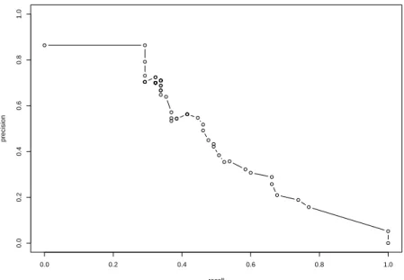
The PR curve is a diagram which plots precision (pre) against recall (rec) for different values of the threshold [30](see Figure 1.1 for a PR curve). In a network inference setting, this diagram illustrates the trade-off between re-turning a small amount of arcs (low recall due to high threshold) with high confidence (high precision) and returning many arcs (high recall) with low confidence (low precision).
1.1.2.2 F-Scores
The multicriteria nature of the inference problem can also be addressed by defining univariate measures which weight precision and recall. An example is given by the area under the PR-curve [2].
Another well-known measure is the F-score quantity [30] which is a weighted harmonic average of precision and recall:
Fβ(Tˆ(θ,W),T) =
(1+β2)(pre)(rec)
β2pre+rec (1.7)
whereβis a non-negative real parameter weighting the importance of recall versus that of precision. The F-score takes value in the interval[0, 1].
Three common values for the parameterβare
0.0 0.2 0.4 0.6 0.8 1.0
0.0
0.2
0.4
0.6
0.8
1.0
recall
precision
Fig. 1.1 Example of PR curves (generated with the R package ’minet’
• β=1: assigning equal weight to precision and recall
• β=2: (theF2-measure), which weighs recall twice as much as precision
• β = 0.5: (the F0.5-measure), which weighs precision twice as much as recall.
Note that in transcriptional network inference, precision is often valued higher than recall since the experimental cost to check for possible interac-tions is high.
A compact representation of the PR diagram can be returned by the maxi-mum and/or the average (avg)Fβ-score.
Fβmax(W,T) =maxθ Fβ(Tˆ(θ,W),T)
Fβavg(W,T) =avgθ Fβ(Tˆ(θ,W),T) (1.8)
whereθis the threshold parameter.
1.1.3
Causal Subset Selection
The inference of a network from data requires for each gene the identifica-tion of its own family of regulators. This problem is extremely complex since, givenn−1 variables inX−j, there is an exponential number 2n−1of candidate subsetsXSj.
An approach to solve this problem is given bycausal Bayesian networksthat provide a theoretical framework to identifying a causal subsetXSjof a variable Xj.
Definition 1.3 Xi is acauseofXj, denoted byXi → Xj, if there exists a value xi∈ Xisuch that settingXi =xileads to a change in the probability distribu-tion ofXj[24].
The definition of causality states that a causal relation between two vari-ables creates a stochastic dependency between the probability distributions of causes and effects. Thus, two causally linked variables are not independent and therefore the mutual information is larger than zero.
Xi↔Xj⇒I(Xi;Xj)>0 (1.9)
whereXi ↔Xjdenotes anundirected causal link, i.e.,Xi→XjorXi←Xj. Un-fortunately, since mutual information, unlike causality, is a symmetric mea-sure, it is not possible to derive the direction of an edge.
following we will keep on assuming thatcausality implies stochastic dependency.
However, the converse is not true, dependency does not imply causality
I(Xi;Xj)>0;Xi↔Xj. (1.10)
One counter-argument to the idea ofdependency implying causalityrelies on thecommon-cause effect. That is, a dependency between two variableXiandXj can be created by a common cause, i.e.,Xi ← Xk → Xj. These two variables can be dependent but manipulating one of them does not influence the other.
An illustration of this case is the well-known sentence “curing the symp-toms does not cure the disease”.
In this context, the definition of direct causality provides a solution to the problem of deriving causal dependency from stochastic dependency.
Definition 1.4 Xiis adirect causeofXjifXiis a cause ofXjand there is no other variableXksuch that once the value ofXkis known, a manipulation ofXi no longer changes the probability distribution ofXj[24].
This definition states that
if there are no sets of variables that cancel the dependency between two other variables, then one of the variables is a direct cause of the other.
In other words, it can be stated that if two variables are dependent in every context, then these variables have a causal relationship.
Once we make an additional assumption (known as causal sufficiency con-dition) the definition of direct cause provides the following implication in information-theoretic terms [6]:
∀XK⊆X−(i,j): I(Xi;Xj|XK)>0⇒Xi↔Xj (1.11)
The causal sufficiency condition requires that all variables that are causes to at least two effects (two variables in the dataset) be present in the set of mea-sured variables. Indeed, if there is a common cause to two observable effects, the two effects are dependent in every context except when conditioning on the common cause. If the common cause is hidden then (1.11) can lead to false conclusions about the causal relationships between the variables.
However, it should be noted that the causal sufficiency condition does not concern intermediate unidentified variables along the causal direction Xi → Xk→Xj, as illustrated by this example from [31].
There is a fundamental difference between having hidden variables along each edge in the causal direction and hidden variables that are common causes of several effects. Along a causal direction it is intuitive to accept that the causality between a grandparent and a grandson is preserved once the parent is removed. This corresponds to make an assumption ofcausal transitivity, that is
Xi→Xk Xk→Xj
⇒Xi→Xj.
However, if a common parent is missed and a link between a variable and its sibling is added, then such link is no longer causal since acting on the sibling does not change the distribution of the variable.
Hence, the causal sufficiency condition can be rephrased by assuming that there is no hidden common cause (to at least two effects)in the set of considered variables, i.e.,
∀(Xi,Xj)∈X, ∄(Xh∈/X): Xi←Xh→Xj (1.12)
The notions of information theory and causality introduced so far will be used in the rest of the chapter to present two main network inference ap-proaches which hold the attention of the bioinformatics community: i) meth-ods based on conditional mutual information that are able to infer a larger set of relationships between genes but at the price of a higher algorithmic complexity and ii) methods based on bivariate mutual information that infer undirected networks up to thousands of genes thanks to their low algorithmic complexity.
1.2
Inference Based on Conditional Mutual Information
Once causal sufficiency is assumed, the notion of conditional information al-lows the definition of a simple algorithm to infer an undirected network from observed data. The algorithm consists in
setting an undirect causal link between all couples(Xi,Xj)such that
∀XK⊆X−(i,j): I(Xi;Xj|XK)>0⇒Xi↔Xj
strategy adopted in constraint-based Bayesian network algorithms which will be briefly discussed in the following section.
1.2.1
Constraint-based methods
Algorithm 1: pseudo code of IC-algorithm
Start from an empty graph
foreachpair of variables(Xi,Xj)do
ifthere exists no subset XKin X−(i,j)such that I(Xi;Xj|XK) =0then set an edge connecting(Xi,Xj)
end end
Algorithm 2: pseudo code of the SGS algorithm
Start from the complete (fully connected) graph
foreachpair of variables(Xi,Xj)do
ifthere exists a subset XKin X−(i,j)such that I(Xi;Xj|XK) =0then remove the edge connecting(Xi,Xj)
end end
IC (Algorithm 1, [26]) and SGS (Algorithm 2, [31]) are two state-of-the-art contraint-based algorithms which infer the network by carrying out a set of conditional independence tests. Note that IC proceeds in a forward manner by starting with an empty graph while SGS proceeds in a backward manner by removing progressively edges from a fully connected graph. However in both algorithms, the IF instruction in the third line requires a computationally expensive procedure related to the search in the space of conditioning sets XK⊆X−(i,j). This means that, givennvariables, there are 2n−2potential sub-sets for each couple(Xi,Xj). In order to address this issue, the PC algorithm has been proposed by [26] to speed up the SGS algorithm by replacing the IF test with the pseudo code detailed in Algorithm 3. The rationale of the PC algorithm is to make conditional independence tests by using growing condi-tioning sets.
Algorithm 3: pseudo code of the subset search procedure in PC-algorithm
foreachsubset size going from|K|=0to|K|=n−2do foreachsubset of variables XKof size|K|do
ifI(Xi;Xj|XK) =0then
remove the edge connecting(Xi,Xj) quit the twoforloops
end end end
1.2.2
Approximated Conditional Mutual Information
In [37], the authors propose an information-theoretic translation of the PC al-gorithm that uses:
• a single conditioning variableXk instead of the set of variablesXK, re-placingI(Xi;Xj|XK)byI(Xi;Xj|Xk).
• two thresholdsθ1andθ2representing estimation biases in the indepen-dence tests.
Algorithm 4: pseudo code of [37]
Start from an empty graph
foreachpair of variables(Xi,Xj)do
if I(Xi;Xj)>θ1then
ifthere exists no variable Xkin X−(i,j)such that I(Xi;Xj|Xk)≤θ2then set an edge connecting(Xi,Xj)
end end end
withθ1andθ2thresholds (parameters) of the method
Both modifications of the PC algorithm render this method adapted to real microarray datasets.
1.2.3
Variable Selection Algorithms
inference by repeating a variable selection step in the spaceX−jfor each vari-able varivari-ableXj ∈X.
A generic information-theoretic objective of variable selection can be for-mulated as follows [22]:
Given an output variable Xj and n−1 input variables X−j , find the smallest subset XS ⊆X−jthat maximizes the mutual information I(XS;Xj)between inputs and output.
Note that maximizing the (mutual) information of a subset of variables is equivalent to reducing the uncertainty (entropy) of the target variable.
Using variable selection strategies for network inference has many practical and theoretical advantages [11, 32]. For instance:
1. Some variable selection algorithms, like filters, can deal with thousands of variables in a reasonable amount of time. This makes inference scal-able to large networks.
2. Variable selection algorithms may be easily executed in parallel, since each of thensubset selection tasks is independent.
3. Variable selection algorithms can use a priori knowledge. For example, knowing the list of regulator genes of an organism can improve the se-lection speed and the inference quality by limiting the search space of the selection step to a smaller list of genes.
Another advantage of a variable selection approach is that the subset that maximizes mutual information with the target contains all direct (causal) in-teractions [32].
The disadvantage is that this subset can also contain non-causal variables [32]. This results from theexplaining away effect.
Definition 1.5 [The explaining away effect] [24] Once the value of a common effect is given, it creates a dependency between its causes because each cause explains away the occurrence of the effect, thereby making the other cause less likely.
This is a common mechanism used by medical doctors when doing their diagnoses.
Example 2 Some cancer can cause headache but a lot of more probable diseases, such as a cold, can also cause headache. Once a doctor has evidence that headaches are caused by a cold, he stops searching for a cancer although having cold and having a cancer are two independent events (see Figure 1.2).
In information-theoretic terms, the explaining away effect can be expressed by a conditional mutual information higher than the mutual information [6, 12, 15]:
Xi→Xk ←Xj ⇒I(Xi;Xj|Xk)>I(Xi;Xj) (1.13)
This effect, is also known as negative interaction [13], complementarity [22] or synergy [1].
In order to avoid this problem, one should determine which of the selected variables are indirect links and eliminate them from the selection. This can be done by modifying properly the PC algorithm (Algorithm 3) and using it to explore, instead of the whole search spaceX−(i,j), the selected subsetXS[3]. It follows that the procedure is still exponential but in the size|S|of the subset selected.
1.3
Inference Based on Pairwise Mutual Information
This section will present a set of algorithms for inferring networks from ob-served data relying only on the computation of pairwise mutual information. In these methods, a link between two nodes is set if its corresponding score (based on pairwise mutual information) is higher than the chosen threshold.
All these methods require the computation of the mutual information ma-trix MIM= (mimij)i,j∈A, a square matrix whoseij-th element is given by,
mimij= I(Xi;Xj) (1.14)
This is the mutual information betweenXiand Xj, whereXi andXj are ran-dom variables denoting the expression level of theith/jth gene in a transcrip-tional regulatory network inference.
These methods have major advantages which enable them to deal with mi-croarray data:
Cancer Cold
Headache
• an affordable computational complexity. This results from the fact that only n2(n−1)computations of mutual information, based on bivariate probability distributions, are required to obtain the MIM [17].
• they do not require a large amount of samples, since only bivariate dis-tribution are to be estimated. Hence even basic entropy estimators per-form well with these methods [25]. Most of these methods can be tested using the Bioconductorminetpackage [21].
1.3.1
Relevance Network (RELNET)
The relevance network approach [5] has been introduced for gene clustering and successfully applied to infer relationships between RNA expression and chemotherapeutic susceptibility [4]. This method infers a network in which a pair of genes {Xi,Xj} is linked by an edge if the mutual informationI(Xi;Xj) is larger than a given thresholdθ. The complexity of the method isO(n2)since all pairwise interactions are considered.
This method relies on the assumptioncausality implies dependency(Section 1.1.3): Xi ↔Xj ⇒I(Xi;Xj)>0. However, it does not eliminate all indirect interac-tions between genes. For example, if geneX1regulates both geneX2and gene X3, this would cause a high mutual information between the pairs {X1,X2}, {X1,X3} and {X2,X3}. As a consequence, the algorithm will set an edge be-tweenX2andX3although these two genes interact only through geneX1.
Note that if one considers correlation instead of mutual information this approach boils down to building a correlation network [14].
1.3.2
Context Likelihood of Relatedness (CLR)
The CLR algorithm [9] is an extension of the RELNET algorithm. This al-gorithm derives a score from the empirical distribution of the mutual infor-mation for each pair of genes. In particular, instead of considering the in-formation I(Xi;Xj)between genesXi and Xj, it takes into account the score
wij= q
z2i +z2j where
zi=max
0, I(Xi;Xj)−µi
σi
(1.15)
Algorithm 5: pseudo code of the normal version of CLR algorithm
Input: I(Xi;Xj), ∀i,j∈A={1, 2, ...,n}
Output: the weighted adjacency matrixW(having elementswij)
foreachinput Xiin the input space Xdo
µi ←mean(I(Xi;Xj),j∈ {1, 2, ...,n})
σi←variance(I(Xi;Xj), j∈ {1, 2, ...,n})
end
foreachpair of variables Xi,jin the input space Xdo
wij←max
0,√1 2∗
nI(Xi;Xj)−µi σi +
I(Xi;Xj)−µj
σj
o
end
1.3.3
Chow-Liu Tree
The Chow and Liu approach consists in finding the maximum spanning tree on the complete graph whose edge weights are the mutual information be-tween two nodes [7].
In graph theory, a tree is a graph in which any two vertexes are connected by exactly one path. A spanning tree is a tree that connects all the vertexes of the graph. The maximum spanning tree is the spanning tree whose sum of edge weights is greater than or equal to that of every other spanning tree.
A maximum spanning tree can be computed inO(n2logn)using, for exam-ple, Kruskal’s algorithm [23]. The drawback of this method lies in the fact that the resulting network has typically a low number of edges. Also precision and recall cannot be studied as a function of a parameter.
1.3.4
The Algorithm for the Reconstruction of Accurate Cellular Networks (ARACNE)
ARACNE [17] is based on the Data Processing Inequality [8]. If geneXi inter-acts with geneXjthrough geneXk, thenI(Xi;Xj)≤min I(Xi;Xk),I(Xj;Xk)
. ARACNE begins by assigning to each pair of nodes a weight equal to their mutual information. Then, as in RELNET, all edges for which I(Xi;Xj) < θ are removed, withθa given threshold. Eventually, the weakest edge of each triplet is interpreted as an indirect interaction and is removed (see pseudo code Algorithm 6).
An extension of ARACNE removes the weakest edge only if the difference between the two lowest weights lies above a thresholdη. Hence, increasing
If the network is a tree including only pairwise interactions, the method guarantees the reconstruction of the original network, once it is provided with the exact MIM (see [17]). ARACNE’s complexity isO(n3)since the algorithm considers all triplets of genes. In [17] the method has been able to recover components of the transcriptional regulatory network in mammalian cells and has outperformed Bayesian networks and relevance networks on several in-ference tasks [17]. Chow-Liu tree is proved to be a subnetwork of the network reconstructed by the ARACNE algorithm [17].
Algorithm 6: pseudo code of ARACNE algorithm
Input: the MIM, i.e.,I(Xi;Xj),∀i,j∈ {1, 2, ...,n}
Output: the weighted adjacency matrixW(havingwijas elements)
foreachpair of variables Xi,jin the input space Xdo
foreachvariable Xkin the space X−(i,j)do
ifI(Xi;Xj)<θthen wij←0
else if(I(Xi;Xj)< I(Xi;Xk) and I(Xi;Xj)< I(Xj;Xk))then wij←0
else
wij←I(Xi;Xj)
end end end
1.3.5
Minimum Redundancy Networks (MRNET)
low informationI(Xi;Xk)to the previously selected variable. In the following steps, given a setXSof selected variables, the criterion updatesXS by choos-ing the variable which maximizes the MRMR score.
XiMRMR=arg max Xi∈X−(i,j)
I(Xi;Xj)− 1
|S|k
∑
∈SI(Xi;Xk) !(1.16)
At each step of the algorithm, the selected variable is expected to allow an efficient trade-off between relevance and redundancy. The network inference approach MRNET, consists in repeating this selection procedure for each tar-get geneXj ∈ X. For each pair{Xi,Xj}, MRMR returns two (not necessarily equal) scores si and sj according to (1.16). The score of the pair{Xi,Xj} is then computed by taking the maximum betweensiandsj. A specific network can then be inferred by deleting all the edges whose score lies below a given threshold θ(as in RELNET, CLR and ARACNE). Thus, the algorithm infers an edge between Xi and Xj either when Xi is a well-ranked predictor ofXj (si>θ), or whenXjis a well-ranked predictor ofXi(sj >θ).
An effective implementation of the greedy search based on a similarity ma-trix is given in [19]. This implementation demands anO(f×n)complexity for selecting f variables. It follows that MRNET has anO(f×n2)complexity since the variable selection step is repeated for each of thengenes. In other terms, the complexity ranges betweenO(n2)andO(n3)according to the value of f. In practice, the selection of variables is stopped when the average redun-dancy term |1S|∑k∈SI(Xi;Xk)exceeds the relevance termI(Xi;Xj).
Although MRNET is based on a variable selection strategy, it does not suf-fer from the explaining away effect as most variable selection methods (see Section 1.2.3): Xi→Xk←Xj ⇒I(Xi;Xj|Xk)>I(Xi;Xj). Indeed, the MRMR criterion only relies on pairwise interactions, hence it does not measure the increase in information due to conditioningI(Xi;Xj|Xk). Instead, it will con-sider the scoresi = I(Xi;Xj)−I(Xi;Xk)whereI(Xi;Xj) =0 sinceXiandXj are independent andI(Xi;Xk)>0 sinceXiis a cause ofXk(compare Example 1.2.3). This score si is negative andXi will be badly ranked by MRMR. The same will happen for rankingXjas a predictor ofXi.
Several papers [16,20,25,29] have experimentally shown the accuracy of the MRNET method both in simulated and real data network inference tasks.
1.4
Arc Orientation
Algorithm 7: Detailed pseudo-code of the MRNET algorithm (given the MI M).
Input: a matrix of weights MIM (with elementsI(Xi;Xj)) of sizen
Output: the weighted adjacency matrixW
Initialize the weighted adjacency matrixWton×nzeros
foreachvariable j∈ A={1, 2, ...,n}do
Initialize search space:R←A\ {j} Initialize selected variable:S←∅
Initializerelevancevector:relevancej ←I(Xi;Xj),i∈R Initializeredundancyvector:redundancyj←0,i∈R
whilewkj>0do
Select best variable:k←arg maxi∈R(relevancei−redundancyi/|S|) Update subset :S← {S,k}
Update matrix:wkj ←relevancek−redundancyk/|S| Update search space :R←R\k
Updateredundancyvector:
redundancyi←redundancyi+I(Xi;Xk),i∈R
end end
question is positive. This can be done in some cases thanks to the previously seen explaining away effectXi →Xk←Xj⇒I(Xi;Xj|Xk)>I(Xi;Xj).
Let us first remark that because of the following equality
I(Xi;Xj)−I(Xi;Xj|Xk) =I(Xi;Xk)−I(Xi;Xk|Xj) =I(Xj;Xk)−I(Xj;Xk|Xi) (1.17)
the reversal statement of (1.13) is not necessarily true,
I(Xi;Xj|Xk)>I(Xi;Xj);Xi →Xk←Xj
since I(Xi;Xj|Xk) > I(Xi;Xj) could also imply Xk → Xi ← Xj or Xi → Xj ←Xk. Notwithstanding, given particular configurations of the undirected network, arcs can be oriented thanks to the explaining-away effect. This can be done in two ways:
First, if the variableXkis linked toXiandXj, and an explaining away effect between them has been detected, then the variableXk is a common effect of the two other variables. More formally,
Xi↔Xk ↔Xj I(Xi;Xj|Xk)>I(Xi;Xj)
Second, if the variableXkis a consequence ofXiand is linked toXjand no explaining away effect occurs between them, thenXjis a consequence ofXk:
Xi→Xk ↔Xj I(Xi;Xj|Xk)≤I(Xi;Xj)
⇒Xi→Xk→Xj (1.19)
The two rules (1.18) and (1.19) are an information-theoretic translation of the arc orientation criteria used in [26, 31].
Note that the explaining away effect Xi → Xk ← Xj ⇒ I(Xi;Xj|Xk) > I(Xi;Xj)is true in general, but not always. Consider the following example:
Example 3 Disease A can cause the skin covered by eczema and disease B can cause the skin have wounds. Let the variable S (skin), have three possible values (eczema, wounds, normal). Although disease A and B are two causes of skin injuries S, there is no more information brought by an evidence in favor of one of the diseases than the information already given by the state of the skin.
This example illustrates that, in order to observe an explaining away effect, the two causes should have the same effect on the same target variable [24].
Although directed cycles can represent feed-back and feed-forward effects, there is no suitable joint probability to model these situations. Distributions such as p(A|B)p(B|C)p(C|A)are not well defined probability distributions, apart from very special cases [34]. Furthermore, the notion of loops is related to dynamics whereas the probability distribution modeled here comes from samples with no temporal dependencies. Hence, a third rule commonly used to orient arcs in a partially oriented network consists in removing cycles in triplets of variables [18].
In order to guarantee a correct inference of an oriented network, additional as-sumptions are required. Commonly, the causal Markov and the causal faith-fulness assumptions are made [26, 31]. These two properties are defined as follow.
Definition 1.6 Thecausal Markov conditionholds if every variable is statistically independent of its non-effects conditional on its direct causes.
Definition 1.7 Thefaithfulness conditionholds if the only existing conditional independencies are those specified by the causal Markov condition.
Note, that these two conditions include the assumptions defined above such as causality implies dependency or causal transitivity (for a detailed analysis of these assumptions see [35].)
1.4.1
Assessing arc orientation methods
Algorithm 8: pseudo code of SGS/IC arc orientation step for conditioning sets of size one
foreachtriplet Xi ↔Xk↔Xjwith no link connecting Xi↔Xjdo I(Xi;Xj|Xk)>I(Xi;Xj)⇒Xi→Xk ←Xj
end
while there remain undirected edges, orient edges subject todo
avoiding new colliders avoiding cycles
end
Algorithm 9: pseudo code of the “remove cycles” step of [3] algorithm
compute the list of cycles in the graph
while there exists cycles in the graphdo
reverse edge that belongs the highest amount of cycles update the list of cycles
end
of correctly oriented arcs, the ones which are oriented in the wrong direction and those arc which have not been oriented at all. Depending on the prob-lem, different strategies are applied in the literature. If one is interested in the overall performance, the number of correctly oriented arcs is compared to the number of wrongly oriented arcs. The problem with this method is, that the more arcs are oriented, the less significant the orientation is (due to the de-creasing score of a arc). Another evaluation possibility is a weighted matrix, which is interesting when searching for the directionalities in a local network, e.g. the arcs in a certain “neighborhood” of the target variable. In this case, the orientation of arcs close to the target can be higher rated than that of arcs further away.
original network. Precision and recall are then defined as follows
rec= |tp|+
|ptp| 2
|f n|+|p f n2 |+|tp|+|ptp2 | (1.20)
pre= |tp|+
|ptp| 2
|f p|+|p f p2 |+|tp|+|ptp2 | (1.21)
Summary
Transcriptional network inference aims at representing interactions between transcription factors and regulated genes with a graph. Most methods intro-duced in this chapter are able to distinguish between dependency (e.g. cor-regulated gene) and causality (e.g. transcription factor) by relying on assump-tions such as causality implies dependencyor causal sufficiency. Among infer-ence methods based on information theory, mutual information networks, re-lying on the matrix of pairwise mutual information, are particularly adapted to large number of variables and low number of samples typically encoun-tered in microarray data. However, these methods only infer an undirected graph. In order to orient the arcs, a second step is required such as meth-ods based on the explaining away effect. Finally, validation measures such as PR-curves and F-scores have been introduced here in order to assess inferred networks. Many tools and algorithms introduced in this chapter can be tested using the Bioconductor packageminet.
Bibliography
1Dimitris Anastassiou. Computational analysis of the synergy among multiple interacting genes. Mol Syst Biol, 3, Febru-ary 2007.
2Sahely Bhadra, Chiranjib Bhattacharyya, Nagasuma R Chandra, and Saira Mian. A linear programming approach for es-timating the structure of a sparse linear genetic network from transcript profiling data.Algorithms for Molecular Biology, 4:5+, February 2009.
3Facundo Bromberg and Dimitris Margari-tis. Improving the reliability of causal discovery from small data sets using ar-gumentation. Journal Machine Learning Research, 10, 2009.
4A. J. Butte, P. Tamayo , D. Slonim, T.R. Golub, and I.S. Kohane. Discovering functional relationships between RNA expression and chemotherapeutic suscep-tibility using relevance networks. Pro-ceedings of the National Academy of Sciences, 97(22):12182–12186, 2000.
5A. J. Butte and I. S. Kohane. Mutual in-formation relevance networks: Functional genomic clustering using pairwise en-tropy measurments. Pacific Symposium on Biocomputing, 5:415–426, 2000.
7C. Chow and C. Liu. Approximating discrete probability distributions with de-pendence trees. Information Theory, IEEE Transactions on, 14, 1968.
8T. M. Cover and J. A. Thomas.Elements of Information Theory. John Wiley, New York, 1990.
9J.J. Faith, B. Hayete, J.T. Thaden, I. Mogno, J. Wierzbowski, G. Cottarel, S. Kasif, J.J. Collins, and T.S. Gardner. Large-scale mapping and validation of escherichia coli transcriptional regulation from a com-pendium of expression profiles. PLoS Biology, 5, 2007.
10T. S. Gardner and J. Faith. Reverse-engineering transcription control net-works.Physics of Life Reviews 2, 2005. 11K. Hwang, J. W. Lee, S. Chung, and
B. Zhang. Construction of large-scale bayesian networks by local to global search. In7th Pacific Rim International Conference on Artificial Intelligence, 2002. 12A. Jakulin and I. Bratko. Quantifying and
visualizing attribute interactions, 2003. 13A. Jakulin and I. Bratko. Testing the
sig-nificance of attribute interactions. InProc. of 21st International Conference on Machine Learning (ICML), pages 409–416, 2004. 14B. H. Junker and F. Schreiber. Analysis
of Biological Networks. Bioinformatics. Wiley-Interscience, 2008.
15K. Liang and X. Wang. Gene regulatory network reconstruction using conditional mutual information. EURASIP Journal on Bioinformatics and Systems Biology, 2008. 16F. M. Lopes, D. C. Martins, and R. M.
Ce-sar. Comparative study of grns inference methods based on feature selection by mutual information. InIEEE International Workshop on Genomic Signal Processing and Statistics, 2009.
17A. A. Margolin, I. Nemenman, K. Basso, C. Wiggins, G. Stolovitzky, R. Dalla Fav-era, and A. Califano. ARACNE: an algo-rithm for the reconstruction of gene regu-latory networks in a mammalian cellular context.BMC Bioinformatics, 7, 2006. 18C. Meek. Strong completeness and
faith-fulness in Bayesian networks. In Proceed-ings of Eleventh Conference on Uncertainty in Artificial Intelligence,Montreal, QU, pages 411–418. M. Kaufmann, August 1995.
19P. Merz and B. Freisleben. Greedy and local search heuristics for unconstrained binary quadratic programming. Journal of Heuristics, 8(2):1381–1231, 2002.
20P. E. Meyer, K. Kontos, F. Lafitte, and G. Bontempi. Information-theoretic in-ference of large transcriptional regulatory networks. EURASIP Journal on Bioinfor-matics and Systems Biology, Special Issue on Information-Theoretic Methods for Bioinformatics, 2007.
21P. E. Meyer, F. Lafitte, and G. Bontempi. Minet: An open source r/bioconductor package for mutual information based network inference. BMC Bioinformatics, 2008.
22P. E. Meyer, C. Schretter, and G. Bontempi. Information-theoretic feature selection using variable complementarity. IEEE Journal of Special Topics in Signal Processing, 2(3), 2008.
23B. M. E. Moret and H. D. Shapiro. An empirical analysis of algorithms for con-structing a minimum spanning tree. In Springer, editor,Lecture Notes in Computer Science, volume 519, 1991.
24R. E. Neapolitan. Learning Bayesian Net-works. Prentice Hall, 2003.
25C. Olsen, P. E. Meyer, and G. Bontempi. On the impact of missing values on tran-scriptional regulatory network inference based on mutual information. EURASIP Journal on Bioinformatics and Systems Biol-ogy, 2009.
26J. Pearl. Causality: Models, Reasoning, and Inference. Cambridge University Press, 2000.
27H. Peng, F. Long, and C. Ding. Feature se-lection based on mutual information: cri-teria of max-dependency, max-relevance, and min-redundancy. IEEE Transactions on Pattern Analysis and Machine Intelligence, 27(8):1226–1238, 2005.
28C. E. Shannon. A mathematical theory of communication. Bell System Technical Journal, 1948.
30Marina Sokolova, Nathalie Japkowicz, and Stan Szpakowicz. Beyond accuracy, f-score and roc: a family of discriminant measures for performance evaluation. InProceedings of the AAAI’06 workshop on Evaluation Methods for Machine Learning, 2006.
31P. Spirtes, C. Glymour, and R. Scheines. Causation, Prediction, and Search. MIT Press, 2001.
32I. Tsamardinos, C. Aliferis, and A. Stat-nikov. Algorithms for large scale markov blanket discovery. InThe 16th International FLAIRS Conference, 2003.
33E. P. van Someren, L. F. A. Wessels, E. Backer, and M. J. T. Reinders. Genetic network modeling. Pharmacogenomics, 3(4):507–525, 2002.
34J. Whittaker. Graphical Models in Applied Multivariate Statistics. Wiley, 1990. 35J. Zhang and P. Spirtes. Detection of
un-faithfulness and robust causal inference. Minds Mach., 18(2):239–271, 2008. 36Xin Zhang, Chitta Baral, and Seungchan
Kim. An algorithm to learn causal re-lations between genes from steady state data: Simulation and its application to melanoma dataset.Artificial Intelligence in Medicine, pages 524–534, 2005.