Reasoning From Point Clouds
CPE Senior Project
California Polytechnic State University, San Luis Obispo
1 Introduction
2 Problem Statement 3 Preparation
4 Hardware 5 Software
5.1 Object Counting Architecture 5.2 Object Detection Architecture 5.3 Libraries
5.4 Overfitting 5.5 Setup 6 Results
Chapter 1 INTRODUCTION
Due to technological improvements to computers in computation speed and power, many futuristic engineering feats are becoming possible. Autonomous robots are computationally heavy and rely on complex algorithms and deep learning to reason about their environment and make decisions. In the past decade, advancements in computers have made dreams of self-driving cars and automated jobs a reality, since computations can now be done quickly enough for these robots to safely operate. Self-driving vehicles have the potential to enable restricted individuals to live fuller lives, reduce unnecessary death, decrease busy time, and enable more revolutionary applications utilizing the same technology. Although most car companies are researching and developing self-driving cars with the help of top universities, many challenges still face the industry. Some of the top challenges facing the industry today include measuring driver awareness and readiness to take over, balancing cost and performance of sensors, reasoning about the environment, and collaboration between vehicles.
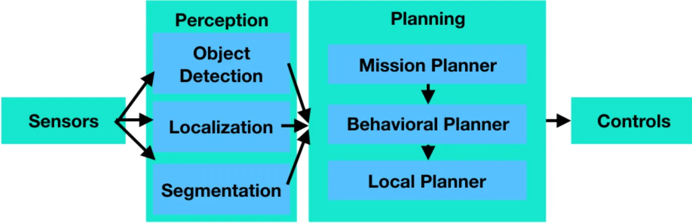
Figure 1: Simple Autonomous Robot Software Stack
Tech in the 2007 DARPA Grand Challenge[1]. The software stack is divided into four main parts: sensors, perception, planning, and controls. Although modern software for autonomous vehicles is more complicated and includes more features and steps including feedback loops, the fundamentals still hold.
Self-driving cars generally use cameras, stereo cameras, LIDAR, radar, ultrasonic, GNSS, IMU, and odometer sensors. Each sensor has a unique purpose and tradeoffs. Cameras are essential and can be combined using disparity maps to enable depth estimation. LIDAR consists of spinning lasers used to generate a detailed 3D scene point cloud. Radar and ultrasonic sensors are used for distance measurement and object detection in adverse environments. GNSS and IMU are used together to measure the heading of the ego vehicle, and a wheel odometer is used to calculate overall speed and orientation. LIDAR is generally considered essential due to it's ability to get an accurate 3D representation of the surrounding environment in all weather regardless of lighting or precipitation.
fusing sensor data and prediction the ego vehicle's current 3D positon, 3D velocity, and 4D orientation. Kalman filters use a prediction and correction model to predict how the vehicle's state evolved since the last time step including error propagation, and update based on measurements. Another major feature of perception is object detection, which involves identifying dynamic objects in the environment and estimating their location and size via a bounding box. In 2D, this can be done using convolutional neural networks again, but is much more difficult in 3D.
PROBLEM STATEMENT
Over the past two years, 3D object detection has been a major area of focus across industry and academia. This is primarily due to the difficulty of learning data from point clouds. While camera images are fixed size and can therefore be easily trained on using convolution, point clouds are unstructured series of points in three dimensions. Therefore, there is no fixed number of features, or a structure to run convolution on. Instead, researchers have developed many ways of attempting to learn from this data, however there is no clear consensus on what is the best method, as each has
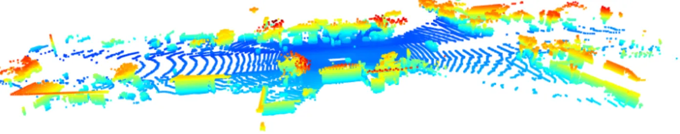
advantages and disadvantages. Figure 2 shows an example point cloud from the Waymo Open Dataset, discussed later, visualized in colors using Open3D.
Figure 2: Example Point Cloud from Waymo Open Dataset Some of the main techniques for learning 3D data from point clouds are
as input and use a fully connected network on each point individually, then a
permutation-invariant max pooling layer to aggregate global information[3]. Many of these papers, and their implementations in TensorFlow or PyTorch, can be found online in a GitHub repository[4].
Since 3D object detection is a difficult task, there are many publicly available datasets, most notably the KITTI Vision Benchmark Suite[5]. At the end of August, Waymo
released a 20 terabyte driving dataset to help researchers in the task of 3D object detection using point clouds[6]. Although there are several large data sets available, there isn't enough data to accurately predict performance on roads, so researchers often test using simulators. While simulators can offer benefits to training models, they aren't an accurate representation of real-life scenarios, leading to potential difficulties when transitioning a model to the real world.
PREPARATION
This project required a lot more knowledge than is taught at an undergraduate level. I gained precursory knowledge into data science and autonomous robotics through courses at Cal Poly, then went online to learn more about the current state and fields of the industry. I took classes online through Coursera, an online learning platform
founded by Stanford deep learning and robotics professor Andrew Ng, including specializations in Machine Learning, Deep Learning, Self-Driving Cars, TensorFlow, and Probabilistic Graphical Models. Each of these specializations was packed with approximately 6 months worth of material, and were taught by experts at universities including Stanford and Toronto. These
classes gave me the background knowledge needed to understand research papers and implement my own projects, and recommended research papers to look into. I gained insight into the state of robotics through podcasts including Artificial
Chapter 4 HARDWARE
For this project, I used an Apple iMac desktop with 8 GB RAM. This limited the size of the deep learning architecture I could use, and the amount of driving segments I could use at each moment during training. My computer only had one GPU as well, which made training slower than in the VoxelNet paper. While the paper used a voxel length and width of 0.2m, I used a length and width of 2m due to the capabilities of my
SOFTWARE 5. 1 Object Counting Architecture
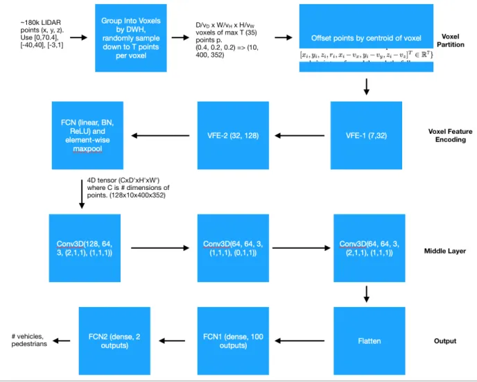
The neural network architecture for this project was a smaller, modified version of VoxelNet. A diagram of the architecture used for the task of object counting can be seen in figure 3. The goal of this network was to count the number of vehicles and pedestrians in a scene, a simpler task of recognizing objects in point clouds.
Figure 3: Modified VoxelNet Architecture
Point clouds from the Waymo Open dataset consisted of approximately 180,000
from -40 to 40 m, and z coordinates ranging from -3 to 1 m. The first step was to group the points into equally distributed voxels. For this project, I used voxels of size 2
meters by 2 meters. For voxels with over T points, points were then randomly sampled down to T points. In training, I used 10 points for T. In the final step of voxel
partitioning, points were offset by the centroid of each voxel, calculated as an average of the T points within the voxel, to obtain a 7 dimensional vector per point.
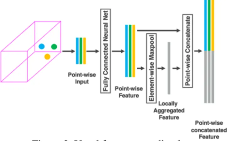
Points were then fed into the Voxel Feature Encoding (VFE) layer, which included two VFE blocks used to upsample the amount of features per point to 32, then 128. A diagram of the VFE block, taken from the VoxelNet paper, can be seen to the right in Figure 4. The VFE block
begins with a fully connected network (FCN) which learns a matrix of size cin x (cout/2). The point-wise features from this layer are then fed into an element-wise Maxpool, used to capture the maximum value from all points over each dimension. Pooling layers are used to provide translation invariance, and max pooling extracts the sharpest features of the input. The output of the FCN and Maxpool layers are then aggregated and normalized with a batch-norm layer. After both VFE layers, another FCN, batch normalization (BatchNorm), and Maxpool layer is applied to obtain a 4D tensor of size CxTxH'xW', where C is the number of features per point.
Each 3D convolution block applies 3D convolution, normalization using BatchNorm, and a rectified linear unit activation function. The parameters shown in figure 3 are the number of input and output channels, kernel size, stride size, and padding for the 3D convolutions. These layers are used to aggregate and expand upon voxel-wise features.
Once features have been learned, they are fed into the output layer. Figure 3 shows the output layer used for the task of object counting. This layer consisted of three steps. The first step was to flatten all inputs into a single feature array, so that the features could be fed into FCN layers. The features were then downsampled through FCN layers to 100 features, and finally to the two outputs, vehicle and pedestrian counts. Loss was calculated using mean squared error from the Waymo training data.
5.2 Region Proposal Architecture
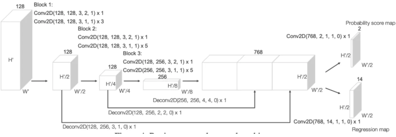
Region proposal is a much more difficult task, and involved replacing the output layer with a region proposal network (RPN). The RPN uses a modified Faster R-CNN[9]. The architecture for the RPN layer is detailed in figure 5, taken from the VoxelNet paper. It's implementation is from an open source GitHub project[10], which provided all the
convolution layers, to generate a probability score map and regression map. The probability score map contained the probability that each voxel belonged to a positive or negative anchor, while the regression map contained the proposed 7D dimensions for the object.
Figure 5: Region Proposal Network
Loss for the RPN was calculated as the sum of binary cross entropy over positive anchor probabilities, negative anchor probabilities, and regression output.
5.3 Libraries
Chapter 6 RESULTS 6.1 Data
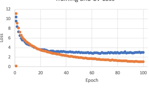
The object counting model worked surprisingly well on the Waymo Open Dataset, considering the memory constraints on the model. Although there were only 1/100th the number of Voxels as VoxelNet used, mean squared error (MSE) of vehicles and pedestrians approached 1.5 on the cross validation set. This is plotted in figure 6 below, which shows the CV set and training set error before and after regulation. As is clearly visible, the model overfit the data quickly, as no improvements were seen after 100 epochs on the CV set without regularization. While the training set error kept improving, the CV set error became stagnant. This was improved slightly by adding L2 regularization, which penalizes updates to weights using a squared parameter.
including a significant decrease in error on the CV set. The MSE approached 0.65, less than half of the error before regularization. MSE heavily punishes large differences in estimations, since it squares any error, showing that the model tightly fit the Waymo data. There was a lot of room for error, as a single scene typically ranged had 10 to 50 of each type of object.
Once it was clear that the CV set wasn't improving, the model stopped training to avoid severe overfitting. The model was then loaded into a Python script connected to the Carla API, and was fed live data in the form of point clouds. The setup can be seen in figure 7, which shows the image seen in the Carla simulator towards the right, and some of the calculations to the left. While the calculations were sometimes correct, the model was very off in a lot of cases, predicting negative numbers which should never occur. Although the model worked very well on scenes from the Waymo Open Dataset, which it was trained on, it struggled when transitioning to the Carla simulator. This suggests that the point cloud data obtained from the Carla simulator didn't correlate to the real driving data in scenes from the Waymo Open Dataset. This is possibly due to different driving environments, lower resolution on point clouds, or different
representations of objects confusing the model. Convolutional neural networks learn features by recognizing patterns in the images, so it's possible that the simulator
Figure 7: Model Running with Carla
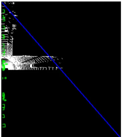
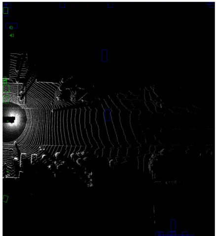
Next, the output layer was stripped and replaced with a region proposal network. The region proposal network didn't perform very well on the data, again most likely due to the small number of voxels. The calculations for region proposal and their Python implementations were taken from open source software, so they were most likely correct. Although loss decreased, the bounding box predictions were very large and didn't seem to correlate with the data. An example is shown in figure 8, where the ground truth boxes are shown in green and a predicted box is shown in blue from a bird's eye view. The predicted boxes had absurd values including many 0's, infinities, high values, and NaN's, suggesting that the model was failing to predict the data somewhere along the pipeline. As the calculations for bounding boxes were taken from an open source, verified implementation, it's more likely that the error was in the
and variance. The ability of the model to fit the data could be improved by making the model more complex, and the effects of overfitting could be negated by increasing the training set size (the Waymo Open Data set has many more segments to train on), augmenting data as in the VoxelNet paper, and increasing the effects of regularization.
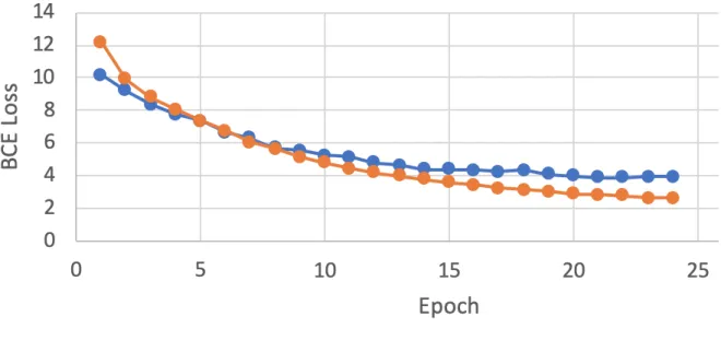
Figure 9: RPN Training Loss
During Thanksgiving break, I got access to a much more powerful computer to train my model on. This gave me a chance to decrease the voxel size from 2m length and width to 0.5m, an increase in 16 times the number of voxels, although still significantly less than in the VoxelNet research paper. This caused major improvements in my
changing any parameters.
Figure 10: Training With More Voxels
power. With the Waymo Open Dataset being publicly available, performance could be improved over the KITTI dataset due to the magnitude of data now available for research. My limiting factor was training time and memory, since training for just 100 epochs took multiple days.
Figure 11: Example Point Cloud
6.2 Future
Future work would be useful to investigate how the strength of the model grows with voxel width and length. As voxel width and length shrink, the model would be expected to better fit the data, especially in the case of region proposal. My desktop only had 8 GB of RAM available, so I was limited in how many voxels I could use. Research papers publish results for highly optimized versions of their models, so a hyper-parameter search could be conducted to identify the optimal configuration for
Chapter 7 CONCLUSION
The goal of this project was to learn more about autonomous robots, perception, and examine the ability of simulators to model real-life scenarios. All of these goals were accomplished by taking classes and building projects, reading research papers, and closely analyzing and building VoxelNet, in addition to some unintended results. Through working on this project, I gained a much deeper understanding of the difficulties when working with large amounts of data under tight restrictions, the
REFERENCES
1. Reinholtz, Charles. “DARPA Urban Challenge Technical Paper.” Virginia Tech. DARPA, 13 Apr. 2007.
2. Simonyan, Karen, and Andrew Zisserman. “Very Deep Convolutional Networks For Large-Scale Image Recognition.” ICLR 2015, 10 Apr. 2015.
3. AXiong, Yuwen, et al. “Deformable Filter Convolution for Point Cloud Reasoning.” Uber ATG and University of Toronto. ArXiv, July 2019.
4. Yochengliu. “Awesome Point-Cloud Analysis.” GitHub, https://github.com/ Yochengliu/awesome-point-cloud-analysis.
5. The KITTI Vision Benchmark Suite, http://www.cvlibs.net/datasets/kitti/. 6. “Open Dataset.” Waymo, https://waymo.com/open/.
7. Zhou, Yin, and Oncel Tuzel. “VoxelNet: End-to-End Learning for Point Cloud Based 3D Object Detection.” 2018 IEEE/CVF Conference on Computer Vision and Pattern Recognition, 2018, doi:10.1109/cvpr.2018.00472.
8. Team, CARLA. “CARLA.” CARLA Simulator, http://carla.org/.
9. Ren, Shaoqing, et al. “Faster R-CNN: Towards Real-Time Object Detection with Region Proposal Networks.” ArXiv, 4 June 2015.