Robustifying trial-derived optimal
treatment rules for a target population
Ying-Qi Zhao∗
Public Health Sciences Division, Fred Hutchinson Cancer Research Center, Seattle, WA, 98109
e-mail:[email protected]
Donglin Zeng
Department of Biostatistics, University of North Carolina at Chapel Hill, Chapel Hill, NC, 27599
e-mail:[email protected]
Catherine M. Tangen and Michael L. Leblanc
Public Health Sciences Division, Fred Hutchinson Cancer Research Center, Seattle, WA, 98109
e-mail:[email protected];[email protected]
Abstract: Treatment rules based on individual patient characteristics that are easy to interpret and disseminate are important in clinical practice. Properly planned and conducted randomized clinical trials are used to con-struct individualized treatment rules. However, it is often a concern that trial participants lack representativeness, so it limits the applicability of the derived rules to a target population. In this work, we use data from a single trial study to propose a two-stage procedure to derive a robust and parsimonious rule to maximize the benefit in the target population. The procedure allows a wide range of possible covariate distributions in the tar-get population, with minimal assumptions on the first two moments of the covariate distribution. The practical utility and favorable performance of the methodology are demonstrated using extensive simulations and a real data application.
Keywords and phrases:Primary Minimax linear decision, biased sample, classification, individualized treatment rules, personalized medicine.
Received January 2018.
Contents
1 Introduction . . . 1718
2 Methodology . . . 1719
2.1 Background and the optimal treatment rule . . . 1719
2.2 A General Quality Value of Treatment Rules for the Target Pop-ulation . . . 1721
2.4 Estimating robust rules using empirical data . . . 1724
2.5 Choices of (ν, ρj) . . . 1726
3 Theoretical results . . . 1726
4 Simulation Studies . . . 1727
5 Data Analysis . . . 1730
6 Discussion . . . 1734
A Appendix . . . 1735
Acknowledgments . . . 1740
Supplementary Material . . . 1741
References . . . 1741
1. Introduction
In the new era of personalized medicine, it has been advocated that treat-ments should be recommended according to individual patient characteristics to account for considerable heterogeneity among patients’ responses to differ-ent treatmdiffer-ents (Hayes et al., 2007; Hamburg and Collins, 2010). Randomized clinical trials (RCTs) are ideal for constructing such rules, since they provide internal validity by ensuring consistency, positivity and no unmeasured con-founders (Greenland,1990; Hern´an and Robins,2006) that may be violated in observational studies.
Sophisticated statistical methods have been developed to estimate optimal individualized treatment rules using data from randomized trials. Regression-based methods estimate outcome as a function of patient covariates and treat-ment, and then select the treatment that maximizes the predicted outcome for each individual (Brinkley et al., 2010; Qian and Murphy, 2011; Kang et al.,
2014). Some recent developments directly search for the individualized treat-ment rules that maximize the benefit for future patients (Zhang et al., 2012; Zhao et al.,2012). When the primary outcome of interest is survival time sub-ject to right censoring, some methods have been proposed in this regard using either regression-based methods (Goldberg and Kosorok, 2012; Huang et al.,
2014) or direct search methods (Zhao et al.,2015).
The derived optimal rules sometimes are complex and nonlinear, so they are highly variable and may not be practically useful. To better inform clinical prac-tice, it is more desirable that a recommended treatment rule be easy to interpret and disseminate. As suggested in Orellana et al. (2010), the class of practically enforceable candidate regimes is significantly smaller than the class of arbitrary functions of covariates. Usually these regimes are comprised of functions that only depend on a small set of covariates, and are indexed by a set of finite di-mensional parameters. Statistically, Qian and Murphy (2011) used a rich linear basis for better modeling the outcome, with a sparsity penalty imposed to pre-serve the parsimoniousness of the resulting rule, while most works considered and recommended rules from a linear functional class.
partic-ipants differs from the one in a target population (Buchanan et al., 2016). A parsimonious treatment rule constructed from trial data using current methods cannot be directly carried over to a target population, when the population char-acteristics are different between the two. Some attempts have been made to ad-just population difference using inverse probability-of-selection weight method (Cole and Stuart, 2010). This, however, requires complete knowledge of pop-ulation selection mechanism, and it is yet to be extended to the context of developing optimal treatment rules.
In this paper, we aim to robustify the treatment rule from a trial so that the robustified rule is (1) parsimonious (linear in patient features in particular); (2) still maximizes a general benefit criterion when applied to the target popula-tion. We provide a new framework, called minimax linear decision (MiLD), to robustify the treatment rule. MiLD enables the construction of a linear rule that optimizes the general benefit function in the target population, allowing differ-ences between the target and the trial populations in the means and covariances in treatment effect modifiers. It can be further extended to construct nonlinear rules using the ‘kernel trick’, which avoids the explicit feature mapping but only relies on a kernel function to learn a nonlinear decision boundary. Regardless, MiLD requires no further assumptions beyond the first two moments of the covariate distributions. Moreover, our developed framework is applicable to all types of outcomes.
The remainder of the paper is organized as follows. In Section 2, we for-mulate the problem of finding a robust and parsimonious treatment rule using data from a clinical trial. The proposed method, MiLD, is then developed to optimize a general benefit function in the target population, allowing the covari-ate distribution to be different between the two populations. Consistency and convergence rate results are established for the proposed method. We present simulation studies to evaluate performances of the proposed method in Section
4. We further illustrate the method using a data example from a US NIH funded SWOG trial on castration-resistant prostate cancer patients in Section 5. The proofs of theoretical results are given in the Appendix.
2. Methodology
2.1. Background and the optimal treatment rule
LetT denote the outcome of interest,A∈ {−1,1} denote a binary treatment, and X = (X1, ..., Xm) ∈ Rm denote patient covariates. We assume the
in the trial population to receive treatment according tod. We denote this quan-tity asV(d), which is also called the value function ofd. The optimal treatment regimed∗ maximizesV(d) over all possibled. We assume that in the trial,
(A1) P(A=a|X)>0 with probability one for a∈ {−1,1};
(A2) {T(−1), T(1)}are independent ofAconditionalX;
(A3) consistency so that T(a) =aI(A=a)T.
Since V(d) = E{T(d)} = EX(E[T{d(X)}|X}]), where the outer expectation
EX(·) is taken with respect to the marginal distribution of X in the trial
population, the optimal treatment for any patient with characteristics x is d∗(x) = argmaxa∈{−1,1}E{T(a)|X = x} when there is no restriction of the functional form of the rule. These assumptions are typically standard and sat-isfied in randomized clinical trials (Robins et al.,2000), because application of the intervention to any individual is under the control of the investigator. This is however, not guaranteed in observational studies. For example, consistency assumption can be violated given that there could be variations of treatment, and each of them may have a different causal effect on the outcome. In addition, noncom- pliance can be severe in observational studies, where some subjects may never take what they are asked to take. If (A1)-(A3) are satisfied, the optimal treatment rule is
d∗(x) = sign{f∗(x)}, wheref∗(x) =E(T|X =x, A= 1)−E(T|X =x, A=−1).
To assess the overall benefit of the obtained rule when applied to the target population, we let pX(x) denote the distribution of X in the trial population,
and qX(x) denote the distribution of X in the target population, which is not
necessarily the same aspX(x). Furthermore, we assume
(A4) the support of qX(x) is contained in the support of pX(x), i.e., there is
no under-coverage in the trial study;
(A5) the potential outcome mean givenX is the same between the trial popu-lation and the target popupopu-lation. Thus, the treatment works the same in both populations.
Thus, the only difference between the two populations is due to the covariate distributions. LetPq denote the distribution ofX in the target population and
Ppdenote the distribution ofX in the trial population. LetEdenote the
expec-tation is taken with respect to the distribution of X in the target population. Under (A4) and (A5), it is easy to observe that the expected outcome of rule d(X) for the target population is
V(d) = E[T {d(X)}] =
E[T{d(X)}|X]dPq
=
E[T{d(X)}|X]dP
q
dPpdP p=E
X
E[T{d(X)}|X]qX(X) pX(X)
,
where EX[·] denotes the expectation under X ∼pX(x). Consequently, the
2.2. A General Quality Value of Treatment Rules for the Target Population
We propose a general criterion assessing the quality of a decision rule for the target population, which includes both the value function and the correct al-location rate to the optimal rule as special cases. For a given rule d(X), the proposed quality assessment in the target population is defined as
B(d) =E[W (X)I{d(X) =d∗(X)}],
where W(X) is a non-negative function, essentially a reward if the treatment ruled(x) is the optimal.
The quality value in the definition has a different interpretation depending on the choice ofW(x). For example, letW(x) =W1(x) =E{T|A=d∗(x), X=
x} −E{T|A = d∗(x), X = x} = |f∗(x)|. That is, for subject with covariate X = x, W(x) is the gain if he/she follows treatment rule d∗. B(d) achieves optimal ifd=d∗. This is becauseB(d) =V(d)+E{T(−d∗)}. Hence, maximizing
B(d) is equivalent to maximizing the value function in the target population. If we set W(X) = W2(X) ≡ 1, then B(d) = P{d(X) = d∗(X)}, and the
criterion corresponds to the correct allocation rate of the optimal treatment. Additionally, in practice,W(X) could allow more general trade off between the benefit of optimal treatment and the relative cost of giving optimal treatment to patients instead of standard care. In this paper, we will focus on the choice ofW =W1andW2.
2.3. Learning Robust Linear Rules for the Target Population
In many practices, since the set of enforceable treatment rules are usually restric-tive and cannot be arbitrary, a parsimonious and interpretable decision rule is preferred. In particular, we focus on a linear decision rule, i.e.,d(x) = sign{f(x)} wheref(x) =xβ1+β0. A patientxis assigned to treatment 1 ifxβ1+β0≥0
and treatment −1 otherwise. For example, let the potential outcome model be E[log{T˜(a)}|X] = (2I[{3X/4 + sin(X)/4 −2}2 −1]−1)a. The optimal rule d∗(x) = 1 if 3x/4 + sin(x)/4−1 ≤ 0 or 3x/4 + sin(x)/4−3 > 0, and d∗(x) = −1 otherwise. Consider the space of linear decision rules with DL =
{d(X) = sign(β0+β1X), β0, β1∈R}. Therefore d∗(x) is highly nonlinear, and
d∗(x)∈ D/ L. Assume thatX ∼N(2,1) andX ∼N(4,1) in the trial and target
population, respectively. Then the optimal linear rule isd∗L(X) = sign(X−0.9) using the trial data. However, sign(−X+ 0.28) should be the optimal linear rule in the target population, which lead to a benefit of 0.997, versus a benefit of -0.387 using the optimal rule derived from the trial data. Hence, the optimal linear rules could be substantially different between the two populations.
different. It is thus desirable to guarantee thatB(d) is not small, regardless ofX and which treatment is optimal; and ideally, the larger the better. To this end, we propose the following method, namely, Minimax Linear Decisions (MiLD). Note that
B(d) = E[W (X)I{d(X) = 1}|d∗(X) = 1]P{d∗(X) = 1} +E[W (X)I{d(X) =−1}|d∗(X) =−1]P{d∗(X) =−1}.
We introduce a lower boundαonE{W(X)I{sign(Xβ1+β0) =j|d∗(X) =j},
j =±1, which represents the expected benefit that would have been obtained if the patients were to receive treatment j, whose optimal treatments would indeed be j in the target population. Hence, αcontrols the worst case overall benefits for each group, and we set the same lower bound for both quantities for simplicity. We then consider the following optimization problem:
max
α,β1,β0
α subject to inf
X∼f1
E{W(X)I(Xβ1+β0≥0)|d∗(X) = 1} ≥α,(1)
inf
X∼f−1
E{W(X)I(Xβ1+β0<0)|d∗(X) =−1} ≥α,
where f1 and f−1 are the density of X in patients whose optimal treatment
are 1 or −1 respectively. That is, we want to guarantee the quality of being given optimal treatment as large as possible among those who should indeed be treated with the same treatment.
Let ˜qj(x) denote the density ofX for patients withd∗(X) =j, j=±1 in the
target population. Then
E{W(X)I(Xβ1+β0≥0)|d∗(X) =j} =
W(x)I(xβ1+β0≥0)qj(x)dx
∝ Pˇ(X†β
1+β0≥0),
where the density ofX†is proportional to ˜qj(x†)W(x†). Hence, (1) is equivalent
to
max
α,β1,β0
α subject to inf
X†∼f1† ˇ
P(X†β1+β0≥0)≥α, (2)
inf
X†∼f−1†
ˇ
P(X†β1+β0<0)≥α,
where f1† and f−†1 are the density of X† in patients with optimal treatment being 1 or−1 respectively.
Suppose that the means of covariate X† are ˜μ†j, and intraclass covariance matrices are Σj for patients with d∗(X) =j in the target population, and μ†j
and Σ†j, j=±1, respectively, in the trial population under the new density. We assume that the quantities in the target population belong to
Uj† ={(˜μ†j,Σ†j) : (˜μ†j−μ†j)Σ†j(˜μ†j−μ†j)≤ν2, Σj†−Σ†j F ≤ρj}, j=±1. (3)
Here, ν ≥0 andρj≥0 are known constants, and · F is the Frobenius norm
defined as M 2
F = Tr(MM). Such conditions define the closeness of the target
population to the trial population.Uj+ suggests that the mean ˜μ†j in the target population belongs to an elliptical region aroundμ†j with shape determined by the covariance Σ†j, j=±1. The covariance matrixΣ†j, centered around Σ†j, can also vary to certain degrees. Clearly, the larger ν or ρj, the more different the
two populations are. (2) is consequently written as max
α,β1,β0
α subject to inf
X†∼( ˜μ†1,Σ†1)∈U1† ˇ
P(X†β1+β0≥0)≥α, (4)
inf
X†∼( ˜μ†−1,Σ†−1)∈U−1†
ˇ
P(X†β1+β0<0)≥α.
This yields a linear decision rule that safeguards against the possible difference of the distribution of X between the trial and the target populations. Such robustness of the treatment regime estimation is mainly due to the minimum requirements on the means and covariances. The above objective function has a similar form to the minimax probability machine techniques developed in Lanckriet et al. (2003), and their techniques for deriving the optimal linear rule can be employed if (˜μ†j,Σ†j), j =±1,were known. The key step is to recognize that the condition infX†∼( ˜μ†
j,Σ†j)P(X †β
1+β0≥0)≥α,holds if and only if
β0+ ˜μ†jβ1≥κ(α)
β1Σ†jβ1, j=±1, (5)
by applying the generalized Chebychev inequality (Marshall and Olkin, 1960), where κ(α) =α/(1−α) (Lemma 1, Lanckriet and others (2003)). The con-straint (5) is imposed on the distance with respect to the mean of the covariates within the class, taking into account the effect of the covariance matrices, which could be representable of the class. In other words, we search a line such that the normalized margin between the means of classes is as large as possible. Consequently, (4) is equivalent to
max
α,β1,β0
α subject to β0+ ˜μ†1β1≥κ(α)
β1Σ†1β1
β0+ ˜μ†−1β1≥κ(α)
β1Σ†−1β1.
As shown in the Appendix, a further simplified objective function can be obtained as
min
β1
β1(Σ†1+ρ1Ip)β1+
subject to β1(μ†1−μ†−1) = 1. We can eliminate the equality constraint in (6) by letting β1 = β10+F u, where u ∈ Rp−1, β10 = (μ†1−μ†−1)/ μ1† −μ†−1 22.
F is a p×(p−1) matrix. Let hdenote the position of the maximum element in μ†1−μ†−1. F is constructed from a (p−1)×(p−1) identity matrix, with −(μ†1−μ†−1)/max(μ1† −μ†−1) inserted into the hth row. We can see that F is
an orthogonal matrix whose columns span the subspace of vectors orthogonal toμ†1−μ†−1. Hence, the optimization problem can be written as
min
β1
(β10+F u)(Σ†1+ρ1Ip)(β10+F u)
+
(β10+F u)(Σ†−1+ρ−1Ip)(β10+F u).
The lower bound on the worst case allocation rateα∗= (κ∗−ν)2/{1+(κ∗−ν)2},
andν should not exceedκ∗. Here,
κ∗= β1∗(Σ−†1+ρ−1Ip)β1∗+
β1∗(Σ1†+ρ1Ip)β1∗
−1
andν is defined in (3). More details can be found in the Appendix.
Remark 1 Although the MiLD is proposed to identify a robust linear rule, it can be easily generalized using nonlinear kernel functions. We seek a decision rule in the form off(x) =ϕ(x)β1+β0, whereϕ(x)is a set of basis functions. The
kernelization of the proposed approach is possible because the objective function (6) can be expressed in terms of inner products between different Xs. Hence, the objective and constraint can be expressed in terms of inner products ofϕ(X). Subsequently, we can compute the robust nonlinear rule by slightly modifying the algorithm.
2.4. Estimating robust rules using empirical data
To solve for the minimax linear decisions given the observed data from a clinical trial, we first need to estimate (μ†j,Σ†j), j = ±1, which depends on both the optimal treatment ruled∗(x) and the weightW(X). A three-step procedure is outlined below.
Step 1. Estimate d∗(x) using a nonparametric method with the trial data, denoted by ˆd(x).
Step 2.Estimate (˜μ†j,Σ†j) using the initial estimate ˆd(x), denoted by (ˆμ†j,Σ†j).
Step 3.Implement MiLD based on the estimated (ˆμ†j,Σ†j).
in Zhao et al. (2012) circumvents the two-step procedure by directly optimizing the value function. We can employ a kernel function to induce nonlinearity in obtaining the initial estimator ˆd.
In a cancer clinical trial, it is common that the primary endpoint is survival time that subjects to censoring. Given thatd∗(x) is invariant over the covariate distribution, we suggest utilizing flexible nonparametric machine learning meth-ods. In particular, we will use the random forest survival tree method (Ishwaran et al.,2008) to estimateE(T|X, A), an ensemble tree method that extended ran-dom forest method (Breiman,2001) for analysis of right-censored survival data. It uses independent bootstrap samples to grow trees by randomly selecting a sub-set of variables at each node and splitting the node using a survival criterion ad-justing for censoring status. The ensemble estimated cumulative hazard function is the average of the Nelson-Aalen estimator for each case’s terminal node. Easy-to-use software is available onR CRAN (https://cran.r-project.org). We
can estimate E(T|X, A) correspondingly viaE(T|X, A) =0τP(T > t|X, A)dt. Then ˆd(x) = sign{fˆ(x)}, where ˆf(x) =E(T |X =x, A= 1)−E(T |X =x, A= −1).
To estimate (μ†j,Σ†j) with a general weight W(x), we treat it as a multi-plicative adjustment to X where we now sample from a density proportional to pX(x)W(x) instead of pX(x). This motivates us to employ techniques from
importance sampling to estimate (μ†j,Σ†j), j=±1. In particular,μ†jcan be esti-mated by
ˆ μ†j=
n
i=1XiW(Xi)I{d(Xˆ i) =j}
n
i=1W(Xi)I{d(Xˆ i) =j}
;
and Σ†j can be estimated by
Σ†j=
n
i=1
W(Xi)I{d(Xˆ i) =j}
n
i=1W(Xi)I{d(Xˆ i) =j}
2
(Xi−μˆ†j)(Xi−μˆ†j).
In our case, we choose
W(x) =W1(x) = E{T|A=d∗(x), X =x} −E{T|A=d∗(x), X=x}
= E{T|A= 1, X=x} −E{T|A=−1, X=x}
= |fˆ(X)|
or W(X) =W2(X)≡1.
2.5. Choices of (ν, ρj)
Sometimes pilot data from the target population or the general patient popula-tion data are available. We can use this informapopula-tion to choose ρj and ν. First
we obtain ˆd(x) as an initial estimate of d∗(x) using the trial data. Based on this preliminary decision boundary ˆd(x), we can estimate ˜μ†j and Σ†j, j =±1, denoted as ˆμj and Σj, for a target population using the pilot data. Then we
can setρj =b Σj F, andν=
j(bˆμ
j)Σ−
1
j (bˆμj)/2, wherebis a constant
char-acterizing the potential differences between two population means, as well as the norm of the covariance matrix. If relevant data is not available, we can con-duct sensitivity analyses on different combinations of (ν, ρj), and assess how the
changes in (ν, ρj) will influence the resulting decision rules and the worst-case
allocation rates.
3. Theoretical results
In this section, we will establish some theoretical properties of the proposed MiLD method. Assume that (Xi, Ai, Ti), i = 1, ..., n, are i.i.d observations
from the trial. Additionally, we assume that
Assumption 1 All covariates are bounded such that |X| ≤M.
Assumption 2 Let β1∗ be the unique solution to (1).β1∗ lies in the interior of a compact setB.
We assume the following condition on f∗(x) = E(T|X = x, A = 1)− E(T|X=x, A=−1):
Assumption 3 Margin condition: there exist K1, γ >0such that for all t >0
P(|f∗(X)| ≤t)≤K1tγ.
Assumption 4 fˆconverges to fm, which could be different fromf∗. The con-vergence rate of estimatedfˆtofm satisfies fˆ−f∗
2=Op(rn), where f 2=
E{f(X)2}1/2and the expectation is taken with respect to the distribution in the
trial data.
Assumption 5 The difference of the covariates is uniformly bounded
max
i,i≤n|Xi−X
i| ≤CX,
for some constant CX >0.
Assumption 6 Let f˘i(x)be the estimate off∗(x)using the Step 1 data except that the ith observation (x
i, ai, ti) is replaced by an independent observation
(˘xi,˘ai,t˘i). We assume that
sup
X |
˘
fi(X)−fˆ(X)| ≤ρ/n
Assumption3is an analogue of the well-knownmargin condition(Tsybakov,
2004), which is commonly used to characterize the noise around the decision boundary in a binary classification problem. Here, the assumption describes the distribution off∗(X) whenXis near the boundary{x:f∗(x) = 0}in the target population, which usually contains more noise, andγ controls the size of these regions. Particularly, larger values ofγ mean that the two treatment effects are less likely to be similar, and it is easier to distinguish patients who would have benefited from one treatment from those who would have benefited from the other. Usually, γ ∈ [0, m] for a smooth contrast function f∗(x), unless f∗(x) does not cross 0 at any point, i.e., all the patients benefit from one treatment (Audibert et al., 2007). For example, if X ∼ U nif orm[−1,1], P(A = 1|X = P(A=−1|X) = 1/2) andE(T|X, A) =XA, thenγ= 1. The bounded covari-ate assumption, Assumption5, is satisfied in most real applications. Assumption
6indicates that small changes in the data will only lead to small changes in the estimates. For example, if we use Cox regression with nonlinear basis functions, or nonparametric kernel estimators, this condition will be satisfied (Devroye et al., 2013). The following results are proved in the supplementary materials (Zhao et al.,2019).
Theorem 1 Under the Assumptions 1-6, it holds that |βˆ1−β1∗| = Op( f∗−
fm min(1, 2γ γ+2)
2 +r
min(1,γ2+2γ )
n +n−1/2).
The first term reflects the approximation error due to the initial estimator ˆ
f. If ˆf is a consistent estimator off∗, wheref∗=fm, then the first term will
disappear. The other terms bound the stochastic error, which arises from the variability inherent in a finite sample size, which captures the efficiency loss due to the first stage estimation. As an example, if we use random forest to estimate the required quantities, rn = n−θ with θ = 2{Slog(2)+00.75 .75} under some mild
assumptions, where S denotes the number of strong features used in the esti-mating process (Biau,2012). The theorem indicates that the convergence rate of the estimated linear treatment rules depends on the the initial treatment rule, and the behavior off∗(x) in the neighborhood of the boundary. For example, if a kernel estimator is used, the optimal rate ofrn would ben−2/(m+4), and the
conclusion rate isn−4γ/(m+4)(γ+2).
4. Simulation Studies
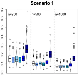
We conduct extensive simulations to evaluate the proposed methods. In all sce-narios, the dimension of the covariate space is 10. Binary treatments A are generated from {−1,1} with equal probability. Three different scenarios are presented, with outcomes generated as follows.
Scenario 1. We simulate the first half of patients from X1, X2 ∼ N(1,1),
X3, . . . , X10 ∼N(0,1) and the second half of patients with X1, . . . , X10 from
logT= exp{0.6∗X1−0.8∗X2+A∗c(X)}+ log.
Here, c(X) = 1 for the first half of patients and c(X) = −1 for the other half, andis generated from an exponential distribution with mean 1. Censoring time Cis generated from Uniform[0,1]. The censoring percentage is around 24%. The optimal decision boundary isd∗(X) = sign(X1+X2−1).
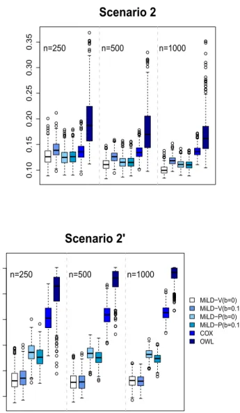
Scenario 2.X1, . . . , X10are generated fromN(0,1). The survival time is the
minimum ofτ= 4 and T, where Tis generated with the hazard rate function
λT(t|X, A) = exp[0.6X1+ 0.8X2−1 +{2X1+ 3(X2+ 1)2−2}A].
Censoring timeC is generated from Uniform[0,5]. The censoring percentage is around 42%. The optimal decision boundary is d∗(X) =−sign{2X1+ 3(X2+
1)2−2}.
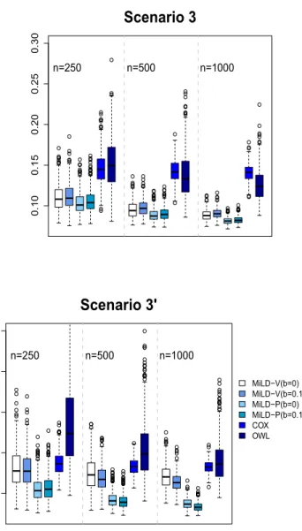
Scenario 3.X1, . . . , X10are generated fromN(0,1). The survival time is the
minimum ofτ= 4 and T, which is generated with
log(T) =X1+X2+ 1 +A(2X13+ 2X2+ 0.5) +N(0,1).
Censoring timeC is generated from
log(C)∼X1+X2+X3+N(0,1).
The censoring percentage is around 51%. The optimal decision boundary is d∗(X) = sign(2X13+ 2X2+ 0.5).
We also consider settings where there is a mismatch between the trial partici-pants and the target population, and we will denote these mismatch scenarios as Scenarios 1’, 2’, and 3’ respectively. In Scenario 1, half of the patients will gain benefits from treatment 1 in both populations. We modify it in Scenario 1’ such that the proportion of patients with d∗(x) = 1 is 1/3 in the trial population, and 1/2 in the target population. In Scenario 2’, we let the covariate distri-bution in the trial data with X1 ∼N(−0.25,1.5) and other covariates
follow-ingN(0,1.5), which are different from the distribution in the target population with all covariates generated fromN(0,1). Eligibility criteria are usually applied for the trial recruitment, and thus trials might selectively enroll patients from the target population. Instead of randomly choosing patients for participation in the trial, patients are selectively enrolled with certain probability, denoted by π(X), into the trial data. In Scenario 3’, the model for the enrollment is logit{π(X)} = −2X3
1 −1, where logit(t) = log{t/(1−t)}. Hence, covariates
predictive of participation in the trial could be predictive of treatment effects, where patients withd∗(x) = 1 are less likely to participate in the trial. Subse-quently, the covariate distributions in trial data and the target population are not the same.
W1(x) andW2(x)≡1 in MiLD, targeted to optimize the value and the allocation
rate to the optimal rule, respectively. We denote them as MiLD-V and MiLD-P. The results might be affected with possible deviations between the target and the trial populations. When we do not have prior information on the target population, we can vary (ν, ρj) to evaluate the resulting changes. As suggested
in Section2.5, we setρj =b Σj F,ν={
j(bˆμj)(Σj+b Σj FIp)(bμˆj)}/2, j=
±1. Here, Σj F is the Frobenius norm of Σj, and bis a constant that reflects
the deviations relative to the covariance matrix norms and the means, in the trial populations. We consider two cases withb= 0 andb= 0.1 for both MiLD-V and MiLD-P.
We compare the proposed methods to the following two approaches.
1. OWL (outcome weighted learning): we find the best linear decision rule by directly targeting maximizing the overall expected outcome (Zhao et al.,
2012).
2. COX: we find the linear decision rule based on a Cox regression model, where interactions betweenX andAare included.
All methods are performed by deriving the best linear treatment rules using trial data. We then calculate the misclassification rate under the estimated rules via Monte Carlo methods. Specifically, a large testing dataset of 10,000 from the target population is generated. Training datasets representing the trial pop-ulation are repeatedly simulated, and each time the rules yielded by various methods are evaluated on this testing set. Different training data sample sizes n = 250,500 and 1000 are considered. We report the average misallocation to non-optimal treatments over 500 replicates. We also report the expected overall survival of the estimated rules using the derived treatment rules by different methods in the supplementary materials.
Fig 1. Misallocation rates in Scenarios 1 and 1’ using trial data with sample sizes varying
from 250 to 1000. The misallocation rate is evaluated by using 500 Monte Carlo repetitions.
5. Data Analysis
Fig 2. Misallocation rates in Scenarios 2 and 2’ using trial data with sample sizes varying
from 250 to 1000. The misallocation rate is evaluated by using 500 Monte Carlo repetitions.
Fig 3. Misallocation rates in Scenarios 3 and 3’ using trial data with sample sizes varying
from 250 to 1000. The misallocation rate is evaluated by using 500 Monte Carlo repetitions.
measured, including Bone alkaline phosphatase (BAP, range 1.9–1761.0 u/L), C-terminal of type 1 collagen (CICP, range 1.4–273.6 ng/mL), N-telopeptides of type 1 collagen (NTx, range 1.4–480.0 nM) and pyridinoline (PYD, range 0.3–15.0 nmol/L). The distribution of bone marker concentrations and serum PSA were skewed with a wide range; therefore, we use log transformation for these variables. All covariates are then standardized for analysis. We intend to find the optimal linear treatment rule that is robust to a potential difference between the trial population and the future population.
We compare the proposed methods with Cox regression and OWL method. Practitioners often directly generalize the results from a clinical trial to the general patient population. However, It is not uncommon that the participants in clinical trials are in general more healthier than the patient population, due to the restrictions on patient eligibility. Hence, in our data analysis, we mimic this phenomenon by changing the distribution of healthier patients in the trial population and the target population. We categorize patients to healthier pa-tients whose serum PSA is below the median level and sicker papa-tients whose serum PSA is above the median level. We employ a cross-validated type anal-ysis. At each run, we partition the whole data set into 5 pieces, where 2 parts of the data are used as training data to estimate the optimal rules, and the remaining part as the validation set for evaluating the estimated rules. Specif-ically, each training data set consists of 2/3 healthier patients and 1/3 sicker patients; on the other hand, each validation set contains 1/3 healthier patients and 2/3 sicker patients. Thus, there is a substantial discrepancy between the training set and the validation set, which represents the trial population and the target population, respectively. The cross-validated values are obtained by averaging the empirical value on all 3 validation subsets. To adjust for censoring when calculating the empirical values, we use inverse probability of censoring weighting techniques, where the empirical value for a treatment decision rule d is calculated by Pn[ ˜Y I{A = d(X)}]/Pn[ ˜I{A = d(X)}], with ˜Y equaling to ΔY /SˆC(Y|A, X). We use a kernel estimator developed in Li et al. (1999) to
obtain ˆSC(t|A, X), which does not require a model assumption. The procedure
is repeated 200 times. The averages and standard errors of these values are re-ported in Table1, where a larger value corresponds to a longer expected survival time. The results show better performances of both MiLD-V and MiLD-P proce-dures compared to other methods. MiLD-V performs the best perhaps because it targets to optimize the value directly.
We then apply the proposed methods to the whole data set. The coefficients in the treatment decision rule recommended by MiLD-V and MiLD-P are presented
Table 1
Mean (s.e.) cross-validated values (days)
COX OWL MiLD-V MiLD-P
b= 0 b= 0.1 b= 0 b= 0.1
749.2 (69.8) 711.1 (71.2) 764.6 (70.2) 765.0 (68.9) 753.5 (69.4) 753.7 (69.4)
Table 2
Coefficients for the estimated linear decision rules by MiLD-V and MiLD-P using the SWOG0421 data
MiLD-V MiLD-P Intercept 0.021 0.037
Age 0.538 0.150 Baseline serum PSA -0.510 -0.734 Bisphosphonate usage (YES = 1) 0.787 1.235 Metastatic disease beyond the bones (YES = 1) -0.301 0.008 Pain (YES = 1) -0.272 0.050 Performance Status (‘2-3’ = 1) 0.515 0.796
BAP 0.382 0.972
CICP -0.023 0.302 NTx 0.137 0.657 PYD -0.339 -0.326
in Table 2. The results yielded by MiLD-V and MiLD-P are close, where 80% of the patients receive the same treatment recommendation. In Figure4(a), we compare the Kaplan–Meier curves for overall survival between two treatment arms. There does not appear to be separation. However, when comparing the group whose treatment assignments were in accordance with the treatments recommended by MiLD-V or MiLD-P with the other group, the Kaplan–Meier survival curves show a clear separation, as shown in Figures4(b) and (c).
6. Discussion
In practice, it is preferable to use interpretable decision rules when communi-cating with clinical practitioners about treatment recommendation. A canonical example is linear decision rule, which is attractive because it can be easily under-stood, and thus can be used to guide future research. Our present work shows that it is possible to identify high-quality linear decision rule that leads to a greater overall benefit, even if the truth may be nonlinear. Furthermore, the proposed method is robust across future populations, taking into account the fact that the study sample may not be representative.
We consider survival time outcomes in this paper. Such endpoints are critical in many settings especially in oncology. However, MiLD can be readily applied for binary or continuous outcomes, provided that we can use existing nonpara-metric methods to obtain preliminary estimates of the decision boundaries. Pop-ular methods for binary outcomes include support vector machine and boosting (Hastie et al., 2009), and for continuous outcomes, we can apply random for-est (Breiman, 2001) and support vector regression (Vapnik et al., 1997). Our current proposal suggests an L2 penalty for handling high-dimensional
Fig 4. Kaplan–Meier survival curves of overall survival in castration-resistant prostate cancer
patients: (a) by treatment received; (b) by accordance between treatment recommended by V and treatment received; (c) by accordance between treatment recommended by MiLD-P and treatment received.
simultaneously, which would eliminate the unimportant variables and further improve the ease of interpretation. Another interesting extension of the current work is to consider settings involving more than two treatments. While it is straightforward to conduct a series of pairwise comparisons, further develop-ment is required to identify the best rule among all treatdevelop-ments. It will also be interesting to investigate extensions to Boolean combination of linear rules, i.e., rules of the form{X1β11+β01≥0} ∩ {X2β21+β02≥0}.
Appendix A: Appendix
max
α,β1,β0
α s.t. inf
X†∼( ˜μ†1,Σ†1)∈U1†
β0+ ˜μ†1β1≥κ(α)
β1Σ†1β1
inf
X†∼( ˜μ†−1,Σ†−1)∈U−1†
−β0−μ˜†1β1≥κ(α)
β1Σ†−1β1,
whereκ(α) =α/(1−α). As shown in Lanckriet et al. (2003),
min
μj:( ˜μ†j−μ†j)Σ†−1j ( ˜μ†j−μ†j)≤ν2
β1μ˜†j=β1μ†j−ν
β1Σ†jβ1,
and maxΣ†:Σ†−Σ†F≤ρβ1Σ†β1 = β1(Σ† +ρIp)β1, where Ip is the identified
matrix. Recall thatUj†={(˜μ†j,Σ†j) : (˜μ†j−μj†)Σ†j(˜μ†j−μ†j)≤ν2, Σ†
j−Σ†j F ≤
ρj}, j = ±1, We have β0+β1μ˜†j = β0+β1μ†j−ν
β1Σ†jβ1, and β1Σ†jβ1 =
β1(Σ†j+ρjIp)β1. We thus further rewrite the optimization problem to
max
α,β1,β0
α s.t. β0+β1μ†1≥κ(α)
β1(Σ†1+ρ1Ip)β1
−β0−β1μ†−1≥κ(α)
β1(Σ†−1+ρ−1Ip)β1.
We will assume thatμ†1=μ†−1; otherwise, the above problem is not identifi-able. We also assume that Σ†j, j=±1 are both positive definite. Sinceκ(α) is a monotone increasing function ofα, we can rewrite our problem as
max
κ κ s.t., β
1μ†−1+κ
β1(Σ†−1+ρ−1Ip)β1≤β0≤β1μ†1−κ
β1(Σ†1+ρ1Ip)β1,
and these inequalities will become equalities at the optimum. We can eliminate the equality constraint by lettingβ1=β10+F u, where u∈Rp−1,β10= (μ†1−
μ†−1)/ μ†1−μ†−1 2
2, and F ∈Rp×(p−1) is an orthogonal matrix whose columns
span the subspace of vectors orthogonal toμ†1−μ†−1. Hence, the optimization problem can be written as in (2). The optimal
β∗0=β∗1μ˜†1−κ∗
β1∗(Σ†1+ρ1Ip)β1∗=β1∗μ˜†−1+κ∗
β1∗(Σ†−1+ρ−1Ip)β∗1,
whereκ∗ is the optimal value ofκwith
κ∗= β1∗(Σ−†1+ρ−1Ip)β∗1+
β1∗(Σ1†+ρ1Ip)β1∗
−1
.
The lower bound on the worst case allocation rateα∗= (κ∗−ν)2/{1 + (κ∗−
ν)2}, andν should not exceedκ∗.
Proof of Theorem 1. We first show that|μˆ†j−μ†j| =Op(r
2γ γ+2
n +n−1/2) and
Σ†j−Σ†j =Op(r
2γ γ+2
n +n−1/2), j=±1, whereW(X) =W1(X) = |fˆ(X)| and
A = supx∈X Ax 2. For the convergence rate in means,
≤ |PnXfˆ(X)I{dˆ(X) =j} − PXfˆ(X)I{dˆ(X) =j}| + |PXfˆ(X)I{d(X) =ˆ j} −PXfm(X)I{d(X) =ˆ j}| + |PXfm(X)I{d(X) =ˆ j} −PXf∗(X)I{d(Xˆ ) =j}| + |PXf∗(X)I{d(Xˆ ) =j} −PXf∗(X)I{d∗(X) =j}| = (I) + (II) + (III) + (IV).
We will use McDiarmid’s inequality to bound (I).
n1
n
k=1
xkfˆ(xk)I{d(xˆ k) =j} −
1 n
n
k=1,k=i
xkf˘i(xk)I{d(x˘ k) =j}
− 1
nx˘if˘i(˘xi)I{d(˘˘xi) =j}
≤1 n
n
k=1
xk{fˆ(xk)−f˘i(xk)}I{d(xˆ k) =j}
+
1 n
n
k=1
xkf˘i(xk)[I{d(xˆ k) =j} −I{d(x˘ k) =j}]
+1 n
(xi−x˘i) ˆf(xi)I{d(xˆ i) =j}+ ˘xi{f(xˆ i)−f˘i(˘xi)}I{d(xˆ i) =j}
+ ˘xif˘i(˘xi)[I{d(xˆ i) =j} −I{d(˘˘xi) =j}]≤Mρ/n,
where Mρ depends onM, CX andρ. The last inequality follows from
Assump-tions1, 5and6.
By McDiarmid’s inequality,
P(|PnXfˆ(X)I{d(X) =ˆ j} −PXfˆ(X)I{d(Xˆ ) =j}| ≥)≤e−2n2/Mρ2.
Then with probability≥1−δ,
|PnXfˆ(X)I{d(X) =ˆ j} −PXfˆ(X)I{d(Xˆ ) =j}| ≤cM
log(1/δ)
n . (7)
For (II), by Cauchy-Schwaz inequality and the boundedness ofX,
|PXfˆ(X)I{d(Xˆ ) =j} −PXfm(X)I{d(Xˆ ) =j}| ≤ P{fˆ(X)−fm(X)}2P(X2)
= Op(rn),
where the last step follows from Assumption4. For (III),
≤ P{fm(X)−f∗(X)}2P(X2)
≤ M f∗−fm 2.
For (IV),
|PXf∗(X)I{d(X) =ˆ j} −PXf∗(X)I{d∗(X) =j}| = |PXf∗(X)I{d∗(X) =j,d(Xˆ )=d∗(X)}|
≤ |PXf∗(X)I{d∗(X) =j}I{0<|f∗(X)| ≤ |f∗(X)−fˆ(X)|}| ≤ |P[Xf∗(X)I{d∗(X) =j}]P{0<|f∗(X)| ≤ |f∗(X)−fˆ(X)|}|
≤ |P[Xf∗(X)I{d∗(X) =j}]P[I{0<|f∗(X)| ≤}I{|f∗(X)−fˆ(X)| ≤} +I{|f∗(X)−f(Xˆ )|> }]|
≤ μ†j
f∗−fˆ 2 2
2 +
γ
,
where f 2 =E{f(x)2}1/2. Choosing the optimal as f∗−fˆ
2
γ+2
2 , we have
that
|PXf∗(X)I{d(Xˆ ) =j} −PXf∗(X)I{d∗(X) =j}| ≤ μ†j f∗−fˆ
2γ γ+2 2 ≤ M r 2γ γ+2
n + f∗−fm
2γ γ+2
2
. (8)
Combining the above results, we obtain that with probability≥1−δ,
|μˆ†j−μ†j| ≤M f∗−fm min(1, 2γ γ+2)
2 +r
min(1,γ2+2γ )
n
+cM
log(1/δ)
n .
Therefore,|μˆ†j−μ†j|isOp( f∗−fm
min(1,2γ γ+2)
2 +r
min(1,2γ γ+2)
n +n−1/2).
We then consider the bound on Σ†j − Σj† , j = ±1. Let Fˆ(X) =
n
i=1fˆ(Xi)I{d(Xˆ i) = j},Fm(X) =
n
i=1fm(Xi)I{d(Xˆ i) = j} andF∗(X) =
n
i=1f∗(Xi)I{d(Xˆ i) =j}. With probability≥1−δ,
Σ†j=
n
i=1
W(Xi)I{d(Xˆ i) =j}
n
i=1W(Xi)I{d(Xˆ i) =j}
2
(Xi−μˆ†j)(Xi−μˆ†j).
Σ†j−Σ†j
≤
(Pn−P)
⎡ ⎣
ˆ f(X)
ˆ F(X)
2
(X−μˆ†j)(X−μˆ†j)I{d(X) =ˆ j}
⎤ ⎦
+ P ⎡ ⎣ ˆ f(X)
ˆ F(X)
2
(X−μˆ†j)(X−μˆ†j)I{d(Xˆ ) =j}
⎤ ⎦
− P f∗(X)
F∗(X)
2
(X−μ†j)(X−μ†j)I{d∗(X) =j}
≤ cδ
log(1/δ) n + P ⎡ ⎣ ˆ f(X)
ˆ F(X)
2
(X−μˆ†j)(X−μˆ†j)I{d(X) =ˆ j}
⎤ ⎦ − P ⎡ ⎣ ˆ f(X)
ˆ F(X)
2
(X−μ†j)(X−μ†j)I{d(X) =ˆ j}
⎤ ⎦ + P ⎡ ⎣ ˆ f(X)
ˆ F(X)
2
(X−μ†j)(X−μ†j)I{d(Xˆ ) =j}
⎤ ⎦ − P ⎡ ⎣ ˆ f(X)
ˆ F(X)
2
(X−μ†j)(X−μ†j)I{d∗(X) =j}
⎤ ⎦ + P ⎛ ⎝ ⎡ ⎣ ˆ f(X) ˆ F(X) 2
− f∗(X) F∗(X)
2⎤
⎦(X−μ†j)(X−μ†j)I{d∗(X) =j}
⎞ ⎠
≤ cδ
log(1/δ)
n + 2
P ⎡ ⎣ ˆ f(X)
ˆ F(X)
2
(X−μ†j)(ˆμj†−μ†j)I{d(X) =ˆ j}
⎤ ⎦ + P ⎡ ⎣ ˆ f(X)
ˆ F(X)
2
{(ˆμ†j−μ†j)(ˆμ†j−μ†j)I{d(Xˆ ) =j}
⎤ ⎦ + P ⎡ ⎣ ˆ f(X)
ˆ F(X)
2
(X−μ†j)(X−μ†j)I{d∗(X) =j,d(X)ˆ =d∗(X)}
⎤ ⎦ + P ⎛ ⎝ ⎡ ⎣ ˆ f(X) ˆ F(X) 2
− fm(X) Fm(X)
2⎤
⎦(X−μ†j)(X−μ†j)I{d∗(X) =j}
⎞ ⎠ + P
fm(X)
Fm(X)
2
− f∗(X) F∗(X)
2
(X−μ†j)(X−μ†j)I{d∗(X) =j}
≤ Op( f∗−fm
min(1,γ2+2γ )
2 +r
min(1,γ2+2γ )
n +n−1/2).
Now we prove Theorem 1’s result. Define
M(u) =
(β10+F u)(Σ†1+ρ1Ip)(β10+F u)
+
and
Mn(u) =
( ˆβ10+ ˆF u)(Σ1†+ρ1Ip)( ˆβ10+ ˆF u)
+
( ˆβ10+F u)(Σ†−1+ρ−1Ip)( ˆβ10+ ˆF u),
where we use the estimated Σ±1,Fˆ and ˆβ10 in M(u). Since u belongs to a
compact set, ˆβ10 → β10,Σj → Σj and ˆF → F, supu|Mn(u)−M(u)| → 0 in
probability. Given that M(u) has a unique maximizer and u is in a compact set, we have supu−u∗≥M(u)< M(u∗). Hence the conditions of Theorem 5.7 of van der Vaart (1998) are satisfied, and it follows that ˆu→u∗ in probability, and subsequently ˆβ1→β1∗ in probability.
We now show the convergence rate of ˆβ1 to β∗1. Given that u → M(u) is
twice differentiable at u∗, we have M(u)−M(u∗)−c u−u∗ 2 for all uin
the neighborhood of u∗ and some c >0, where u∗ is the unique maximizer of
M(u). Since|μˆj−μj|=Op(Op( f∗−fm
min(1,γ2+2γ )
2 +r
min(1,γ2+2γ )
n +n−1/2) and
Σj−Σj =Op( f∗−fm
min(1,γ2+2γ)
2 +r
min(1,γ2+2γ )
n +n−1/2),
|(Mn−M)(u)−(Mn−M)(u∗)|
= |{Mn(u)−Mn(u∗)} − {M(u)−M(u∗)}|
∂Mn(u)
∂u −
∂M(u) ∂u
u=u∗
u−u∗
≈ ( f∗−fm min(1, 2γ γ+2)
2 +r
min(1,γ2+2γ )
n +n−1/2) u−u∗ .
Thus,
E∗ sup
u−u∗<δ|(Mn−M)(u)−(Mn−M)(u
∗)|
( f∗−fm min(1, 2γ γ+2)
2 +r
min(1,γ2+2γ )
n +n−1/2)δ.
Whenδ→φ(δ) =√n( f∗−fm min(1, 2γ γ+2)
2 +r
min(1,γ2+2γ)
n +n−1/2)δ,φ(δ)/δη is
decreasing for anyη∈(1,2). In addition, ˆu→u∗in probability, and ˆumaximize Mn(u). The conditions of Theorem 14.4 in Kosorok (2008) are satisfied with
φ(δ) = √n( f∗ −fm min(1,
2γ γ+2)
2 +r
min(1,γ2+2γ)
n +n−1/2)δ. Hence, u−u∗ =
Op( f∗−fm
min(1,γ2+2γ )
2 +r
min(1,γ2+2γ )
n +n−1/2), and the desired result follows.
Acknowledgments
Supplementary Material
Supplementary Materials for “Robustifying Trial-Derived Optimal Treatment Rules for A Target Population”
(doi:10.1214/19-EJS1540SUPP; .pdf).
References
Audibert, J.-Y., Tsybakov, A. B., et al. “Fast learning rates for plug-in classi-fiers.” The Annals of statistics, 35(2):608–633 (2007).MR2336861
Biau, G. “Analysis of a random forests model.” Journal of Machine Learning Research, 13(Apr):1063–1095 (2012).MR2930634
Breiman, L. “Random forests.” Machine learning, 45(1):5–32 (2001).
MR3874153
Brinkley, J., Tsiatis, A., and Anstrom, K. J. “A generalized estimator of the attributable benefit of an optimal treatment regime.” Biometrics, 66(2):512– 522 (2010).MR2758831
Buchanan, A. L., Hudgens, M. G., Cole, S. R., Mollan, K., Sax, P. E., Daar, E., Adimora, A. A., Eron, J., and Mugavero, M. “Generalizing evidence from randomized trials using inverse probability of sampling weights.” Pharmacy Practice Faculty Publications, Paper 77 (2016).
Cole, S. R. and Stuart, E. A. “Generalizing Evidence From Randomized Clinical Trials to Target Populations The ACTG 320 Trial.” American journal of epidemiology, 172(1):107–115 (2010).
Devroye, L., Gy¨orfi, L., and Lugosi, G. A probabilistic theory of pattern recog-nition, volume 31. Springer Science & Business Media (2013).MR1383093
Goldberg, Y. and Kosorok, M. R. “Q-learning with censored data.” Annals of statistics, 40(1):529 (2012). MR3014316
Greenland, S. “Randomization, statistics, and causal inference.” Epidemiology, 1(6):421–429 (1990).
Hamburg, M. A. and Collins, F. S. “The path to personalized medicine.” New England Journal of Medicine, 363(4):301–304 (2010).
Hastie, T., Tibshirani, R., and Friedman, J. H. The Elements of Statistical Learning. New York: Springer-Verlag New York, Inc., second edition (2009).
MR2722294
Hayes, D. F., Thor, A. D., Dressler, L. G., Weaver, D., Edgerton, S., Cowan, D., Broadwater, G., Goldstein, L. J., Martino, S., Ingle, J. N., et al. “HER2 and response to paclitaxel in node-positive breast cancer.” New England Journal of Medicine, 357(15):1496–1506 (2007).
Hern´an, M. A. and Robins, J. M. “Estimating causal effects from epidemiological data.” Journal of epidemiology and community health, 60(7):578–586 (2006). Huang, X., Ning, J., and Wahed, A. S. “Optimization of individualized dynamic treatment regimes for recurrent diseases.”Statistics in medicine, 33(14):2363– 2378 (2014).MR3256672
Kang, C., Janes, H., and Huang, Y. “Combining biomarkers to optimize patient treatment recommendations.”Biometrics, 70(3):695–707 (2014).MR3261788
Kosorok, M. R. Introduction to empirical processes and semiparametric infer-ence. New York: Springer-Verlag (2008).MR2724368
Lanckriet, G. R., Ghaoui, L. E., Bhattacharyya, C., and Jordan, M. I. “A robust minimax approach to classification.”The Journal of Machine Learning Research, 3:555–582 (2003).MR1991086
Lara, P. N., Ely, B., Quinn, D. I., Mack, P. C., Tangen, C., Gertz, E., Twar-dowski, P. W., Goldkorn, A., Hussain, M., Vogelzang, N. J., et al. “Serum biomarkers of bone metabolism in castration-resistant prostate cancer pa-tients with skeletal metastases: results from SWOG 0421.” JNCI: Journal of the National Cancer Institute, 106(4) (2014).
Li, K.-C., Wang, J.-L., Chen, C.-H., et al. “Dimension reduction for censored regression data.” The Annals of Statistics, 27(1):1–23 (1999).MR1701098
Marshall, A. W. and Olkin, I. “Multivariate chebyshev inequalities.”The Annals of Mathematical Statistics, 31(4):1001–1014 (1960).MR0119234
Orellana, L., Rotnitzky, A., and Robins, J. M. “Dynamic regime marginal structural mean models for estimation of optimal dynamic treatment regimes, part I: main content.”The International Journal of Biostatistics, 6(2) (2010).
MR2602551
Qian, M. and Murphy, S. A. “Performance Guarantees for Individualized Treat-ment Rules.” The Annals of Statistics, 39:1180–1210 (2011).MR2816351
Quinn, D. I., Tangen, C. M., Hussain, M., Lara, P. N., Goldkorn, A., Moin-pour, C. M., Garzotto, M. G., Mack, P. C., Carducci, M. A., Monk, J. P., et al. “Docetaxel and atrasentan versus docetaxel and placebo for men with advanced castration-resistant prostate cancer (SWOG S0421): a randomised phase 3 trial.” The Lancet Oncology, 14(9):893–900 (2013).
Robins, J. M., Hern´an, M. ´A., and Brumback, B. “Marginal structural models and causal inference in epidemiology.” Epidemiology, 11(5):550–560 (2000).
MR1766776
Rubin, D. B. “Bayesian Inference for Causal Effects: The Role of Randomiza-tion.” The Annals of Statistics, 6:34–58 (1978).MR0472152
Tsybakov, A. B. “Optimal aggregation of classifiers in statistical learning.”
Annals of Statistics, 32:135–166 (2004).MR2051002
van der Vaart, A.Asymptotic Statistics. New York: Cambridge University Press (1998).MR1652247
Vapnik, V., Golowich, S. E., and Smola, A. “Support vector method for function approximation, regression estimation, and signal processing.” Advances in neural information processing systems, 281–287 (1997).
Zhang, B., Tsiatis, A. A., Laber, E. B., and Davidian, M. “A robust method for estimating optimal treatment regimes.” Biometrics, 68(4):1010–1018 (2012).
MR3040007
Zhao, Y.-Q., Zeng, D., Laber, E. B., Song, R., Yuan, M., and Kosorok, M. R. “Doubly robust learning for estimating individualized treatment with cen-sored data.” Biometrika, 102(1):151–168 (2015).MR3335102
Indi-vidualized Treatment Rules using Outcome Weighted Learning.” Journal of American Statistical Association, 107:1106–1118 (2012).MR3010898