E
XCEL
S
PREADSHEET
M
ANUAL
to accompany
C
ALCULUS FOR THE
L
IFE
S
CIENCES
G
REENWELL •
R
ITCHEY •
L
IAL
Paula Grafton Young
Salem College
J. Todd Lee
Elon College
Boston San Francisco New York
London Toronto Sydney Tokyo Singapore Madrid Mexico city Munich Paris Cape Town Hong Kong Montreal
All rights reserved. No part of this publication may be reproduced, stored in a retrieval system, or transmitted, in any form or by any means—electronic, mechanical, photocopying, recording, or otherwise—without the prior written permission of the publisher. Produced in the United States of America.
Part I: General Instructions 1 Part II: Detailed Instructions 11
Chapter 1: Functions 13
The Least Squares Line 13
Quadratic Functions 14
Chapter 2: Exponential, Logarithmic, and Trigonometric Functions 16
Exponential Functions 16
Chapter 3: The Derivative 17
Limits 17
Rates of Change 17
Chapter 7: Integration 19
Area and Definite Integrals 19
Chapter 8: Further Techniques and Applications of Integration 20
Numerical Integration 20
Chapter 10: Matrices 22
Solution of Linear Systems 22
Addition and Subtraction of Matrices 25
Multiplication of Matrices 25
Matrix Inverses 26
Chapter 11: Differential Equations 27
Part I:
In this part, we give an overview of the general concepts and tools that involve spreadsheets. The spreadsheet software we use is Microsoft’s Excel 2000 in the MS-Windows 98 environment, but the principles should hold for any current software package.
Spreadsheets
Introduction
One could argue that the advent of spreadsheet and word-processing software ushered in the PC as a primary tool in every workplace. In today’s world, wherever there is a table of data, it is stored in a spreadsheet. Some of the things one can do with data via spreadsheets are:
• Data Arrangement
• Calculation
• Visualization
• Database Management
• Statistical Analysis
• Predictions
• Optimization
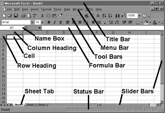
Spreadsheet packages also come with powerful built-in programming languages, making their versatility almost limitless. The best part about spreadsheets is that the initial learning curve is very short! We use Microsoft Excel 2000 for all demonstrations in this manual, but due to the standardization in today’s spreadsheets, one should be able to apply this material to almost any spreadsheet package. Throughout this manual, spreadsheet and PC terminology will be used. In Figure 1, the typical window one sees is displayed with many of the names we use in this manual.
Files
Collections of sheets are stored in files called workbooks. When you open Excel, it starts with a brand new workbook called “Book1.xls”. Figure 1 is very close to what you will see. Notice the title of the workbook in the title bar at the top of the window. If you want to open a previously saved workbook, you can do so through File Æ Open on the menu bar or open it directly by finding the file and double-clicking it.
Each workbook consists of sheets, accessed via the sheet tabs at the bottom of the screen (Figure 1). Each sheet can be either a chart or a worksheet. Charts are any kind of visualization of data, such as scatter plots or bar graphs. Worksheets are the “spreadsheets”, the place where we (and the program) do all of the work.
Cells
Everything begins with the cell. If you can understand exactly what a cell is and what properties it has, the rest should be relatively easy. It is crucial that you understand this section!
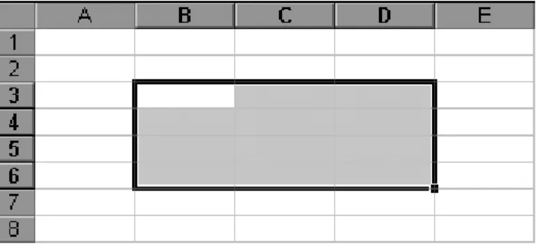
A cell is one of the many rectangles you see on a worksheet. One or more cells are selected when they are surrounded by a bold outline with a fill handle in the lower right hand corner of the outline (we will discuss the purpose of the fill handle later). You can select a single cell by clicking on it or select a rectangular set of them by click-dragging (Figure 2)
Figure 2: The range B3:D6 is selected.
The cell’s primary function is to hold and display “stuff”. The cell has four major attributes, which you must learn:
• Address
• Format
• Content
• Value Cell Address
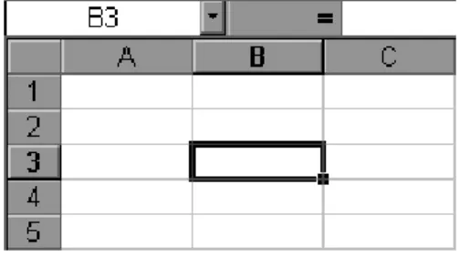
The address of a cell is indicated by the row and column in which it sits. (If you have ever played Battleship®, you know exactly how this works!) The column heading is always one or two letters (ranging from A to IV) and the row heading is always a number (from 1 to
65536). A cell’s address consists of the column letter(s) and the row number. For example, if a cell sits in column B and row 3, then its address is B3 (Figure 3). Note: The address of the selected cell is given in the name box.
Figure 3: The address of the selected cell is B3
When a rectangular range of cells is selected, the address of the range is given by the address of the upper left cell and the lower right cell, separated by a colon. In Figure 2 the upper left cell of the selected range is B3 and the lower right cell is D6, thus the range is denoted by
B3:D6. Note: When a range of cells forms a single column or row, the two end cells are used to denote the range.
Cell Format
A cell can contain many things, like numbers and text, but how the cell displays those things can vary greatly. Suppose you type into every cell of a range (say B1:B5) the number 0.75. Without any formatting, the cells all display 0.75. By right-clicking a cell, you bring up a plethora of options, including Format Cells… (like most everything else, this can also be obtained through the menu bar). The first tab you get in the Format Cells pop-up window is Number (Figure 4). Here is where you can format the cell to display its value as anything from dates to currency. You can even dictate how many decimal places the cell will display (which can cause Excel to round the displayed value but not the actual value). In Figure 5 you can see some of the possibilities, where all the cells contain the same value 0.75.
Cell Content
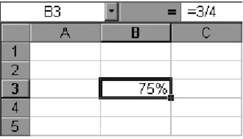
The content of a cell is whatever you type into it, which is usually a number, text, or a formula. The content of the cell is not necessarily what the cell displays! In other words, you may type a formula into a cell and press Enter, then what the cell displays is the value of the formula, while the content of the cell is the formula. Whenever you select a cell, the content of the cell is shown in the formula bar. For example suppose you select a cell, type the formula
=3/4, and press Enter. If you formatted the cell as a percentage, then the cell will display the value 75%. Now reselect cell, look in the formula bar and you should see the formula =3/4
(Figure 6).
Figure 6: Cell B3 displays 75%, has a value of 0.75, and contains the formula =3/4.
This is what makes spreadsheets so powerful. You will be able to enter formulas into cells that use values from other cells. In turn, these other cells may contain formulas themselves!
There is something very important to remember when using longer, more complicated formulas in Excel. Excel does not correctly obey the standard order of operations! Recall from basic algebra that and ( , because an exponent applies only to whatever is to its immediate left. Unfortunately, Excel is programmed to apply negation (the negative sign)
before applying exponents, whether parentheses are present or not. So the formula =–A1^2 will return the value of –A1 squared, not the negative of A1 squared. Therefore, when using Excel, you should adopt the convention of enclosing the base and the exponent in parentheses. Table 1 shows the result of three different formulas. If you wish to calculate , then you should use the formula shown in the last column of the table.
9 32 =−
− −3)2 =9
2
3
−
A2 =A2^2 =-A2^2 =-(A2^2) 3 9 9 -9
Table 1.
Cell Value
Every cell has a numeric value, even an empty one (which has a default value of 0). If you type a number into a cell, then that will also be the cell’s value. If you type a numeric formula into a cell, then that cell’s value will be the outcome of the formula. When the cell contains text or has a formula that returns text, then the value of that cell will default to 0. Remember, the value of a cell, what the cell displays, and the cell’s content are three different things. As seen in the example illustrated in Figure 6, the value of the cell is a 0.75, while the cell’s content is the formula =3/4 and the cell’s display is 75%.
Formulas
As seen earlier, you can type formulas into a cell. All formulas start with an “=”. A formula can have numbers, algebraic operations, functions, and addresses for cells and ranges. Notice that we do not have variables! Any time we want to use a value from another cell in a formula, we can use the cell’s address instead. Let us consider an example.
Suppose you wanted to store in cell D2 the average of three numbers that you have stored in cells B1, B2 and B3. This can be done with a formula. In cell D2, type =(B1+B2+B3)/3
and press Enter. The cell D2 displays the average. If you reselect cell D2, the formula bar will display the formula that the cell contains, while the cell displays its value (Figure 7).
Figure 7: Average of cells via a simple formula.
For many common calculations (such as averaging) there are built-in functions. To view a list of these functions, click on a cell and type “=”. The name box changes and becomes a drop-down list of functions you have used recently, but right now the most interesting choice is More Functions… (Figure 8). Through this choice, you can explore and use a whole host of functions; it is certainly worth your while to check this out! Another way of obtaining a function is through the menu bar Insert Æ Function. You can also type in functions directly if you know the correct spelling and appropriate arguments. In Figure 9, the function =AVERAGE(B1:B3)
gives the same result as seen in Figure 7.
Figure 8: Average of cells via a simple formula. Figure 9: Average of cells via a simple formula.
Copy, Paste, and Fill
Anyone who has used a PC is probably quite familiar with cut, copy, and paste. When copying cells, if the cell’s content is anything other than a formula, the contents are identically transcribed. However, when the content of a copied cell is a function, then the addresses within the function are adjusted by the relative distance from the copied cell to the pasted cell.
As an example, consider Figure 10 where you have a table of values of which you want the average of each column. Type in the appropriate formula for averaging the first column, copy that cell and paste into the cell under the next column (Figure 11). Notice how the address range
A1:A3 is shifted by exactly one column value to B1:B3. This is precisely the relative change from the copied cell (A4) to the pasted cell (B4). If you pasted from the cell A4 to the cell C9, the relative change would be two to the left and five down, thus the pasted formula would be
=AVERAGE(C6:C8).
Figure 10: The first average function is typed in. Figure 11: The next average is copied from the first.
Figure 12: The fill handle is grabbed and dragged. Figure 13: All of the averages are correctly filled in.
Coming back to our example, there is a much quicker way of copying one cell to multiple cells. The technique is called filling, and with most things, there are several ways of accomplishing it. As noted earlier, every highlighted cell has a fill handle in the lower right-hand corner. If you hold-click this handle (grab) and drag in any direction, an automatic copy/paste is performed on all covered cells. In Figure 12 the handle on cell B4 is shown grabbed and dragged across cells C4 and D4. When the mouse is released, the average function is pasted into the both
C4 and D4 with the appropriate adjustment to the address ranges within the function (Figure 13). There may be times when you will copy/paste a cell and you want one or more parts of the address ranges in the function’s arguments to not change. The trick is to use a $ in front of every part of the addresses you want to freeze. For instance, suppose you are filling from a cell with the formula =A1+B3-C7. If you do not want the column of the address A1 to change, you would instead use the formula =$A1+B3-C7. If you do not want the row address of B3 to change, you would use the formula =A1+B$3-C7. If you do not want the address C7 to change at all, you would use the formula =A1+B3-$C$7. When an address is completely frozen, e.g. $C$7, this is called an absolute reference. When no part of the cell reference is frozen, e.g. C7, this is called a relative reference. When part of a cell reference is frozen, e.g. $C7 or C$7, this is called a mixed reference.
Charts
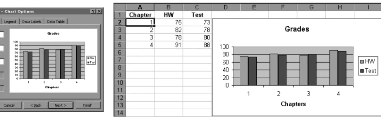
A picture is worth a thousand words. Spreadsheets are loaded with graphical tools for displaying sets of data. The best part is how easy it is to create a chart of data. Consider the data in Figure 14 of homework and test grades over the first four chapters of a class. Select the data to be visualized (range B1:C5) and engage the chart wizard via the tool bar or the menu under Insert. As seen in Figure 15, the first screen of the chart wizard gives many choices of possible charts, including bar charts, pie charts, and scatter plots. The default choice is the standard grouped bar graph.
Figure 14: These are class grades to be visualized.
Figure 15: There are a host of choices in charts.
Figure 16: The chart wizards gives lots
of control over the chart. Figure 17: The chart can be added to the data spreadsheet or placed on a separate sheet.
As you move through the wizard, you are given a vast number of choices to fine tune and annotate your graph (Figure 16). The last choice you need to make is whether or not the chart will be displayed on the data spreadsheet or given a sheet of its own (Figure 17).
After the chart is created, changes can be made by simply right-clicking the part of the chart in which you are interested. For example, if you want to change the format of the title, right-click it and select Format Chart Title from the resulting menu. You can make major changes to the whole chart by right-clicking in the white area of the chart, outside of any parts. The resulting menu allows you to change everything from chart type to gridlines. Later in this manual you will see how by right-clicking the data graphics, one can even include trendlines!
Conclusion
Once you become comfortable with the spreadsheet environment, you should experiment with all the available charts, formulas, and built-in abilities. The possibilities for effectively and efficiently using Excel, or any other spreadsheet program, are practically endless. If you are using Microsoft Word or Microsoft PowerPoint, all tables and charts from Excel can be copied and pasted into a Word document or PowerPoint presentation so that you can create attractive papers and presentations. You can even import data from other programs and databases, as well as from the World Wide Web. Even though this manual only demonstrates how to use Excel for problems that arise in finite mathematics and in applied calculus, Excel also has applicability to other courses, including statistics, accounting, economics, biology, chemistry, and physics, just to name a few.
You may also find spreadsheets useful for keeping track of your college credits, personal finances, even as an address book for e-mail and mailing addresses and phone numbers. You are limited only by your imagination and patience.
Part II:
Part II contains detailed steps and instructions for using Microsoft’s Excel 2000 to complete many examples from Calculus for the Life Sciences. Most of the instructions provided can be applied to other spreadsheet programs.
Part II is organized by chapter; since not all chapters require detailed explanations of spreadsheet use, some chapters are not covered in this manual. Section titles form the textbook are indicated in italics. References are made to specific examples and exercises from the corresponding sections of each chapter, so you should have your textbook nearby as you read through these instructions.
Chapter 1: Functions
The Least Squares Line
Finding the Least Squares Regression Line.
To complete the example in this section, begin by entering the lists of data points into columns A and B. We can now use the functions SLOPE, INTERCEPT, and CORREL to find
m, b, and r, respectively. Type the following into the indicated cells: Cell Contents
E1 =SLOPE(B2:B10,A2:A10)
E3 =INTERCEPT(B2:B10,A2:A10)
E5 =CORREL(B2:B10,A2:A10)
When using the SLOPE and INTERCEPT functions, the list containing the y-values must be first, as shown above. The final result should resemble Table 1.
Year Death Rate Slope = -0.55667 10 84.4
20 71.2 y-intercept = 90.22222 30 80.5
40 73.4 r = -0.94956 50 60.3
60 52.1 70 56.2 80 46.5 90 36.9
Table 1.
Displaying Data and The Regression Line on the Same Graph.
Begin by entering the lists of data points and creating an XY (Scatter) chart in the spreadsheet. (See Part I of this manual for additional assistance with creating charts.) Right-click on any data point in the chart and select Add Trendline. Select the first type, Linear, then click the Options tab. Check the boxes in front of “Display equation on chart” and “Display R-squared value on chart”. Click OK and the least squares line and the resulting value of r2 are displayed. You may need to click and drag the text box containing the equation and r2 value to move it to a more convenient position within the chart. The final result should resemble Figure 1.
y = -0.5567x + 90.222
R2 = 0.9017
0 20 40 60 80 100
0 50 100
Death Rate Linear (Death Rate)
Figure 1.
It is important to remember that this method gives you r2, which is the square of the correlation coefficient. To find the value of r, you must take the square root of this value, or use the
CORREL function as described previously.
Quadratic Functions
Quadratic Regression.
In Example 6 of this section of your text, a quadratic function is fit to a set of data representing lead emissions. The quadratic regression feature of Excel can be used to complete this example. There are two ways to do this, but the easiest by far is to begin by creating a scatter plot of the data set. Begin by entering appropriate column headings for the year and the lead emissions. (See Table 2.)
Year (Since 1990) Lead Emissions (in 1000 tons) 2 3808 3 3911 4 4043 5 3924 6 3910 Table 2.
Enter the data, using the numbers 2 through 6 to represent the years 1992 through 1996. Highlight the data set, including column headings, and select Insert, then Chart. Choose the XY (Scatter). Click Finish to see the chart. Right-click on any data point in the chart and select Add trendline. Select the Polynomial type, and make sure that “2” is selected as the “order” since we wish to fit a second degree polynomial to the data. Click the Options tab and select “Display equation on chart.” Click OK. The quadratic model, and its equation, will be displayed on the chart. The result should appear similar to Figure 2. (You may wish to drag and move the equation box to keep it from interfering with the rest of your chart.)
y = -34.643x
2+ 298.84x + 3347.4
3750 3800 3850 3900 3950 4000 4050 4100
0 2 4 6 8
Figure 2.
This polynomial trendline feature of Excel can be used to fit up to a sixth degree polynomial model to a set of data. To do so, simply change the “order” to the degree of the polynomial you wish to fit.
Power Regression.
In Exercise 7(b) from the review exercises of your textbook, you are asked to use power regression to fit an appropriate model to a set of data. Following the same procedures as outlined on the next page for Exponential Regression, use the Power type when adding a trendline.
Chapter 2: Exponential, Logarithmic, and
Trigonometric Functions
Exponential Functions
Exponential Regression.
Example 7(b) of this section of the text asks us to find an exponential function that models the given climate data. For simplicity, subtract 1990 from each year, so that 1990 becomes year “0”, 2000 becomes year “10”, and so on. After entering appropriate column headings, enter the years and the corresponding carbon dioxide levels in adjacent columns. Follow the instructions given above for creating a scatter plot and adding a trendline. For the trendline type, select Exponential.
Chapter 3 The Derivative
Limits
Creating Limit Tables.
As indicated in the discussion following Example 1, limits of functions can be estimated by observing appropriate values of a function in a table. To use Excel to estimate the limit in this example, begin by choosing appropriate column headings and entering, in column A, a list of x -values that surround x = 2. (See Table 1.) Enter the following contents into cell B2 and drag to fill the rest of column B:
Cell Contents
B2 =(A2^2+4)/(A2-2)
x (x^2+4)/(x-2) 1.9 -76.1 1.99 -796.01 1.999 -7996.001 1.9999 -79996.0001 2.0001 80004.0001 2.001 8004.001 2.01 804.01 2.1 84.1 Table 1. Rates of Change
Estimating Instantaneous Rates of Change.
To generate the table in Figure 22 from this section of your text, choose appropriate column headings, like those in Table 2, for the value of h, the value of f(x+h), the value of f(x), and the value of the difference quotient. Enter the following values into the appropriate cells: Cell Contents
A2 .1
B2 =369*0.93^(2+A2)*(2+A2)^0.36
C2 =369*0.93^2*2^0.36
D2 =(B2-C2)/A2
h f(x+h) f(x) Inst. Rate of Change 0.1 413.846707 409.602937 42.43770666 0.01 410.041368 409.602937 43.84309816 0.001 409.646924 409.602937 43.98729544 0.0001 409.607337 409.602937 44.00175289 0.00001 409.603377 409.602937 44.00319903 0.000001 409.602981 409.602937 44.00334359
Table 2.
It should be clear from observing the last column of Table 2 that, as h approaches 0, the instantaneous rate of change of f(x) is approximately 44.003 when x = 2.
Chapter 7 Integration
Area and Definite Integrals
Summation.
To use Excel to complete Example 1 from this section of your text, type in appropriate column headings, similar to those in Table 1. In column A, type in the numbers 1 through 4, to indicate the number of the rectangle. In column B, type in the x-values representing the midpoints of the bases of the rectangles. Enter the following contents into the indicated cells:
Cell Contents
C2 =2*B2 (evaluate f(x) at B2)
F1 1 (the value of ∆x)
Drag and fill the rest of column C. Since we now wish to sum the values , we can do this with a SUM command. In cell C6, type =SUM(C2:C5)*$F$1. The result should look similar to Table 1.
x x
f( i)∆
i xi f(xi) Delta-x 1 1 0.5 1 2 1.5 3 3 2.5 5 4 3.5 7 Sum: 16
Chapter 8: Further Techniques and
Applications of Integration
Numerical Integration
The Trapezoidal Rule.
As indicated in the discussion after Example 1 in your text, the trapezoidal rule can be done quickly with Excel. Begin by creating column headings for the i, xi, and f(xi). To complete
Example 1, fill column A with the integer values 0 through 4. Next, enter the following contents into the indicated cells:
Cell Contents
B2 =$F$1+A2*$F$2
C2 =SQRT(B2^2+1) (evaluate the function)
F1 0 (the left endpoint for the definite integral)
F2 0.5 (the value of ∆x)
Notice the absolute cell references for F1 and F2, since you will want the same left endpoint and
∆x throughout. Highlight cells B2 and C2, then drag to fill columns B and C. Finally, to apply the trapezoidal rule, in cell F3, type =F2*(0.5*C2+SUM(C3:C5)+0.5*C6). The result should appear similar to Table 2 below.
i xi f(xi) Left endpoint 0 0 0 1 Delta-x 0.5 1 0.5 1.118034 Approximation 2.976529
2 1 1.414214 3 1.5 1.802776 4 2 2.236068
Table 4.
Simpson’s Rule.
To complete Example 2 via Simpson’s rule on Excel, set up a table exactly like the one you set up for the trapezoidal rule. In cell F3, which will contain the Simpson’s rule approximation for the integral, type =(F2/3)*(C2+4*C3+2*C4+4*C5+C6). The result should appear similar to Table 3 below.
i xi f(xi) Left endpoint 0 0 0 1 Delta-x 0.5 1 0.5 1.118034 Approximation 2.957956
2 1 1.414214 3 1.5 1.802776 4 2 2.236068
Chapter 10: Matrices
Solution of Linear Systems
Row Operations.
As indicated in your text, a clever use of the Copy and Paste Special commands can minimize the arithmetic required by the Gauss-Jordan Method for solving systems of linear equations. Begin by setting up the matrix, with appropriate row and column headings, in the cell range A1:E4, as shown in Table 1.
x y z Constant R1 1 -1 5 -6
R2 3 3 -1 10
R3 1 3 2 5
Table 6.
Highlight the entire matrix, including the row and column headings, select Copy from the Edit
menu, and click on cell A6. Select Paste from the Edit menu to paste the entire matrix. Since the first row operation we are asked to perform is –3R1 +R2→R2, highlight the entire second row of
the copied matrix and type in the following: Cell Contents
B8 =-3*B2:E2+B3:E3
Do not press Enter! Instead, press Ctrl-Shift-Enter (all three keys simultaneously). This will
cause each of the cells in our copied R2 to be updated with the values resulting from the row
operation. To complete the next row operation, –R1 +R3→R3, highlight the entire third row of
the copied matrix and type in the following, pressing Ctrl-Shift-Enter when finished: Cell Contents
B9 =-B2:E2+B4:E4
The new matrix, with the updated rows, should look like Table 2.
x y z Constant R1 1 -1 5 -6
R2 0 6 -16 28
R3 0 4 -3 11
Now, highlight the entire new matrix, and select Copy from the Edit menu. Click on cell
A11, and this time, select Paste Special from the edit menu. In the window that pops up, select
Values and click OK. This will copy only the values, not the formulas, from the previous matrix operations. To perform the next row operation from this example in your text, highlight the first row of the third matrix, type =B8:E8+6*B7:E7, and press Ctrl-Shift-Enter to update the new row. Notice that we are now creating our formulas from the second matrix, the one that was updated. To finish with the third matrix, select the third row, type =2*B8:E8-3*B9:E9 and press Ctrl-Shift-Enter. This matrix should now look like Table 3.
x y z Constant R1 6 0 14 -8
R2 0 6 -16 28
R3 0 0 -23 23
Table 8.
Continue by copying and using the Paste Special command to create the fourth matrix, and make sure you create the formulas by referencing the previously completed matrix, until the process is complete.
The Solver.
Excel’s built-in Solver can find solutions to many different types of systems of equations. Among the types of systems Solver can solve are systems of linear equations with unique solutions. The Solver should be located in the Tools menu of Excel. If it is not, you will need to locate your original installation disk, select Add-Ins from the Tools menu, and install the Solver program.
You should take care to set up a worksheet that contains as much helpful information as possible, including headings for rows, columns, and even individual cells, so that you can keep track of what all the entries represent. To complete Example 2 from your text using Solver, we can set up a worksheet similar to that in Table 4, with the following formulas in the indicated cells:
Cell Contents
B3 =B1+D1+5*F1
B4 =3*B1+3*D1-F1
B5 =B1+3*D1+2*F1
x= y= z=
x-y+5z=-6 0 = -6 3x+3y-z=10 0 = 10
x+3y+2z=5 0 = 5
From the Tools menu, select Solver. Type in the address of the cell containing the first formula, in this case, cell B3, as the “Target Cell”, then check “Value of” and type in the value of the constant for the first equation, which is -6 in this example. The cells we wish to change are the cells next to the labels for x, y, and z, so type B1,D1,F1 into the box below “By Changing Cells”. Our constraints here are the equations themselves, and we have already typed these in. Select Add, and type in the name of the cell containing the first formula. Select “=” from the drop-down menu, then type in the name of the cell containing the constant from the first equation. If your worksheet is set up like Table 4, then the Add window should appear as in Figure 1. If so, click Add.
Figure 1.
Now, we need to add the second equation as a constraint, so type in B4 as the “Cell Reference”, select “=” from the drop-down menu, and enter D4 as the “Constraint”. We need to add one more equation, so click Add again and repeat this process for the third equation. When it is entered, click OK. This will return you to the Solver window, which should now look like Figure 2.
Figure 2.
Click Solve. The program will now adjust the values of the variables until all constraints are satisfied, if possible. The top row of the worksheet should now contain the solution to the system of equations, x = 1, y = 2, and z = -1.
The Solver cannot solve systems of equations that have no solution, nor can it solve systems with infinitely many solutions. If you try to use it to solve one of these types of systems, a new window will appear letting you know that Solver was unable to complete the problem.
Addition and Subtraction of Matrices
Example 7 of this section of your text can be completed with Excel by first entering the matrices, C and K, then using a Ctrl-Shift-Enter trick as we did with the matrix row operations. This technique is highly useful if there are large matrices that need to be added or subtracted.
To complete Example 7, enter the matrices C and K into a worksheet, in a manner similar to Table 5. Then, highlight a block of empty cells that is the same size as the answer should be. In this case, you need to highlight a block of cells that is two rows by three columns. While the empty block is highlighted, type =A2:C3-E2:G3. This indicates that the first matrix is located in the cell range A2:C3 and we wish to subtract from it the second matrix, whish is located in the range E2:G3. Press Ctrl-Shift-Enter and the empty block will be filled with the resulting matrix. (See Table 5.)
C K
22 25 38 5 10 8 31 34 35 11 14 15
C-K
17 15 30 20 20 20
Table 10. Multiplication of Matrices
The MMULT function in Excel can be used to multiply matrices. To complete Example 4 of this section of your text, enter the two matrices to be multiplied, A and B, and highlight a block of empty cells that is the same size as AB should be. In this case, we need to highlight a block of cells that is three rows by three columns. Type =MMULT(A2:B4,D2:F3) and press
Ctrl-Shift-Enter to see the resulting product. Similarly, the product BA can be calculated by highlighting a set of empty cells that is 2 rows by 2 columns, typing
A B
1 -3 1 0 -1 7 2 3 1 4 -2 5
AB BA
-8 -3 -13 3 -8 13 2 1 2 13 13 5 22
Table 11. Matrix Inverses
Once a square matrix has been entered into a worksheet, its inverse can be calculated with the MINVERSE function. To complete Example 1 from this section of your text, enter matrix A, then highlight a set of empty cells that is the same size as the inverse should be, which is in this case 3 rows by 3 columns. Type =MINVERSE(A2:C4) and press Ctrl-Shift-Enter to calculate the inverse. (See Table 7.)
A A-inverse
1 0 1 0 0 0.333333 2 -2 -1 -0.5 -0.5 0.5 3 0 0 1 0 -0.33333
Table 12.
A Note About Round-off Errors and Matrix Inverses.
Occasionally, when performing calculations involving matrix inverses, one or more entries in the resulting matrix may look like 1E-10, or something similar. Keep in mind that this represents 1 times 10 to the -10th power, or 0.0000000001. A result like this in a problem that originally contained no numbers of this form is due to round-off error during Excel’s calculations. Usually, it is safe to treat any similar results as “0.”
Chapter 11: Differential Equations
Euler’s Method
Example 1 of this section of the text can be completed using Excel. Set up the sheet with columns for the independent variable x, the approximate solution variable y, the actual solution
f(x), and the error y-f(x). You also need a single cell containing the step h. Table 1 shows the set-up with the proper initial values in the range A1:E4.
x y f(x) y-f(x) h
0.0 1.5 1.5 0.0 0.1
Table 13.
The contents of all the cells in the second row are numbers except for D2, which contains the difference formula =B2-C2. The third row will be all formulas, as seen in the following:
Cell Contents
A3 =A2+$E$2
B3 =B2+$E$2*(A2-2*A2*B2)
C3 =0.5+Exp(-(A2^2))
D3 =B3-C3
Notice the absolute references for cell E2, as you want to use the same step size h throughout the calculations. Now select the range A3:D3 and fill down nine rows. Your results should be identical to Table 2.
x y f(x) y-f(x) h
0 1.5 1.5 0 0.1 0.1 1.5 1.49005 0.00995 0.2 1.48 1.460789 0.019211
0.3 1.4408 1.413931 0.026869 0.4 1.384352 1.352144 0.032208 0.5 1.313604 1.278801 0.034803 0.6 1.232243 1.197676 0.034567 0.7 1.144374 1.112626 0.031748 0.8 1.054162 1.027292 0.026869 0.9 0.965496 0.944858 0.020638 1 0.881707 0.867879 0.013827