Scientic Computing 2013 Computer Classes: Worksheet 11: 1D FEM and boundary conditions

Scientic Computing 2013

Computer Classes: Worksheet 11:

1D FEM and boundary conditions

Oleg Batrashev

November 14, 2013

This material partially reiterates the material given on the lecture (see the slides) and then presents dierent types of boundary conditions and how to apply them in FEM.

1 Finite Element Method

The main idea of FEM is to replace the space of all functionsV with much smaller subspace a space of piecewise linear functions v ∈Vh (see Figure 1). Provided the pointsxi, where linearity

breaks, it is possible to express all such functions using basis functions ϕi ('hat' functions)

v(x) =Xηiϕi(x)

Variational formulation Another idea is to rewrite a dierential equation using weak formula-tion, which has almost the same solution as the original problem. Particularly, Poisson's equation in 1D

−u00(x) =f(x), x∈[0,1]

may be rewritten using variational formulation ˆ 1

0

u00vdx=

ˆ 1 0

f vdx, ∀v∈V

v(x)

ϕ2

0 1

1

where test functions v are usually taken to be the same as basis functionsϕi above.

It is not convenient to have second-order derivative u00, so it is possible to replace it with the rst-order derivatives using integration by parts

− ˆ 1

0

u00vdx=−u0v

1 0+

ˆ 1 0

u0v0dx (1)

1.1 Dirichlet boundary condition

If we a given Dirichlet boundary conditionu(0) =u(1) = 0, then Equation 1 loosesu0v (v is from the same space asu, thusv(0) =v(1) = 0). TheM×M stiness matrixA= (aij)and right-hand

sidebare calculated with aij =

ˆ 1 0

ϕ0_iϕ0_jdx, bi=

ˆ 1 0

f ϕidx, i, j= 1, . . . , M

Task 1

Given xi and f(x) write a script that solves the Poisson equation with Dirichlet boundary

condition using FEM. Hints:

ˆ the initialization may look like N = 10

xs = linspace (0 ,1 ,N +1) M = len (xs )-2

A = np. asmatrix (np. zeros ((M,M ))) def f(x):

return -.4+x ˆ ´1

0 ϕiϕjdxmay be calculated directly usinghvalues (see lecture slides) ˆ ´1

0 f ϕicould be calculated using scipy.integrate.quad()

phi = np. vectorize ( get_phi (i)) xa = xs[i -1]

xb = xs[i +1]

r = integrate . quad ( lambda x:f(x)* phi (x),xa ,xb )[0] ˆ where get_phi(j) returnsϕjfunction

def get_phi (j): def _phi (x):

if x <= xs[j -1] or x >= xs[j +1]: return 0.

elif x <= xs[j]:

return (x-xs[j -1])/( xs[j]-xs[j -1]) else :

return (xs[j+1] -x )/( xs[j+1] - xs[j]) return _phi

-0.002 0 0.002 0.004 0.006 0.008 0.01 0.012 0.014 0.016 0.018

0 0.2 0.4 0.6 0.8 1

(a) with uniformh

-0.002 0 0.002 0.004 0.006 0.008 0.01 0.012 0.014 0.016 0.018

0 0.2 0.4 0.6 0.8 1

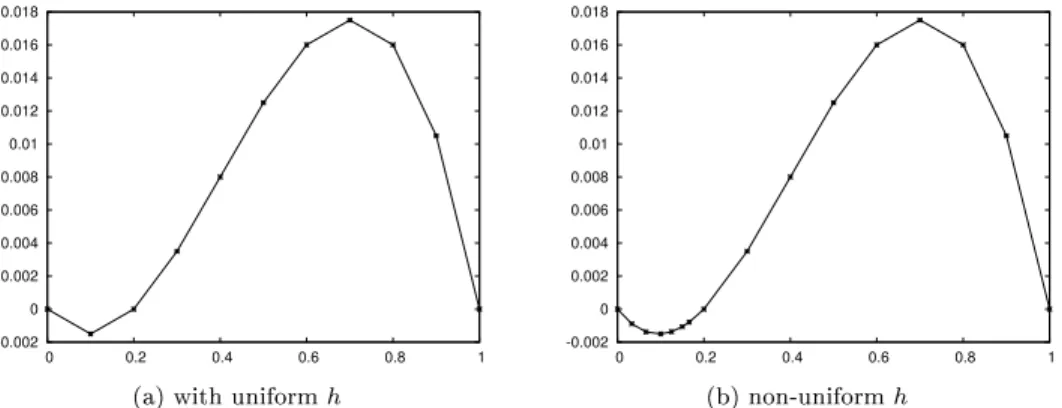
(b) non-uniformh Figure 2: Solution for Poisson's equation with f(x) = 0.4−x

Example. The following output shows the matrix A, the right-hand side b and the solution u (ys) for the uniformh= 0.1andf(x) = 0.4−x:

Listing 1: k= 5andu0(0) = 0.2

xs = [ 0. 0.1 0.2 0.3 0.4 0.5 0.6 0.7 0.8 0.9 1. ]

A

[[ 20. -10. 0. 0. 0. 0. 0. 0. 0.]

[ -10. 20. -10. 0. 0. 0. 0. 0. 0.]

[ 0. -10. 20. -10. 0. 0. 0. 0. 0.]

[ 0. 0. -10. 20. -10. 0. 0. 0. 0.]

[ 0. 0. 0. -10. 20. -10. 0. 0. 0.]

[ 0. 0. 0. 0. -10. 20. -10. 0. 0.]

[ 0. 0. 0. 0. 0. -10. 20. -10. 0.]

[ 0. 0. 0. 0. 0. 0. -10. 20. -10.]

[ 0. 0. 0. 0. 0. 0. 0. -10. 20.]]

b = [ -0.03 -0.02 -0.01 0. 0.01 0.02 0.03 0.04 0.05]

ys = [ 0.00000000 e +00 -1.500000e -03 -5.51271630e -18 3.500000 e -03 8.00000000 e -03 1.25000000 e -02 1.60000000 e -02 1.75000000 e -02 1.60000000 e -02 1.05000000 e -02 0.00000000 e +00]

Figures 2a and 2b show solutions correspondingly for the uniform h = 0.1 and the following

non-uniform case

xs = np. array ([ 0., .033 , 0.066 , .1, .125 , .15 , .166 , .2, .3, .4, .5, .6, .7, .8, .9, 1.])

2 Other boundary conditions

FEM is well applicapable with dierent boundary conditions and complex geometries. Here we try the former and the example of complex geometry can be presented with 2D FEM.

2.1 Mixed boundary condition

Mixed boundary condition means that part of the boundaryΓ(e.g left in our case) has Neumann

boundary condition (u0(x) =c)while other part (right) has Dirichlet boundary condition (u(x) =d). Particularly, in our case we try

u0(0) =c, u(1) = 0

First observation is that the test function ϕ0 is now non-zero because left edge is not xed, so

we have to introduce new unknown u0. The test function is however only half of a typical test

function.

Another observation comes from Equation 1 whereu0v6= 0withx= 0. This adds−u0_{(0)v(0) =}

−c·1to the right-hand sideb0.

Task 2

Write a script that givenxi and f(x) calculates ui using mixed boundary condition (left

Neumann and right Dirichlet). Hints:

ˆ matrixA and RHS vectorbnow have one more row (rst one), look carefully through all the indices and expressions in the code;

ˆ A0,0is however only half of other diagonal values (becauseϕ0function has twice smaller non-zero domain);

ˆ b0 must be updated with−c.

Example. Withf(x) =−1, uniform h= 0.1andu0(0) =c=−0.5

A

[[ 10. -10. 0. 0. 0. 0. 0. 0. 0. 0.]

[ -10. 20. -10. 0. 0. 0. 0. 0. 0. 0.]

[ 0. -10. 20. -10. 0. 0. 0. 0. 0. 0.]

[ 0. 0. -10. 20. -10. 0. 0. 0. 0. 0.]

[ 0. 0. 0. -10. 20. -10. 0. 0. 0. 0.]

[ 0. 0. 0. 0. -10. 20. -10. 0. 0. 0.]

[ 0. 0. 0. 0. 0. -10. 20. -10. 0. 0.]

[ 0. 0. 0. 0. 0. 0. -10. 20. -10. 0.]

[ 0. 0. 0. 0. 0. 0. 0. -10. 20. -10.]

[ 0. 0. 0. 0. 0. 0. 0. 0. -10. 20.]]

b = [ 0.45 -0.1 -0.1 -0.1 -0.1 -0.1 -0.1 -0.1 -0.1 -0.1 ]

ys = [ 1.20736754 e -16 -4.50000000e -02 -8.00000e -02 -1.050000e -01 -1.20000000e -01 -1.25000000e -01 -1.200000e -01 -1.050000e -01 -8.00000000e -02 -4.50000000e -02 0.00000000 e +00]

Notice, that if you try Neumann BC on both sides you will probably get singular matrixA. This is because there are heat ows given at both sides and heat generation/consumption on domain

[0,1]but no anchor temperature, so the heat equation either gives indenite temperature growth

or has no meaningful solution.

2.2 Robin boundary condition

-0.14 -0.12 -0.1 -0.08 -0.06 -0.04 -0.02 0 0.02

0 0.2 0.4 0.6 0.8 1

Figure 3: Solution for Poisson's equation withf(x) =−1and mixed BC

This condition may be used when there is external temperatureuDand diusion on the boundary

at rate k. The temperature at the boundary tries to achieveuD unless the diusion is bad. Here

we try Robin boundary condition on the left sidex= 0.

The matrix is almost the same as with Mixed boundary condition. From Equation 1 we get kϕ0(0)ϕ0(0) =kmust be added toA0,0andkuDϕ0(0) =kuD tob0.

Task 3

Write a script that givenxi and f(x) calculates ui using Robin boundary condition (left

Robin and right Dirichlet). Hints:

ˆ generation of matrixAis the same is with Mixed boundary condition, except diagonal value in the rst row must be updated

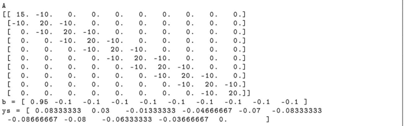
Example. Withf(x) =−1, Robin condition on the left boundaryu0(0) =k(u(0)−uD), k= 5,

uD= 0.2and Dirichlet on the right boundaryu(1) = 0 we get the following

A

[[ 15. -10. 0. 0. 0. 0. 0. 0. 0. 0.]

[ -10. 20. -10. 0. 0. 0. 0. 0. 0. 0.]

[ 0. -10. 20. -10. 0. 0. 0. 0. 0. 0.]

[ 0. 0. -10. 20. -10. 0. 0. 0. 0. 0.]

[ 0. 0. 0. -10. 20. -10. 0. 0. 0. 0.]

[ 0. 0. 0. 0. -10. 20. -10. 0. 0. 0.]

[ 0. 0. 0. 0. 0. -10. 20. -10. 0. 0.]

[ 0. 0. 0. 0. 0. 0. -10. 20. -10. 0.]

[ 0. 0. 0. 0. 0. 0. 0. -10. 20. -10.]

[ 0. 0. 0. 0. 0. 0. 0. 0. -10. 20.]]

b = [ 0.95 -0.1 -0.1 -0.1 -0.1 -0.1 -0.1 -0.1 -0.1 -0.1 ]

ys = [ 0.08333333 0.03 -0.01333333 -0.04666667 -0.07 -0.08333333

-0.08666667 -0.08 -0.06333333 -0.03666667 0. ]

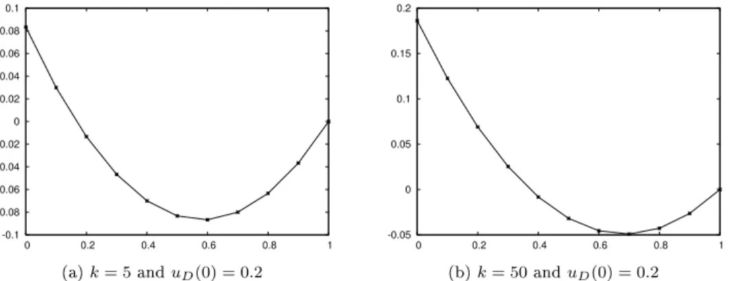
Figure 4 shows corresponding examples with dierent k values. Notice, that value on the boundary converges to the external valueuD as the coecientk increases.

-0.1 -0.08 -0.06 -0.04 -0.02 0 0.02 0.04 0.06 0.08 0.1

0 0.2 0.4 0.6 0.8 1

(a)k= 5anduD(0) = 0.2

-0.05 0 0.05 0.1 0.15 0.2

0 0.2 0.4 0.6 0.8 1

(b)k= 50anduD(0) = 0.2