Risk Appetite and Commodity Returns
Erkko Etula
Harvard University
[email protected]
February 2009
AbstractThis paper shows that the risk appetite of leveraged …nancial institu-tions such as security broker-dealers forecasts commodity returns at quar-terly horizons. The result holds robustly both in-sample and out-of-sample and is particularly strong for energy commodities: the single variable is able to forecast up to 34% of the variation in quarterly crude oil returns. The pattern emerged shortly after the launch of commodity futures contracts and is consistent with a model in which the economic role of broker-dealers is to provide insurance to producers and end-users of commodities. I es-timate cross-sectional prices of risk using an arbitrage-free asset pricing approach and show that broker-dealer risk appetite forecasts commodity returns through its association with market-wide risk premia. Additional predictions of the model for the market risk premium, market volatility, and speculative activity also receive support in the data.
I am grateful to my advisers Jeremy Stein, John Campbell, Ken Rogo¤, and Andrei Shleifer, and to Tobias Adrian, Emmanuel Farhi, Robin Greenwood, Ravi Jagannathan, Hyun Song Shin and Erik Sta¤ord for their comments, support and advice. I also thank seminar participants at the Federal Reserve Bank of New York. All errors are my own.
1. Introduction
The last three decades witnessed impressive growth of leveraged …nancial institu-tions. This trend is displayed in Figure 1.1, which also shows the stark divergence of the growth of U.S. broker-dealer …nancial assets from the growth of household …nancial assets in the late 1970s. While the plot is intriguing in its own right, the economic signi…cance of the growth pattern is further ampli…ed by the procycli-cality of broker-dealer …nancial leverage: Adrian and Shin (2008a) demonstrate that broker-dealer risk appetite ‡uctuates sharply with funding conditions. When liquidity is high, broker-dealer assets expand and leverage is adjusted upward. Conversely, when liquidity is tight, broker-dealer assets contract and leverage must be reduced. Combining the increased importance of the broker-dealer sec-tor with the evidence of aggressive balance sheet management, it seems plausible to conjecture that ‡uctuations in broker-dealer risk appetite are also re‡ected in asset prices.
0.1 1 10
52 56 60 64 68 72 76 80 84 88 92 96 00 04 08
Broker-Dealer Total Financial Assets as a Fraction of Household Total Financial Assets (%, log scale)
Figure 1.1: Broker-dealer total …nancial assets as a share of household total …nan-cial assets, Q1/1952-Q2/2008.
This paper investigates the impact of broker-dealer risk appetite on commodity prices. The paper shows that dealer risk appetite, as proxied by broker-dealer asset growth, has forecasting power for quarterly commodity returns across a cross-section of energy, metal, and agricultural commodities. The result holds robustly both in-sample and out-of-sample and is particularly strong for energy commodities: the single variable is able to forecast up to 34% of the variation in quarterly crude oil returns. The pattern emerged shortly after the launch of commodity futures contracts and is consistent with a model in which the economic role of broker-dealers is to provide insurance to producers and end-users of com-modities. In equilibrium, expected commodity returns re‡ect broker-dealer risk appetite through their association with commodity risk premia.
Figure 1.2 illustrates the emergence of return forecastability for crude oil by plotting the R2 obtained from rolling regressions of crude oil returns on lagged
broker-dealer asset growth. The power of the return forecasts jumps sharply ap-proximately two years after the crude oil futures contract begins trading in the NYMEX and the CME in 1983. This change in the market structure (denoted by the red mark on the time axis) brought transparency into energy pricing and facil-itated the matching of producers and end-users of commodities with speculators willing to supply insurance against ‡uctuations in commodity prices.
To show how the power of the uncovered predictive relationship relates to the size of the dealer sector, Figure 1.2 also reproduces the graph of broker-dealer asset share from Figure 1.1. It may not be surprising that the predictive power of lagged broker-dealer risk appetite has increased over time along with the size of the broker-dealer sector — but what is quite striking, the two variables have also grown at the same rate as indicated by the parallel trend lines. This …nding lends support to the stability of the forecast relationship over time.
The theoretical section of the paper builds on existing literature on commod-ity pricing to argue that the impact of broker-dealer risk appetite on expected
0.1 1 10 52 56 60 64 68 72 76 80 84 88 92 96 00 04 08 0.01 0.1 1 Broker-Dealer Asset Share %,
log scale (left)
R-Squared, 18-Year Rolling Window Ending, log scale (right)
Figure 1.2: Predictive power of lagged broker-dealer asset growth in rolling crude oil return regressions, Q1/1952-Q2/2008. Crude oil futures launched in March 1983.
commodity returns stems from the importance of broker-dealers as “insurance brokers”(speculators) in commodity futures markets. Commodity futures are vi-tal for producers and end-users of commodities (hedgers) because they are the principal means to unload spot commodity price risk. This risk is often termed "non-marketable" because the trading of many spot commodities involves signi…-cant transaction costs or informational asymmetries, which discourage speculators from engaging in spot commodity transactions in the marketplace. These trans-action costs and informational asymmetries are alleviated in the futures market where the hedgers’ demand for insurance is marketed through futures contracts that require no investment outlays. The insurance premia are determined by the risk appetite of speculators who o¤er to bear the price risk. To the extent that hedgers’demand for insurance is independent of the ‡uctuations in speculator risk appetite, changes in speculator risk appetite should in equilibrium be re‡ected in
expected commodity returns.1
The link between broker-dealer risk appetite and expected commodity returns is rationalized in a simple pricing model where broker-dealers maximize expected return on equity subject to a value-at-risk constraint and have a role in providing insurance to producers and end-users of commodities. In equilibrium, expected commodity returns are determined by their loading on systematic marketable risk but also on systematic non-marketable risk whose price ‡uctuates with broker-dealer risk appetite.
The model predicts that broker-dealer risk appetite should be a signi…cant de-terminant of expected returns for those commodities that load particularly heavily on systematic non-marketable (spot commodity) risk. The analysis shows that some energy commodities such as crude oil and its derivatives heating oil and unleaded gasoline have a large positive loading on systematic spot commodity risk, which makes them particularly sensitive to changes in broker-dealer risk ap-petite: high broker-dealer risk appetite forecasts low expected returns on energy commodities as speculators lower their required risk premia. The converse holds for some agricultural commodities such as wheat and cocoa, which have a signi…-cantnegative loading on systematic spot commodity risk. For these commodities, high broker-dealer risk appetite forecasts high expected returns as the risk premia required by speculators decrease. The model is also consistent with other quanti-tative and qualiquanti-tative features of the data, including market risk premia, market volatility, and speculative activity in commodity futures markets.
The paper concludes with cross-sectional asset pricing tests, which con…rm the signi…cance of broker-dealer asset growth for the pricing of systematic spot commodity risk. The results also suggest that the innovations to broker-dealer risk appetite constitute a signi…cant source of systematic risk for the cross-section
1Grossman and Miller (1988) emphasize that hedgers also have a strong preference for
imme-diacy in hedging transactions. This further increases their vulnerability to shifts in speculator risk appetite.
of commodity returns. Overall, the cross-sectional evidence lends strong support to the view that the uncovered forecastability of commodity returns is a re‡ection of systematic changes in risk premia.
1.1. Related Literature
The risk appetite channel analyzed in this paper originates in Adrian and Shin (2008a,b,c) who demonstrate that the active management of …nancial interme-diary balance sheets generates procyclical leverage, which has consequences for investor risk appetite. The authors exhibit evidence that the adjustment of bal-ance sheets forecasts changes in aggregate market volatility, particularly the price of risk of volatility, at weekly horizons. The impact of procyclical leverage on as-set prices is further explored in Adrian, Etula and Shin (2008) who show that the growth of U.S. …nancial intermediary balance sheets has systematic implications for the cross-section of currency returns. The view that balance sheet constraints in‡uence risk premia is also supported by the 2007-2008 …nancial market turmoil, which shows how a sudden drying up of …nancial intermediary liquidity may have signi…cant systematic consequences.
The literature on time-varying expected commodity returns can be divided roughly into two groups of theories. The …rst group uses the CAPM to argue that the expected return on commodity holdings re‡ects their value as a hedge against market ‡uctuations. Early studies include Black (1976) and Breeden (1980) who explain the variation in futures prices by systematic risk that stems from changes in economic state variables. Tests of these models …nd scant evidence in the data, as show by Jagannathan (1985) and a number of other studies. More recently, Bessembinder and Chan (1992) …nd that the same variables that forecast market returns — e.g. dividend yield, interest rate, and credit spread — also forecast commodity returns. This suggests that time-varying risk premia in commodities could be driven by macro-economic forces that determine asset allocation. Gorton
and Rouwenhorst (2006) attribute a lesser role to the hedging value of commodities and argue that commodity futures as an asset class provide a return pro…le that is comparable to that of equities.
The second group of theories argues that the expected return of holding com-modities is driven largely by commodity-speci…c factors. Most relevant for the present paper are the studies that …nd additional forecastability of commodity futures risk premia and returns using the net positions of hedgers in the futures market, which is known as hedging pressure. The idea of hedging pressure dates back to Keynes (1930) and Hicks (1939) whose theory of normal backwardation argues that producers short futures to hedge their initially long positions in the underlying spot. Models that allow both hedging pressure and systematic risk to a¤ect futures prices include Stoll (1979) and Hirschleifer (1988, 1989). Empirical evidence for the combined role of commodity-speci…c hedging pressure and sys-tematic market risk include Carter, Rausser and Schmidt (1992), Bessembinder (1992), and de Roon, Nijman and Veld (2000).
The current paper contributes to the …rst group of theories by demonstrating that for a set of commodities a signi…cant portion of the time-variation in expected returns can be attributed to time-variation in U.S. broker-dealer risk appetite. The paper’s argument for why broker-dealer risk appetite matters for expected commodity returns builds on the second group of theories: broker-dealers have an important role in providing insurance to producers and end-users of commodities who wish to hedge their positions in spot commodities. This channel is also supported by the evidence of Erb and Harvey (2006) who show that such insurance provision earns positive expected excess returns. In sum, the current paper argues that expected commodity returns re‡ect changes in broker-dealer risk appetite through their systematic association with insurance risk premia.
The theoretical framework builds on Danielsson, Shin and Zigrand (2008) where investor risk appetite shifts endogenously with balance sheet constraints
that ‡uctuate with market outcomes, generating endogenous risk. The balance sheet constraints are imposed by a contracting setting of Adrian and Shin (2008c), which yields a value-at-risk rule. The model has similarities with the large behav-ioral …nance literature on noise trader risk (e.g. DeLong, Shleifer, Summers and Waldmann, 1990; Barberis, Shleifer and Vishny, 1998; Hong and Stein, 1999), lim-ited arbitrage (e.g. Shleifer and Vishny, 1997), and market making (e.g. Grossman and Miller, 1988; Kyle, 1985). However, the distinguishing feature of the present framework is its ability to generate stochastic volatility even though the underly-ing fundamental risks remain constant. It is also free of restrictive assumptions on the behavior of noise traders.
The outline of the paper is as follows. To …x ideas, Section 2 develops a simple framework, which introduces broker-dealer balance sheet constraints in an equilibrium pricing model for commodities. The model shows that if broker-dealers play an important role in providing insurance to producers and end-users of physical commodities, then ‡uctuations in broker-dealer risk appetite should be re‡ected in expected commodity returns through their association with risk premia. Section 3 con…rms the predictions of the model in the data by showing that broker-dealer risk appetite forecasts returns on commodities that have the heaviest loadings on systematic spot commodity risk. Section 4 tests additional predictions of the model and incorporates evidence from the commodity futures market. Section 5 implements a cross-sectional asset pricing model with time-varying prices of risk and …nds that balance sheet constraints are signi…cant to the pricing of the cross-section of commodity returns. Section 6 concludes.
2. Theoretical Framework
As discussed above, there is an extensive literature2that relates futures risk premia to two components: systematic marketable risk and commodity-speci…c hedging pressure. The latter arises from risks that agents cannot or do not want to trade because of market frictions such as transaction costs or informational asymmetries. Following this literature, consider an economy with marketable assets A, futures
F, and non-marketable securities N. Denote byrt+1i the excess return on security
i. The non-marketable securities may serve as the underlying value of the futures contracts and can also coincide with some of the assets. While the returns on non-marketable securitiesrN
t+1do not enter the market portfolio, they do in‡uence
portfolio choice.
Suppose there are two types of agents in the economy: risk-neutral broker-dealers and risk averse investors. The portfolio of agentj consists of positions in assets !jA;t, futures !jF;t, and non-marketable securities qtj:
rt+1j =!jA0rAt+1+!Fj0rt+1F +qj0rFt+1:
All positions are expressed as a fraction of the agent’s …nancial wealth. 2.1. Risk-Neutral Broker-Dealers
Security brokers and dealers (bd) are leveraged …nancial institutions that …nance long positions in risky securities (dollar value S1) with short positions in other
risky securities (dollar value S2). Their cash holdings (c) earn the safe rate of
return. A stylized broker-dealer balance sheet can be depicted as: Assets Liabilities
S1
c
e S2
2For example, Stoll (1979), Hirshleifer (1988, 1989), Carter et al. (1983), Bessembinder
wheree is the market value of equity.
Following Danielsson, Shin and Zigrand (2008), suppose broker-dealers maxi-mize expected return on equity subject to a value-at-risk constraint:
max
!A;t;!F;t
Et rt+1bd s:t: V aRt et:
That is, pro…t-maximizing broker-dealers leverage up to the maximum level per-mitted by their balance sheet constraints. Thus, under pro…t maximization, the value-at-risk constraint binds with equality. IfV aRis some multiple of portfolio volatility
q
V art rt+1bd , the constraint becomesV art rt+1bd = et 2
.
Suppose for simplicity that broker-dealers do not have non-marketable securi-ties. It follows that the return on broker-dealer equity is given by:
rt+1bd =!bdA;t0rt+1A +!bdF;t0rt+1F :
The Lagrangian is:
Lt=Et rt+1bd t V art rt+1bd
e 2
: (2.1)
De…nert+1 = rt+1A ; rt+1F
0
, !bdt = !bdA;t; !bdF;t 0, and write the FOC:
!bdt = 1
2 t[V art(rt+1)]
1
Et(rt+1); (2.2)
where!bd
t is the broker-dealer’s optimal portfolio choice.
Note that equation (2:2) is identical to the standard mean-variance choice but with the risk-aversion parameter replaced by t, the Lagrange multiplier
as-sociated with the balance sheet constraint. In other words, broker-dealers are risk-neutral but behave as if they were risk-averse with the risk aversion ‡uc-tuating with market conditions. As the balance sheet constraint binds harder, the shadow price t increases, and leverage must be reduced. The inverse of the Lagrange multiplier, 1
t, measures broker-dealer risk appetite. 3
2.2. Risk-Averse Investors
Suppose the rest of the investors are risk-averse (ra). They trade o¤ mean against variance in the portfolio return, which depends on the returns on assets, futures, and non-marketable securities:
rt+1ra =!raA;t0rt+1A +!F;tra0rFt+1+qtra0rNt+1:
Agentra chooses positions in the marketable securities to solve:
max
!ra t
Et rrat+1 V art rt+1ra ;
which yields the FOC:
!rat = 1 2 [V art(rt+1)] 1 Et(rt+1) [V art(rt+1)] 1Covt rt+1; rt+1N q ra t : (2.3)
Note that the optimal porfolio choices of broker-dealers and risk-averse in-vestors are linked by:
!bdt = t !rat + [V art(rt+1)] 1Covt rt+1; rNt+1 q ra t : (2.4) 2.3. Market Portfolio
Denote byst the share of broker-dealer assets in the economy:
st = Wbd t Wra t +Wtbd :
Since futures contracts are in zero net supply, market clearing implies:
!Mt = ! M A;t 0 = (1 st)!raA;t+st!bdA;t 0 : (2.5) by: t= 2e t q Et(rt+1)0[V art(rt+1)] 1Et(rt+1):
If the market portfolio is e¢ cient in the sense that it satis…es the FOCs(2:2)and
(2:3)for t, , qt, and st, one obtains:
Et(rt+1) = Mt Covt rt+1; rt+1M +Covt rt+1; rNt+1 qtM ; (2.6) where 1 M t = 1 st + st t (2.7) is the aggregate risk appetite and
qtM = (1 st)qtra (2.8)
is the vector of aggregate non-marketable positions on the economy. Note that the aggregates in (2:7) and (2:8) are linear combinations of the two investor groups’ respective variables.
2.4. Equilibrium Returns
Let it =
Covt(rti+1;rMt+1)
V art(rMt+1)
denote security i’s beta with the portfolio of marketable assets and rewrite the expression (2:6) for equilibrium returns as:
Et(rt+1) = tEt rMt+1 + Covt rt+1; rt+1N q M t tCovt rMt+1; r N t+1 q M t M t = tEt rMt+1 + Covt rt+1; rt+1N M tCovt rMt+1; r N M t+1 M t : (2.9)
The second line de…nes:
rt+1N M rt+1N qMt ;
which is interpreted as the excess return on the aggregate production-weighted portfolio of non-marketable securities. If non-marketable securities consist pri-marly of physical commodities, thenrN M
t+1 is the excess return on the world
Further, denote the coe¢ cient of Mt in(2:9)by:
t Covt rt+1; rN Mt+1 tCovt rt+1M ; r N M
t+1 ; (2.10)
which contains the loadings of individual assets on aggregate non-marketable risk in excess of their loadings on aggregate marketable risk. It follows that (2:9)can be expressed concisely as:
Et(rt+1) | {z } Security Risk Premium = t Et rt+1M | {z } Price of Marketable Risk + t |{z}Mt Price of Non-Marketable Risk : (2.11)
The …rst term in(2:11)captures the non-diversi…able risk that stems from ‡uc-tuations in the value of aggregate marketable securities. The price of marketable risk is Et rMt+1 . The second term captures the non-diversi…able risk that stems
from ‡uctuations in the value of aggregate non-marketable securities, which is not already captured by systematic marketable risk. The price of non-marketable risk is M
t and it varies over time with the willingness of broker-dealers to provide
insurance against non-marketable risks — i.e. it varies with broker-dealers’risk appetite as given by(2:7). Note that (2:11) prices both futures and assets.
3. Empirical Implementation
The model outlined in Section 2 implies that risk premia for all futures contracts and spot commodities are determined by two systematic risk components: one that stems from aggregate marketable risk and another that stems from aggregate non-marketable risk. Replacing expectations by realizations in (2:11), assuming constant conditional variances and covariances, and adding a constant on the right hand side yields:
rit+1 = i+ ir M
t+1+ i Mt + i
withE it+1 = 0 and E it+1rt+1M =E it+1 Mt = 0 for all i. Equation(2:7)tells one that the risk premium M
t is proportional to
h st
t 1
i 1
and has the following three properties: First, the risk premium increases as the broker-dealer balance sheet constraints tighten, which increases t and forces a
decrease in leverage. Second, if broker-dealer leverage is procyclical as suggested by the above theoretical model and the empirical evidence of Adrian and Shin (2008a), then broker-dealer assets ‡uctuate in near lock-step with their leverage, which implies that broker-dealer asset growth is a good proxy for broker-dealer risk appetite, 1
t. The empirical tests that follow normalize broker-dealer asset growth
by household asset growth to obtain a proxy for
t 1 . This captures the idea
that it is the deviations of broker-dealer implied risk appetite from household risk tolerance that drive time-varying risk premia. Third, ‡uctuations in broker-dealer risk appetite matter economically only if the share st of broker-dealer assets in
the economy is high enough.
Based on the above properties of M
t , one may conclude that a good proxy
might be the negative of broker-dealer asset growth in excess of household asset growth. The model also suggests that one may bene…t from interacting this proxy with the share of broker-dealer assets, st, to account for any time variation in the
power of the forecasting relationship (recall Fig. 1.2). The interaction is likely to be of particular importance in longer samples.
3.1. Data
The empirical exercises that follow investigate the impact of lagged broker-dealer asset growth on the excess returns of spot commodities and commodity futures. The data on aggregate balance sheets is obtained from the Federal Reserve, which publishes the …gures quarterly as part of the Flow of Funds Accounts. The analysis includes 14 individual commodities and two investable commodity indexes. The individual commodities are selected based on their respective world production
quantities and liquidity of futures contracts.
The price data on spot commodities, commodity futures and commodity in-dexes are obtained from Compustat. The excess returns are generated by sub-tracting the 3-Month Treasury Bill rate from the quarterly gross returns. The data on equity returns, bond returns, and technical indicators used as controls in the regressions are provided by Global Financial Data. The data on the S&P 500 implied volatility index (VIX) and the credit default swap index (CDX) are from Bloomberg.
The paper also employs quantity data on the positions of market participants in futures exchanges. These variables are obtained from the Commitment of Traders reports, which are published weekly by the Commodity Futures Trading Commission. The CFTC requires that large traders in futures exchanges report whether they take a position for hedging (‘commercial’) or for speculative (‘non-commercial’) purposes. To register as a hedger, one must hold a cash position in the underlying. Thus, the hedgers in commodity futures markets consist primarily of producers and end-users of physical commodities: producers (such as farmers) have long positions in the underlying commodity and wish to short the futures contract in order to hedge against spot price ‡uctuations; conversely, end-users (such as ‡our mills) have a future need for the physical commodity and want to long the futures contract in order to lock in the purchase price today. Speculators consist of broker-dealers, hedge funds, and other market participants who hold the futures for other purposes. See Bessembinder (1992) for further discussion of the distinction between commercial and non-commercial traders.
The baseline regressions cover the time period Q3/1990-Q4/2008, which was selected based on the availability of data. Year 2008 is excluded because the key assumption of the model fails to hold in most quarters of the year: the use of broker-dealer asset growth as a proxy for broker-dealer risk appetite 1
t relies on
that is, increases in broker-dealer assets are matched by increases in leverage to keepV aR=Equityconstant. As the …nancial crisis expanded in 2008, a signi…cant part of broker-dealer asset growth was …nanced by equity4. For instance, the
…rst quarter of 2008 witnessed substantial growth in broker-dealer assets while leverage decreased signi…cantly, suggesting that broker-dealer asset growth was not a good proxy for broker-dealer risk appetite. A decrease in risk appetite in Q1/2008 would correctly predict the run-up in oil prices in Q2/2008, which the asset growth proxy fails to capture. Unfortunately, it is hard to …nd reliable aggregate data on broker-dealer leverage. This is a topic for future work.
3.2. In-Sample Regressions
The panels of Table 1 implement the baseline OLS speci…cation of equation(3:1)
for the futures and spot returns of 14 individual energy, metal, and agricultural commodities. Table 1A regresses the quarterly futures excess returns on the S&P 500 excess return and lagged broker-dealer asset growth in excess of household asset growth (henceforth, broker-dealer asset growth). Since the futures contracts are “pure bets”in the sense that they require no investment outlays, their excess returns are given by the percentage price change, pt+1=pt 1. The regressions
consider the returns on the front-month contracts, which are usually the most liquid ones. The results show that broker-dealer asset growth is a signi…cant predictor of expected returns for crude oil, its derivatives heating oil and unleaded gasoline as well as for silver, copper, wheat and cocoa. Note, however, that the sign of the coe¢ cient for most agricultural commodities is positive rather than negative — this feature is consistent with the predictions of the model and will be discussed below. The economic power of the regressions is the strongest for the three energy commodities crude oil, heating oil and unleaded gasoline, for which
4As the crisis escalated, it is possible that the usual stigma associated with equity decreased,
making it a more desirable form of …nancing for broker-dealers. Thus, the …nancing decisions in 2008 …nd some support in the pecking order theory of Myers and Majluf (1984).
the adjusted R2 is over 20%.
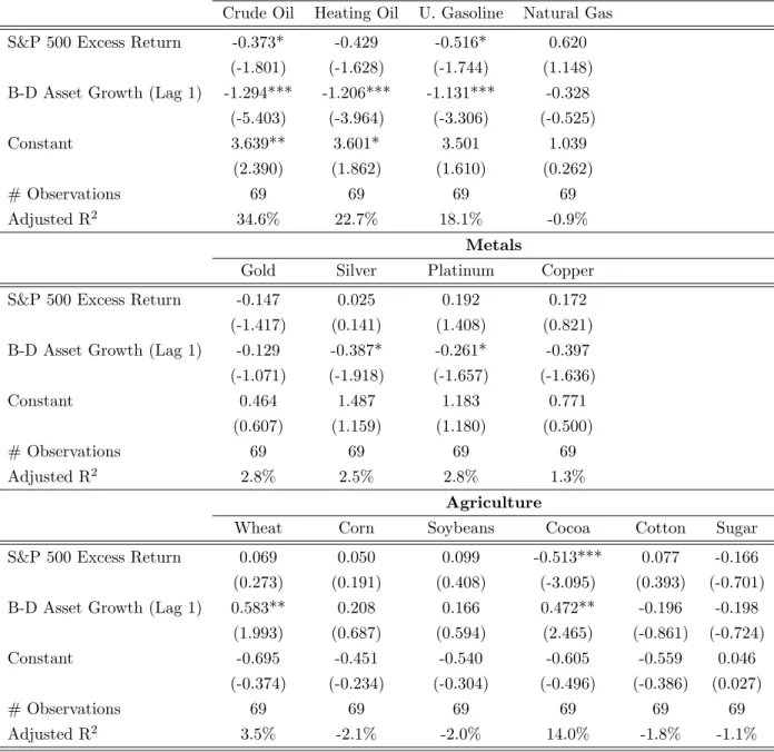
Table 1B conducts the same regressions for excess spot returns. Consistent with the predictions of the model, the results are nearly identical. An additional set of regressions for the futures basis (price of future minus price of spot) as the dependent variable con…rms that broker-dealer risk appetite has no predictive power for the front-month slope of the futures curve at this frequency.
Finally, Table 1C runs the baseline regression for the excess returns on the S&P Goldman Sachs Commodity Index (spot and futures) and the Dow Jones Commodity Index (futures), which are readily accessible to investors. The results show that broker-dealer asset growth is a highly signi…cant predictor of excess returns on all indexes. The table also includes the regression for the Dow Jones Corporate Bond index to show that broker-dealer asset growth has no predictive power for excess bond returns.
While the regressions of Table 1 include the contemporaneous market excess return as an additional predictor variable, one should note that this control has no material impact on the signi…cance of lagged broker-dealer asset growth or the power of the regressions. It is included merely to adhere to the theoretical speci…cation in equation (3:1). The qualitative results also remain una¤ected if broker-dealer asset growth is interacted with the share of broker-dealer assets st.
3.3. Estimated vs. Model-Predicted Loadings
To see how the coe¢ cient estimates of Tables 1A-1C compare with the predictions of the pricing model(2:11), compute the theoretical loadings on M
t of individual
commodity futures, spot returns, and indexes using:
i =Cov rt+1i ; r N M t+1 iCov r M t+1; r N M t+1 ; (3.2)
which is just a stationary version of (2:10). Recall that the weights of the non-marketable portfolio are given by the vector of aggregate non-non-marketable positions
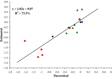
y = 1.02x + 0.07 R2 = 73.3% -1.8 -1.6 -1.4 -1.2 -1.0 -0.8 -0.6 -0.4 -0.2 0.0 0.2 0.4 0.6 0.8 -1.8 -1.6 -1.4 -1.2 -1 -0.8 -0.6 -0.4 -0.2 0 0.2 0.4 0.6 0.8 Theoretical Estimated
Figure 3.1: Commodity futures and futures indexes: Estimated vs. model-predicted coe¢ cients of broker-dealer asset growth for energy (squares), metal (circles) and agricultural (triangles) commodities, plus three indexes (diamonds).
the non-marketable portfolio by the excess return on the GSCI Spot index, which weights commodities by their respective world production quantities.
Since M
t is inversely proportional to broker-dealer asset growth, one must
compare the estimated coe¢ cients of broker-dealer asset growth from Tables 1A-1C with i’s computed by (3:2). Figure 3.1 displays the results for the futures
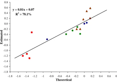
contracts and Figure 3.2 draws the same comparison for the spot commodities. The scatter plots lend substantial support to the model: for both futures and spot commodities, the empirical coe¢ cient estimates line up cleanly with the model-predicted coe¢ cients. For futures, the slope of the relationship is remarkable 1.02 and for the spot commodities the slope is also nearly unity at 0.81. The R2’s of both regressions are well above 70%. The only outlier is natural gas whose estimated coe¢ cient is somewhat less negative than the model-predicted value (see the bottom-left corner of the plots).
under-y = 0.81x + 0.07 R2 = 78.1% -1.8 -1.6 -1.4 -1.2 -1.0 -0.8 -0.6 -0.4 -0.2 0.0 0.2 0.4 0.6 0.8 -1.8 -1.6 -1.4 -1.2 -1 -0.8 -0.6 -0.4 -0.2 0 0.2 0.4 0.6 0.8 Theoretical Estimated
Figure 3.2: Spot commodities and indexes: Estimated vs. model-predicted co-e¢ cients of broker-dealer asset growth for energy (squares), metal (circles) and agricultural (triangles) commodities, plus three indexes (diamonds).
standing why one observes such vast di¤erences in the signi…cance and the fore-cast power of broker-dealer asset growth across commodities. They con…rm the prediction of the model that ‡uctuations in broker-dealer risk appetite should have the greatest impact on the risk premia of those commodities that covary the most with the aggregate non-marketable portfolio; that is, on the commodities that load heavily on the price of systematic non-marketable risk, which ‡uctuates strongly with broker-dealer risk appetite.
3.4. In-Sample Robustness Checks
The remainder of the section will investigate the robustness of the forecasting relationships uncovered in the panels of Table 1. In the interest of space, the analysis will be limited to crude oil and the GSCI index.
The panels of Table 2 display the quarterly in-sample regressions of crude oil excess return (panel A) and GSCI excess return (panel B) on lagged broker-dealer
asset growth and a set of controls. Column (i) shows that the lagged growth of broker-dealer …nancial assets is an important predictor of commodity returns on both statistical and economic grounds: the variable is signicant at 1% level and can alone forecasts nearly 34% of the in-sample variation in the excess crude oil returns and 13% of the GSCI futures returns over the next quarter. Column (ii) demonstrates that the results are not a¤ected by the inclusion of an autoregressive term.
Columns (iii)-(viii) add a number of control variables from the literature, which include lags of the VIX volatility index, interest rate, yield spread, dividend yield, in‡ation, and hedging pressure.5 Notably, none of the controls are signi…cant in
the regressions with broker-dealer asset growth at this frequency.6 While part of the observed insigni…cance may be due to collinearity of the controls, the stability of adjustedR2across the di¤erent speci…cations suggests that none of the controls
contribute signi…cantly to the power of the model. The coe¢ cient of broker-dealer asset growth, on the other hand, remains signi…cant at1% level across all speci…cations. The magnitude of the broker-dealer coe¢ cient is also preserved for both crude oil and GSCI.
One can furthermore test the robustness of the above predictive relationships at di¤erent forecast horizons. Regressions with Newey-West standard errors for returns 2 8 quarters ahead show that both the statistical signi…cance as well as the economic magnitude of the relationships remain stable over longer hori-zons.7 These results lend additional support to the strength and robustness of the
dynamic connection between broker-dealer asset growth and commodity returns.
5Hedging pressure measures commercial hedgers’net exposure to a particular futures market.
It is de…ned as the net short open interest of hedgers divided by the total open interest of hedgers.
6If broker-dealer asset growth is excluded from column (viii) of Table 1, lagged VIX and
lagged dividend yield become signi…cant at 10% level in Panel A; only lagged VIX becomes signi…cant in Panel B.
Note that the results are also robust to the inclusion of inventory …gures or any additional proxies for the phase of the business cycle.
3.5. Out-of-Sample Regressions
As is well known, the high in-sample forecasting power of a regressor does not guarantee robust out-of sample performance, which is more sensitive to mis-speci…cation problems. To show the extent to which the above in-sample results survive this tougher test, the following investigates the forecastability of excess commodity returns out-of-sample. Again, the analysis will be limited to crude oil and the GSCI index. The results are produced using recursive regressions with the out-of-sample portion running from the second quarter of 1995 until the end of 2007.
Table 3 compares the predictive power of the proposed broker-dealer model to three benchmarks (restricted models) that are standard in the literature of out-of-sample forecasting: (1) random walk, (2) random walk with drift, and
(3)…rst-order autoregression. These benchmarks are nested in the “unrestricted” speci…cations, which allows one to evaluate their performance using the Clark and West (2006) adjusted di¤erence in mean squared errors: M SE-adj:=M SEr
(M SEu adj:). The Clark-West test accounts for the small-sample forecast bias
(adj:), which works in favor of the simpler restricted models and is present in the (unadjusted) Diebold-Mariano/West (DMW) tests. As Rogo¤ and Stavrakeva (2008) show, a signi…cant Clark-West adjusted statistic implies that there exists an optimal combination between the unrestricted model and the restricted model, which will produce a combined forecast that outperforms the restricted model in terms of mean squared forecast error; i.e. the forecast will have a DMW statistic that is signi…cantly greater than zero.
The results in Table 3 indicate that the models with broker-dealer asset growth
(xt)outperform all three benchmarks at 1% signi…cance level for Crude Oil (panel
A) and at 5% signi…cance level for S&P GSCI (panel B). The p-values are based on bootstrapped standard errors with 1000 iterations.
4. Additional Predictions
In addition to the relationships investigated above, the theoretical framework of Section 2 also yields a number of other predictions. This section explores the extent to which these additional predictions hold in the data.
4.1. Market Risk Premia
Consider …rst the association of broker-dealer risk appetite with other measures of market risk premia. Rearranging the de…nition of market risk appetite (2:7), one obtains: M t = 1 +st t 1 ; (4.1)
which implies that the aggregate risk appetite increases in broker-dealer risk ap-petite. It seems natural to test if this prediction holds for a common measure of market risk appetite such as the VIX risk premium, which is de…ned as the option-implied S&P 500 volatility over the realized S&P 500 volatility. The pre-diction is also tested for the Investment Grade CDX index even though the data is available only since Q4/2003. The results are displayed in Table 4.
Column (i) demonstrates that broker-dealer asset growth is associated with low VIX risk premia and the relationship is signi…cant at 1% level; that is, times of high market risk appetite tend to coincide with high broker-dealer risk appetite. Column (ii) shows that both the statistical signi…cance and economic magnitude of the relationship increase if one interacts broker-dealer asset growth with the share of broker-dealer assets, as predicted by (4:1). In the latter speci…cation, the t-statistic increases to 4:7 and the single variable explains over 24% of the variation in the VIX risk premium, based on adjusted R2. Columns (iii) and
(iv) run the same regressions for changes in the VIX risk premium and …nd a similar pattern: Broker-dealer asset growth is again highly signi…cant in both speci…cations and the single variable is capable of explaining as much as25:5%of
the variation in quarterly changes in the VIX risk premium.
Finally, column (v) considers the e¤ect of broker-dealer asset growth on the CDX. While the sample size is very small, bootstrapped standard errors suggest that broker-dealer risk appetite is negatively associated with the CDX index and the relationship is signi…cant at 5% level. Thus, high broker-dealer risk appetite seems to coincide with periods of low risk premia also in the market for corporate default risk.
Note the consistence of the results with Adrian and Shin (2008a) who demon-strate that high growth of primary-dealer repurchase agreements forecasts low VIX risk premia at weekly horizons.
4.2. Market Volatility
Consider next the e¤ect of broker-dealer risk appetite on market volatility. Using equation(2:5)and the FOCs, one obtains:
V art rt+1M =V art rM;t+1 +2st t 1 Covt rM;0t+1; r M; t+1 +s 2 t t 1 2 V art rM;0t+1 ; (4.2) whererM;0t+1 denotes the market return in a world without broker-dealers and non-marketable assets, andrt+1M; is the market return in a world where t = for all
t. Mathematically: rM;0t+1 = 1 2 [V ar(rt+1)] 1 Et(rt+1) 0 rt+1; (4.3) rM;t+1 = rt+1M;0 [V ar(rt+1)] 1Cov rt+1; rN Mt+1 0 rt+1: (4.4)
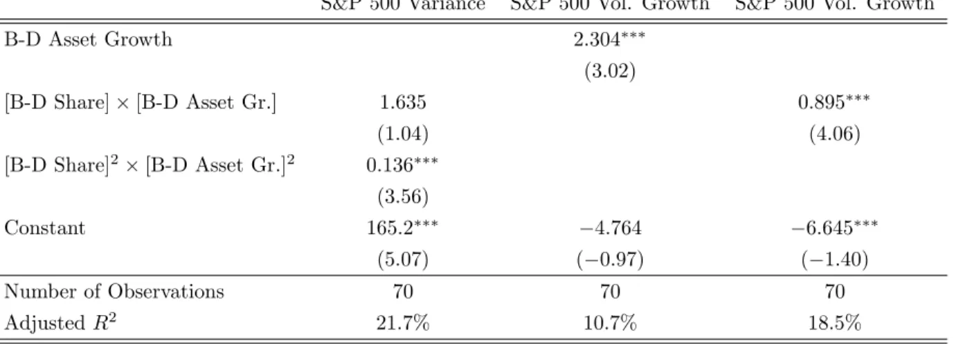
That is, high volatility of broker-dealer risk appetite should forecast high market variance. This prediction is investigated in Table 5.
Column (i) implements a contemporaneous version of (4:2) by running the realized S&P 500 variance on broker-dealer asset growth interacted withstand the
square of this variable The squared regressor is signi…cant at1%level, suggesting that high volatility of broker-dealer risk appetite is indeed associated with high market volatility. The regressors explain21:7%of the variation in market variance on an adjusted R2 basis. Running the regression with lagged right-hand-side variables yields no signi…cance at this horizon.
Columns (ii) and (iii) assess the e¤ect of broker-dealer asset growth on changes in S&P 500 volatility. The results show that broker-dealer asset growth is posi-tively associated with changes in market volatility; that is, market volatility in-creases at times of high broker-dealer risk appetite. The regressor is signi…cant at1% level and explains over 10% of the variation in volatility growth. Both the statistical signi…cance of the regressor and the economic power of the speci…ca-tion increase further when broker-dealer asset growth is interacted with their asset share.
4.3. Speculative Demand in the Futures Market
Finally, consider the impact of broker-dealer risk appetite on speculative activ-ity in commodactiv-ity futures. If changes in broker-dealer risk appetite drive expected commodity returns via the proposed mechanism, one should expect to see changes in speculators’open interest as broker-dealer risk appetite ‡uctuates. In partic-ular, an increase (decrease) in broker-dealer risk appetite that lowers insurance premia should be associated with an increase (decrease) in speculators’share of futures demand. In other words, when broker-dealer risk appetite increases, spec-ulators take more aggressive futures positions, which should be re‡ected in higher speculative open interest.
Column (i) of Table 6 demonstrates this e¤ect for crude oil: broker-dealer asset growth that bids up current crude oil prices (compresses risk premia) is associated with an increase in the speculator share of open interest. The result is signi…cant at1% level.
One can also demonstrate the direct e¤ect on contemporaneous crude oil re-turns. That is, an increase in broker-dealer risk appetite that increases the share of speculative demand in the futures market should be associated with a contem-poraneous increase in crude oil prices (compression of risk premia). This result is shown in column (ii).8
Similar results also obtain for other commodities with strong return pre-dictability. But note that commodities that have a negative loading on lagged broker-dealer risk appetite in Table 1 also have a di¤erent sign on the interaction terms of Table 6. This lends additional support to the prediction of the model that broker-dealer risk appetite determines expected commodity returns through its association with risk premia, where that risk premium may be positive or neg-ative depending on the covariance properties of the individual commodity (recall Figs. 3.1 3.2).
5. Cross-Sectional Prices of Risk
In order to investigate the signi…cance of broker-dealer risk appetite for the pricing of the cross-section of commodity returns, this section constructs and implements a cross-sectional asset pricing model with time-varying prices of risk.
8Note the similarity of these results to Campbell, Grossman and Wang (1993) where
risk-averse market makers accommodate selling pressure from liquidity traders. Their model predicts that an asset price decline on a high-volume day is more likely to be associated with an increase in the expected asset return than an asset price decline on a low-volume day. In the present framework, liquidity traders (hedgers) have to accommodate changes in broker-dealer (specu-lator) risk appetite by accepting a higher/lower futures price. A futures price increase is more likely to be associate with an increase in broker-dealer risk appetite when speculative activity is increasing than when speculative activity is decreasing.
5.1. Cross-Sectional Asset Pricing Approach
Letrit+1 be the excess return on a position in commodityi. Denoting the pricing kernel by Mt+1=Mt, the expected excess return is:
Et
Mt+1
Mt
rt+1i = 0:
De…ne the commodity risk premium,
t= Covt
Mt+1=Mt
Et(Mt+1=Mt)
; rt+1i ; (5.1) and express the excess return in terms of two components:
rit+1 |{z} Excess Return = t |{z} Commodity Risk Premium + uit+1 |{z} Commodity Risk ; (5.2) whereEt uit+1 = 0.
In order to estimate the prices of risk t, assume the pricing kernel is
expo-nentially a¢ ne in a set of state variablesXt:
Mt+1 Mt = exp ln (rt) 1 2 0 t t 0tvt+1 ; t t = 0+ 1Xt; where Xt+1 = + Xt+ tvt+1; vec( t 0t) = S0+S1Xt;
and vt+1 N(0; Ik). Using Stein’s lemma for the commodity risk premium (5:1)
and de…ning it0 =Covt rt+1i ; Xt+1 t1, the pricing equation(5:2) becomes:
Following Adrian and Moench (2008), one can further decompose the commodity-speci…c risk into a systematic and idiosyncratic component to obtain:
rt+1i |{z} Excess Return = it0( 0+ 1Xt) | {z } Commodity Risk Premia + it0vt+1 | {z } Systematic Commodity Risk + it+1 |{z} Idiosyncratic Commodity Risk ; (5.3) whereei t+1 N(0;1) for all i.
5.2. Estimating Prices of Risk
The cross-sectional model in (5:3) is estimated by way of three-stage OLS re-gressions applied to the cross-section of 14 commodities discussed above. For simplicity, it is assumed that the commodity-speci…c betas i are constant over time. The steps of the estimation procedure are outlined in Adrian and Moench (2008).
Following the reduced-form factor model(2:11) from Section 2, let the vector of state variables be given by:
Xt = 0 B B B B @
S&P 500 Excess Return GSCI Spot Excess Return
[B-D Share] [B-D Asset Growth]
PC1 PC2 1 C C C C A ;
where the S&P 500 is a proxy for the returns on marketable assets (rtM), the GSCI Spot is a proxy for the returns on non-marketable securities (rN M
t ), and the
negative of broker-dealer asset growth is a proxy for the tightness of broker-dealer balance sheet constraint ( Mt t). PC1 and PC2 are the …rst two principal
com-ponents extracted from the cross-section of commodity prices: PC1 is interpreted
as an equally-weighted commodity price index. PC2 captures systematic variation
between di¤erent classes of commodities.
Before proceeding to the results, note what to expect based on Section 2’s theoretical formulation. The main prediction of (2:11) concerns the tightness of
broker-dealer balance sheet constraint Mt , which in the time-series regressions of
Section 3 was proxied by the negative of broker-dealer asset growth. Since the dynamics of prices of risk tare linked to the state variablesXt, the cross-sectional
model gives one an opportunity to investigate the prediction of the model that the price of non-marketable risk GSCIt is linked to broker-dealer asset growth. In particular, the model predicts that GSCIt has a signi…cant positive load on lagged
[B-D Share] [B-D Asset Growth]. Note also that the model in its current static form remains silent about whether the innovations to [B-D Share] [B-D Asset Growth], i.e. balance sheet risk, should be priced. For an intertemporal asset pricing model with broker-dealer balance sheet constraints, see Adrian, Etula and Shin (2009).
The estimates for the cross-sectional prices of risk are displayed in Table 7. Columns (i)-(v) give the loadings of the four prices of risk kt on a constant 0
and on the lags of the state variables l1. The associated t-statistics are based
on a bootstrap with 1000 iterations. There are two things to note: First, the price of non-marketable risk (on the second row) has a signi…cant positive loading on the tightness of broker-dealer balance sheet constraints, [B-D Share] [ B-D Asset Growth]. This con…rms the prediction of the model that the price of non-marketable risk is inversely linked to broker-dealer risk appetite. Second, the price of balance sheet risk (on the third row) has a signi…cant negative loading on the aggregate market return, suggesting that the price of balance sheet risk is high in economic downturns.
The signi…cance of the prices of risk of each state variable is tested in Column (v). The p-values in brackets show that all risk premia except for the price of marketable risk are signi…cant at 1% level. This is consistent with the …ndings of numerous previous studies, which suggest that systematic market risk is not signi…cant for the pricing of commodity returns.
-15 -10 -5 0 5 10 15 1990 1992 1994 1996 1998 2000 2002 2004 2006 2008
Price of Non-Marketable Risk
Figure 5.1: Price of GSCI spot commodity risk (Q3/1990-Q4/2007)
-15 -10 -5 0 5 10 15 1990 1992 1994 1996 1998 2000 2002 2004 2006 2008
Price of Balance Sheet Risk
factors of interest, non-marketable risk and balance sheet risk. Both series are highly volatile, which re‡ects the same time-variation in commodity risk premia that was found to generate forecastability of commodity returns in Section 2. Note the increase in the price of non-marketable risk at the end of 2007 as a result of decreasing broker-dealer risk appetite. The sharp increase in the price of balance sheet risk over the same period stemmed from a simultaneous decline in equity prices and a run-up in non-energy commodity prices.
In order to assess the signi…cance of individual commodities’loadings on the risk premia, column (i) of Table 8 tests the joint signi…cance of betas for each commodity. The bootstrapped p-values in brackets indicate that all commodities except for silver have statistically signi…cant loadings on the innovations of state variables. Column (ii) conducts similar tests for the commodity risk premia, which correspond to the currency-speci…c betas multiplied by the prices of risk. The risk premium is signi…cant at the 5% level for 7 out of 14 commodities, which apart from corn and soybeans coincide with the forecastable commodities in Tables 1A and 1B. The di¤erences stem from the cross-sectional restrictions imposed by the model.
Finally, column (iii) investigates the quality of the pricing model by testing the predictability of forecast residuals by lagged state variables. The tests of excess forecastability are signi…cant only for unleaded gasoline and cocoa, which suggests that the model does a good job in pricing the rest of the cross-section. That is, the observed predictability of commodity returns is largely explained by market-wide risks, which cannot be diversi…ed away in the cross-section of commodities.
This result is regarded as further con…rmation of the paper’s rationalization of the channel through which balance sheet constraints operate. As suggested in the theoretical model, the balance sheet constraint and the associated La-grange multiplier t have the e¤ect of varying the apparent risk preferences of
sheet constraints are relatively loose, enabling market participants to expand their balance sheet on the back of permissive funding conditions. In contrast, market stringency is associated with tighter balance sheet constraints and higher values of the associated Lagrange multiplier. The fact that the observed predictability is explained by market-wide risks is additional evidence for broker-dealer balance sheet constraints operating through shifts in risk appetite.
In sum, the cross-sectional evidence supports the paper’s view that the fore-castability of commodity returns uncovered in Table 1 is in fact a re‡ection of systematic changes in risk premia. As broker-dealer balance sheets expand, spec-ulators’ risk appetite increases. This decreases the risk premia that speculators demand for insuring hedgers against spot commodity risk in the futures mar-ket; i.e., it decreases the price of non-marketable risk. Conversely, as balance sheets contract, investor risk appetite decreases. This increases the risk premia speculators demand for taking on spot commodity risk, raising the price of non-marketable risk.
6. Conclusion
This paper shows that broker-dealer asset growth forecasts commodity returns at quarterly horizons, both in-sample and out-of-sample. The pattern emerged following the establishment of futures markets and strengthened in lock-step with broker-dealer asset growth. I rationalize the results in a simple pricing model where broker-dealers provide insurance to producers and end-users of commodi-ties in the futures market. To the extent that hedgers’ demand for insurance is independent of the ‡uctuations in dealer risk appetite, changes in broker-dealer risk appetite are in equilibrium re‡ected in expected commodity returns through their association with risk premia. The model is also consistent with other quantitative and qualitative features of the data.
fact a re‡ection of systematic changes in risk premia. Excess commodity returns are compensation for market-wide risks, which include systematic non-marketable risk and systematic broker-dealer balance sheet risk. The price of non-marketable risk ‡uctuates with broker-dealer risk appetite and the price of broker-dealer bal-ance sheet risk ‡uctuates with market conditions. These cross-sectional …ndings lend additional support to the view that broker-dealer balance sheet constraints operate through shifts in risk appetite.
In sum, the empirical and theoretical contributions of the paper may be re-garded as the …rst steps toward understanding the impact of broker-dealer risk appetite on commodity prices. The ‡uctuations in broker-dealer risk appetite seem to be the common thread that ties together commodity price movements with changes in risk premia. Thus, the documented forecastability of commod-ity returns may be accompanied by shifting risk premia that are consistent with forward-looking portfolio decisions of investors.
References
[1] Adrian, T. and H.S. Shin. 2008a. “Liquidity and Leverage.” Journal of Fi-nancial Intermediation, forthcoming.
[2] Adrian, T. and H.S. Shin. 2008b. “Financial Intermediaries, Financial Stabil-ity, and Monetary Policy.”Jackson Hole Economic Symposium Proceedings, Federal Reserve Bank of Kansas City, forthcoming.
[3] Adrian, T. and H.S. Shin. 2008c. “Financial Intermediary Leverage and Value-at-Risk.” Federal Reserve Bank of New York Sta¤ Report no. 338. [4] Adrian, T. and E. Moench. 2008. “ Pricing the Term Structure with Linear
Regressions.” Federal Reserve Bank of New York Sta¤ Report no. 340. [5] Adrian, T., Etula, E. and H. Shin. 2008. “Global Liquidity and Exchange
Rates.” Working Paper.
[6] Barberis, N., A. Shleifer and R. Vishny. 1998. “A Model of Investor Senti-ment.” Journal of Financial Economics 69:307–343.
[7] Bessembinder, H. 1992. “Systematic Risk, Hedging Pressure, and Risk Pre-miums in Futures Markets.” Review of Financial Studies 5:637–667.
[8] Bessembinder, H. and K. Chan. 1992. “Time-Varying Risk Premia and Forecastable Returns in Futures Markets.” Journal of Financial Economics 32:169–193.
[9] Black, F., 1976. “The Pricing of Commodity Contracts.”Journal of Financial Economics. 3:167–179.
[10] Breeden, D.T. 1980. “Consumption Risk in Futures Markets.” Journal of Finance 35:503–520.
[11] Campbell, J.Y., Grossman S.J. and J. Wang. 1993. “Trading Volume and Serial Correlation in Stock Returns.” The Quarterly Journal of Economics 108:905–939.
[12] Campbell, J.Y. and A.S. Kyle. 1993. “Smart Money, Noise Trading and Stock Price Behaviour.” The Review of Economics Studies 60:1–34.
[13] Carter, C.A., Rausser, G.C. and A. Schmitz. 1983. “E¢ cient Asset Portfolios and the Theory of Normal Backwardation.” Journal of Financial Economics 91:319–331.
[14] Clark, T.E. and K.D. West. 2006. “Using Out-of-Sample Mean Squared Pre-diction Errors to Test the Martingale Hypothesis.” Journal of Econometrics 135:155–186.
[15] Clark, T.E. and K.D. West. 2007. “Approximately Normal Tests for Equal Predictive Accuracy in Nested Models.” Journal of Econometrics 138:291– 311.
[16] Danielsson, J., Shin, H.S and J. Zigrand. 2008. “Endogenous Risk and Risk Appetite.” working paper, London School of Economics and Princeton Uni-versity.
[17] DeLong, J.B., Shleifer, A., Summers, L.H. and R. Waldmann. 1990. “Noise Trader Risk in Financial Markets.”Journal of Political Economy 98:703–738. [18] Erb, C.B., and C.R. Harvey. 2006. “The Strategic and Tactical Value of
Commodity Futures.” Financial Analysts Journal 62:69–97.
[19] Gorton, G. and K.G. Rouwenhorst. 2006. “Facts and Fantasies about Com-modity Futures.” Financial Analysts Journal 62:47–68.
[20] Grossman, S.J. and M.H. Miller. 1988. “Liquidity and Market Structure.” Journal of Finance 43:617–633.
[21] Hicks, J. 1939.Value and Capital. Oxford University Press. Cambridge, UK. [22] Hirschleifer, D. 1988. “Residual Risk, Trading Costs, and Commodity Risk
Premia.” Review of Financial Studies 1:173–193.
[23] Hirschleifer, D. 1989. “Determinants of Hedging and Risk Premia in Com-modity Futures Markets.” Journal of Financial and Quantitative Analysis 24:313–331.
[24] Hodrick, R.J. and S. Srivastava. 1984. “An Investigation of Risk and Return in Forward Foreign Exchange.”Journal of International Money and Finance 3:5–29.
[25] Hong, H. and J. Stein. 1999. “A Uni…ed Theory of Underreaction, Momentum Trading and Overreaction in Asset Markets.”Journal of Financial Economics 54:2143–2184.
[26] Jagannathan, R. 1985. “An Investigation of Commodity Futures Prices Using the Consumption-Based Intertemporal Capital Asset Pricing Model.”Journal of Finance 40:175–191.
[27] Keynes, J.M. 1930.A Treatise on Money, Vol II. Macmillan. London. [28] Kyle, A.S. 1985. “Continuous Auctions and Insider Trading.” Econometrica
53:1315–1336.
[29] Rogo¤, K. and V. Stavrakeva. 2008. “The Continuing Puzzle of Short Horizon Exchange Rate Forecasting.” Working Paper.
[30] Myers, S.C. and N. Majluf. 1984. “Corporate Financing and Investment De-cisions when Firms Have Information that Investors Do Not Have.” Journal of Financial Economics 13:187–221.
[31] de Roon, F.A., Nijman, T.E. and Veld, C. 2000. “Hedging Pressure E¤ects in Fufures Markets.” Journal of Finance 55:1437–1456.
[32] Shleifer, A. and R. Vishny. 1997. “The Limits of Arbitrage.” Journal of Fi-nance 52:35–55.
[33] Stoll, H. 1979. “Commodity Futures and Spot Price Determination and Hedg-ing in Capital Market Equilibrium.” Journal of Financial and Quantitative Analysis 14:873–894.
TABLE 1A: Forecasting Quarterly Futures Returns (Q3/1990 - Q4/2007)
Energy
Crude Oil Heating Oil U. Gasoline Natural Gas S&P 500 Excess Return -0.369* -0.299 -0.363 0.046
(-1.788) (-1.299) (-1.501) (0.101) B-D Asset Growth (Lag 1) -1.296*** -1.079*** -1.376*** -0.741
(-5.429) (-4.051) (-4.926) (-1.410) Constant 4.608*** 4.094** 4.793*** 3.565 (3.037) (2.418) (2.698) (1.061) # Observations 69 69 69 68 Adjusted R2 34.8% 22.0% 29.8% 0.0% Metals
Gold Silver Platinum Copper S&P 500 Excess Return -0.128 0.036 0.202 0.173
(-1.274) (0.198) (1.514) (0.834) B-D Asset Growth (Lag 1) -0.121 -0.413** -0.214 -0.449* (-1.045) (-1.982) (-1.385) (-1.875) Constant 1.490** 2.502* 2.032** 2.024 (2.022) (1.888) (2.070) (1.328) # Observations 69 69 69 69 Adjusted R2 2.0% 2.8% 2.2% 2.5% Agriculture
Wheat Corn Soybeans Cocoa Cotton Sugar S&P 500 Excess Return -0.197 -0.071 0.072 -0.601*** 0.245 -0.049 (-0.871) (-0.286) (0.329) (-3.129) (1.108) (-0.177) B-D Asset Growth (Lag 1) 0.478* 0.119 0.124 0.508** -0.225 -0.223
(1.833) (0.415) (0.492) (2.288) (-0.880) (-0.698)
Constant 0.888 0.835 0.597 0.342 0.070 0.700
(0.535) (0.458) (0.372) (0.242) (0.043) (0.344)
# Observations 69 69 69 69 69 69
Adjusted R2 2.3% -2.7% -2.4% 13.5% -0.5% -2.1%
TABLE 1B: Forecasting Quarterly Excess Spot Returns (Q3/1990 - Q4/2007)
Energy
Crude Oil Heating Oil U. Gasoline Natural Gas S&P 500 Excess Return -0.373* -0.429 -0.516* 0.620
(-1.801) (-1.628) (-1.744) (1.148) B-D Asset Growth (Lag 1) -1.294*** -1.206*** -1.131*** -0.328
(-5.403) (-3.964) (-3.306) (-0.525) Constant 3.639** 3.601* 3.501 1.039 (2.390) (1.862) (1.610) (0.262) # Observations 69 69 69 69 Adjusted R2 34.6% 22.7% 18.1% -0.9% Metals
Gold Silver Platinum Copper S&P 500 Excess Return -0.147 0.025 0.192 0.172
(-1.417) (0.141) (1.408) (0.821) B-D Asset Growth (Lag 1) -0.129 -0.387* -0.261* -0.397
(-1.071) (-1.918) (-1.657) (-1.636) Constant 0.464 1.487 1.183 0.771 (0.607) (1.159) (1.180) (0.500) # Observations 69 69 69 69 Adjusted R2 2.8% 2.5% 2.8% 1.3% Agriculture
Wheat Corn Soybeans Cocoa Cotton Sugar S&P 500 Excess Return 0.069 0.050 0.099 -0.513*** 0.077 -0.166 (0.273) (0.191) (0.408) (-3.095) (0.393) (-0.701) B-D Asset Growth (Lag 1) 0.583** 0.208 0.166 0.472** -0.196 -0.198
(1.993) (0.687) (0.594) (2.465) (-0.861) (-0.724)
Constant -0.695 -0.451 -0.540 -0.605 -0.559 0.046
(-0.374) (-0.234) (-0.304) (-0.496) (-0.386) (0.027)
# Observations 69 69 69 69 69 69
Adjusted R2 3.5% -2.1% -2.0% 14.0% -1.8% -1.1%
TABLE 1C: Forecasting Quarterly Excess Index Returns (Q3/1990 - Q4/2007)
GSCI (Fut.) GSCI (Spot) DJCI (Fut.) DJ Corp. Bond Index S&P 500 Excess Return -0.176 -0.155 -0.093 0.620
(-1.18) (-1.07) (-0.95) (1.148) B-D Asset Growth (Lag 1) -0.567*** -0.584*** -0.364*** -0.328
(-3.28) (-3.48) (-3.20) (-0.525)
Constant 1.907* 1.696 0.791 1.039
(1.73) (1.59) (1.09) (0.262)
# Observations 69 69 69 69
Adjusted R2 15.4% 16.6% 13.8% -0.9%
T ABL E 2A: Q uarter ly In-Sample Regr essi on s (Q3/1 990 -Q 4/200 7) Cr ud e Oil Excess Retur n (i) (ii) (iii ) (i v) (v) (vi ) (v ii) (vii i) B-D Ass et Gr . (Lag 1) 1 : 361 1 : 363 1 : 341 1 : 288 1 : 284 1 : 180 1 : 185 1 : 152 ( 5 : 944) ( 5 : 990) ( 5 : 826) ( 5 : 718) ( 5 : 980) ( 5 : 231) ( 5 : 274) ( 5 : 046) VIX (L ag 1) 0 : 109 0 : 146 0 : 123 0 : 359 0 : 352 0 : 328 ( 0 : 527) ( 0 : 690) ( 0 : 567) ( 1 : 403) ( 1 : 371) ( 1 : 280) In te re st Rat e (Lag 1 ) 5 : 071 10 : 301 3 : 627 4 : 181 5 : 963 ( 1 : 317) ( 1 : 986) ( 0 : 492) ( 0 : 568) ( 0 : 810) Yi el d S pr . (Lag 1) 8 : 080 1 : 675 1 : 326 0 : 499 ( 1 : 475) (0 : 189) (0 : 149) (0 : 057) Di v. Yield (Lag 1) 5 : 262 5 : 441 5 : 167 ( 1 : 328) ( 1 : 267) ( 1 : 232) In‡ at ion (Lag 1) 2 : 148 0 : 480 (0 : 198) (0 : 044) Hedging Pr es. (Lag 1) 0 : 105 (1 : 211) Dep. V ar . (Lag 1) 0 : 023 0 : 021 0 : 005 0 : 020 0 : 061 0 : 055 0 : 182 (0 : 307) (0 : 273) ( 0 : 067) ( 0 : 264) ( 0 : 758) ( 0 : 660) ( 1 : 412) Cons tan t 4 : 028 4 : 030 6 : 027 11 : 435 21 : 726 23 : 150 22 : 792 24 : 770 (2 : 708) (2 : 685) (1 : 513) (1 : 892) (2 : 323) (2 : 418) (2 : 317) (2 : 501) # Obs er v a tions 68 6 8 68 68 68 68 68 68 Adj usted R 2 33 : 96% 33 : 01% 32 : 22% 32 : 90% 33 : 45% 34 : 98% 33 : 93% 35 : 06% Not e: Robus t t-stat istics in p a ren thes es; *** p < 0.0 1, ** p < 0.0 5, * p < 0.1 .
T ABLE 2B: Qua r terl y In-S ample Regres sions (Q 3/1990 -Q4/ 2007) S&P GSCI E x ces s R etu r n (i) (ii) (iii ) (i v) (v) (v i) (vii ) (vi ii) B-D Ass et Gr . (Lag 1) 0 : 524 0 : 518 0 : 499 0 : 453 0 : 454 0 : 400 0 : 403 0 : 409 ( 3 : 682) ( 3 : 527) ( 3 : 335) ( 2 : 996) ( 3 : 163) ( 2 : 615) ( 2 : 606) ( 2 : 662) VIX (L ag 1) 0 : 104 0 : 147 0 : 134 0 : 276 0 : 269 0 : 261 ( 0 : 669) ( 0 : 968) ( 0 : 867) ( 1 : 349) ( 1 : 293) ( 1 : 239) In te re st Rate (Lag 1 ) 5 : 300 9 : 360 5 : 494 5 : 964 7 : 555 ( 1 : 929) ( 2 : 473) ( 1 : 024) ( 1 : 082) ( 1 : 330) Yi eld S pr. (Lag 1) 6 : 180 0 : 511 0 : 796 1 : 811 ( 1 : 620) ( 0 : 078) ( 0 : 120) ( 0 : 271) Di v. Yield (Lag 1) 3 : 100 3 : 261 3 : 017 ( 1 : 165) ( 1 : 203) ( 1 : 119) In‡ at ion (Lag 1) 1 : 897 1 : 030 (0 : 267) (0 : 144) Hed g ing Pr es. (Lag 1) 0 : 071 (1 : 430) Dep. V ar . (Lag 1) 0 : 039 0 : 030 0 : 022 0 : 050 0 : 089 0 : 080 0 : 216 (0 : 429) (0 : 318) ( 0 : 222) ( 0 : 510) ( 0 : 822) ( 0 : 709) ( 1 : 481) Cons tan t 1 : 802 1 : 784 3 : 692 9 : 468 17 : 477 18 : 518 18 : 157 20 : 112 (1 : 738) (1 : 714) (1 : 293) (2 : 279) (2 : 494) (2 : 630) (2 : 434) (2 : 711) # Obs er v a tions 68 6 8 68 68 68 68 68 68 Adj usted R 2 13 : 16% 11 : 99% 11 : 26% 15 : 15% 16 : 40% 17 : 58% 16 : 28% 18 : 06% Not e: Ro b us t t-stat istics in p a ren thes es; *** p < 0.0 1, ** p < 0.0 5, * p < 0.1 .
TABLE 3A: Quarterly Out-of-Sample Regressions (Q2/1995 - Q4/2007)
Crude Oil Excess Return (rt+1)
Normal (DMW) Clark-West Adjusted Restricted Model (r) Unrestricted Model (u) M SEr M SEu M SEr (M SEu adj:)
(1) Etrt+1= 0 Etrt+1= 0t+ 1txt 58:72 110:75 [0:041] [0:004] (2) Etrt+1= 0t Etrt+1= 0t+ 1txt 68:49 121:20 [0:029] [0:004] (3) Etrt+1= 0t+ 1trt Etrt+1= 0t+ 1trt+ 2txt 69:09 122:51 [0:032] [0:005] Number of Observations 48 48
Note: Bootstrapped p-values in brackets: *** p<0.01, ** p<0.05, * p<0.1.
TABLE 3B: Quarterly Out-of-Sample Regressions (Q2/1995 - Q4/2007)
S&P GSCI Excess Return (rt+1)
Normal (DMW) Clark-West Adjusted Restricted Model (r) Unrestricted Model (u) M SEr M SEu M SEr (M SEu adj:)
(1) Etrt+1= 0 Etrt+1= 0t+ 1txt 8:120 16:449 [0:159] [0:026] (2) Etrt+1= 0t Etrt+1= 0t+ 1txt 12:623 19:649 [0:062] [0:014] (3) Etrt+1= 0t+ 1trt Etrt+1= 0t+ 1trt+ 2txt 10:710 18:417 [0:098] [0:021] Number of Observations 48 48
TABLE 4: Risk Appetite and Market Risk Premia
VIX Premium VIX Premium VIX Prem. VIX Prem. CDX
B-D Asset Growth 0:206 0:397 ( 3:06) ( 4:12) [B-D Share] [B-D Asset Gr.] 0:090 0:138 0:276 ( 4:78) ( 4:95) ( 2:07) Constant 5:376 5:616 0:845 1:045 51:578 (12:44) (13:97) (1:37) (1:75) (16:21) # Observations 70 70 70 70 17 AdjustedR2 10:8% 24:1% 18:8% 25:5% 16:4%
Note: Bootstrapped t-statistics in parentheses; *** p <0.01, ** p<0.05, * p<0.1.
TABLE 5: Risk Appetite and Market Volatility
S&P 500 Variance S&P 500 Vol. Growth S&P 500 Vol. Growth
B-D Asset Growth 2:304 (3:02) [B-D Share] [B-D Asset Gr.] 1:635 0:895 (1:04) (4:06) [B-D Share]2 [B-D Asset Gr.]2 0:136 (3:56) Constant 165:2 4:764 6:645 (5:07) ( 0:97) ( 1:40) Number of Observations 70 70 70 AdjustedR2 21:7% 10:7% 18:5%
T ABLE 6: Ri sk App etite and Sp eculati v e Activit y in the F utures Mar k et Sp ecu lator s’ Share of OI Crud e Oi l E x cess Ret. B-D Ass et Gr o wth 0 : 297 B-D Ass et Gr o wth 0 : 33 (1 : 81) (1 : 04) Crude O il Exce ss Return 0 : 104 Sp ecu lator s’ Share of OI 0 : 299 (1 : 74) (1 : 28) [ B-D Ass et Gr . ] x [ Crude Ret. ] 0 : 022 [ B-D Ass et Gr . ] x [ Sp ecu lator s’ O I ] 0 : 061 (2 : 98) (2 : 26) Cons tan t -0 : 720 Cons tan t 0 : 489 (0 : 77) ( 0 : 27) # Obs er v a tions 69 # Obs erv a tions 69 Adj usted R 2 14 : 1% Adj usted R 2 9 : 3% Not e: t-stati st ics in p ar en the ses ; *** p < 0.0 1, ** p < 0.0 5, * p < 0.1 .
T ABLE 7: C ross -Sectional Pri ces of Ris k Res id ual 0 S & P 50 0 1 GS C I 1 B D 1 P C 1 1 P C 2 1 0 = S & P 50 0 1 = ::: = P C 2 1 = 0 S&P 5 00 E x cess Return 2 : 065 0 : 025 0 : 222 0 : 208 0 : 722 1 : 241 [0 : 152] ( 1 : 65) (0 : 15) (1 : 87) ( 2 : 78) ( 1 : 75) (1 : 79) G S CI S p ot Exces s Retu rn 0 : 093 0 : 126 0 : 118 0 : 150 0 : 595 0 : 427 [0 : 000] ( 0 : 17) (1 : 69) ( 2 : 47) (4 : 36) (3 : 28) ( 1 : 49) [ B-D S har e ] [ B-D Ass et Gr . ] 0 : 721 0 : 570 0 : 185 0 : 082 0 : 185 2 : 130 [0 : 000] (0 : 84) ( 5 : 70) ( 2 : 86) (1 : 43) (0 : 63) (4 : 62) PC 1 0 : 198 0 : 020 0 : 003 0 : 003 0 : 014 0 : 070 [0 : 001] ( 2 : 83) (2 : 13) (0 : 47) ( 0 : 72) (0 : 47) ( 1 : 72) PC 2 0 : 058 0 : 017 0 : 003 0 : 008 0 : 053 0 : 100 [0 : 000] ( 0 : 97) (2 : 31) (0 : 54) ( 2 : 52) (2 : 72) ( 2 : 95) Not e: Bo otstrapp ed t-s tatisti cs in paren th ese s, p-v al u es in brac k ets ; *** p < 0.0 1, ** p < 0.0 5, * p < 0.1 .
T ABL E 8: S ign i… cance of ’s , 0 ’s and Excess Predictabil it y T est Ass et S & P 50 0 = B D = ::: = P C 2 = 0 0 0 = 0 B D 1 = ::: = 0 P C 2 1 = 0 Pred ic tab ilit y of F o rec a st Residu al s Crude O il [0 : 000] [0 : 000] [0 : 319] Heati n g O il [0 : 000] [0 : 000] [0 : 552] U. G asoline [0 : 000] [0 : 000] [0 : 055] Nat u ral Gas [0 : 001] [0 : 640] [0 : 748] G old [0 : 007] [0 : 582] [0 : 114] Silv er [0 : 153] [0 : 544] [0 : 405] Plati n um [0 : 000] [0 : 312] [0 : 018] Copp er [0 : 026] [0 : 855] [0 : 245] Wh eat [0 : 001] [0 : 047] [0 : 379] Cor n [0 : 000] [0 : 000] [0 : 920] So yb ea n s [0 : 000] [0 : 004] [0 : 537] Co coa [0 : 030] [0 : 021] [0 : 049] Cott on [0 : 000] [0 : 243] [0 : 273] Su ga r [0 : 007] [0 : 376] [0 : 939] Not e: Bo otstrapp ed p -v al u es in b rac k et s; ** * p < 0.0 1, ** p < 0.0 5, * p < 0.1 .