Statistical Downscaling Output GCM Modeling with Continuum Regression and Pre-Processing PCA Approach

(1)

AbstractOne of the climate models used to predict the climatic conditions is Global Circulation Models (GCM). GCM is a computer-based model that consists of different equations. It uses numerical and deterministic equation which follows the physics rules. GCM is a main tool to predict climate and weather, also it uses as primary infor-mation source to review the climate change effect. Statis-tical Downscaling (SD) technique is used to bridge the large-scale GCM with a small scale (the study area). GCM data is spatial and temporal data most likely to occur where the spatial correlation between different data on the grid in a single domain. Multicollinearity problems require the need for pre-processing of variable data X. Continuum Regression (CR) and pre-processing with Principal Compo-nent Analysis (PCA) methods is an alternative to SD modelling. CR is one method which was developed by Stone and Brooks (1990). This method is a generalization from Ordinary Least Square (OLS), Principal Component Regression (PCR) and Partial Least Square method (PLS) methods, used to overcome multicollinearity problems. Data processing for the station in Ambon, Pontianak, Losarang, Indramayu and Yuntinyuat show that the

RMSEP values and R2predict in the domain 8x8 and 12x12 by

uses CR method produces results better than by PCR and PLS.

KeywordsCR, PCA, PCR, PLS, SD, GCM

I.INTRODUCTION

ecently General Circulation Models (GCM) is recognized by many people as important tools in understanding the climate system. But many scientific communities expressed some dissatisfaction, because it has produced an inadequate space scale forecast [14]. One effort to overcome these problems is the use of Statistical Downscaling (SD) method [4]. The main advantage of this method is inexpensive computation and easy application in many output simulations and experiments which based on GCM.

Some SD methods for many climate studies were developed in high latitude countries, whereas in low latitude region (such as Indonesia) is still very limited [4][14].There are SD methods for generating large scale and local scale model relathionship such as based on region or spatial, temporal, dependent variable, independen variable, and statistical methods. SD method often used are classical or multiple regression [1, 2], canonical correlation [2, 16], Singular Value Decomposition (SVD) [11], and non linear approach such as artificial neural network [3]. SD models

1

Sutikno and Setiawan are with Department of Statistics, FMIPA, Institut Teknologi Sepuluh Nopember, Surabaya, 60111, Indonesia. E-mail: [email protected].

2

Hendy Purnomoadi is Student of Statistics Department Master Program, FMIPA, Institut Teknologi Sepuluh Nopember, Surabaya, 60111, Indonesia.

developed in Indonesia are Haryoko (2004) and Wigena & Aunuddin (2004) [13], but it did not consider spatial however correlation, autocorrelation case and problems of non linear structure data.

The problems that arise in the SD method are how to determine domain (grid) and dimensions reduction, how to obtain an independent variable that may explain the diversity of the dependent variable, and obtain appropriate statistical methods of data characteristics that can describe the relationship between independent variables and the dependent variable, accommodate how to employ extreme events. The method often used for pre-processing are the Principal Component Analysis (PCA), Discrete Wavelet Transform (TWD), Robust Principal Component Analysis (ROBPCA), and Kernel PCA; furthermore, Continuum Regression (CR) is also a model for the dependent variable with variable pre-processing. It is one potential method to overcome the multicollinearity.

The purpose of this study is to compare the performance of CR, PCR and PLS with PCA pre-processing by Root Mean Square Error Prediction (RMSEP) and R2predict criteria.

II.THEORIES

A. Principal Components Analysis (PCA)

PCA is a procedure to reduce the dimension of data by transforming the original variables correlated to a set of new uncorrelated variables. New variables are told as a Principal Component (PC) [6].

PC can be obtained from the eigenvalue-eigenvector pairs of covariance matrix or correlation matrix. First, standardization of data is done first when a unit of data between variables are not equal. It isessensially done so that the dominance of one or two variables in a PC can be avoided. If Σ is a variance-covariance matrix from random vector XT=[X1,X2,…, Xp]. Σ is obtained from the method of Maximum Likelihood Estimation (MLE) with the formula in Equation (1).

(

)(

)

T

i n

i

i x

x

n µ µ

Σ − −

−

=

∑

=1

1

1 (1)

∑

=

= n

i i x n 1

1

µ (2)

Z2=e2ΤX= e12X1 + e22X2 + . . . + ep2Xp ….

Zp=eрTX = e1pX1 + e2pX2 + . . . + eppXp (3) with:

Z1 = first PC, which has the largest variance

Z2 = second PC, which has the second largest variance Zp = p-th PC, which has p-th largest variance

X1 = the origin of the first variable

Statistical Downscaling Output GCM Modeling

with Continuum Regression and Pre-Processing

PCA Approach

Sutikno

1

, Setiawan

1

, and Hendy Purnomoadi

1

2

(2)

X2 = the origin of the second variable Xp = the origin of the p-th variable

PC models i-th can also be written with the notation Zi= eiΤX where,

i = 1, …,p and: i

T i

i e e

Z

Var( )= Σ , _i₌₁_,₂_,_...,_p (4)

, = ∑ , ≠ (5)

PC are not correlated and have the same variance with eigenvalues of Σ, then,

( )

tr

( )

1 2 ... p p

1 i Var Xi pp

... 22

11+σ + +σ = ∑₌ = Σ =λ +λ + +λ

σ (6)

when the total population variance is,

σ11+ σ22+ σpp= λ1+ λ2+ … + λp, then,

total variance can be explained by the i-th PC =

p 2 1

i

...+λ

+ λ +

λ λ (7)

if the PC is taken as k, where (k<p), then, =

p 2 1

k 2 1

... ...

λ + + λ +

λ +λ + +λ

λ ₍₈₎

Furthermore, when it is employed used the beginning is the covariance matrix of standardized data, due to the main diagonal matrix containing the value of one, then the total population variance for the standardized variable is p, representing the diagonal matrix elements

ρ,then total variance can be explained by the i-th PC =

p i

λ ₍₉₎

B. Partial Least Square (PLS)

PLS method is a statistical method to generalize and combine the methods of factor analysis, PCA, and multi-ple regressions. The purpose of PLS is to form a compo-nent that can capture information from the independent variable to predict the dependent variable.

PCA focuses on diversity in the independent variables, while PLS focuses on the covariance between indepen-dent variables and the depenindepen-dent variable. The model from PLS methods consists of external and internal rela-tions. External relations in the PLS is an individual and group relationships.

C. Continuum Regression (CR)

CR is a regularized regression estimation methods (a set), and used to handle the collinearity or multicol-linearity problems, which means there are approaches a linear relationship between the independent variables. CR is developed from the OLS, PCR, and PLS regres-sion.

Based on the following linear regression model:

y = Xβ + ε (10)

with independent variable X (size nxp) that has been centered and the dependent variable y (size nx1) is the vector that has been centered. In the case of multicol-linearity show that X is not full rank matrix. Consequent-ly, matrix XTX is (almost) singular.

In a linear weighted regression model, mathematical formula can be written as follows, by maximizing

(

)

Sw w y

s w

x w

x

w i

T i

T T

n

i

i T n

i i n

i w

y y

r ₂

2

1

2 1

2

1 2

) (

= 

    

   

 

= =

∑

= =

= (11)

With x_іis the observation vector with the i-th inde-pendent variables (i=1,2, ..., n) size (px1),s = XTyand S = XTX.

PCR principle is to maximize:

(

w x

)

wTSw

i T n

i w

S =

∑

=

2

1

(12) From formula (12) shows that the basic principle of PCR is used to maximize the variance of the independent variable X thus a new variable is formed in the form of several major components which are linear combinations of original variables (X). Furthermore, the dependent variable y is regressed with several major components using multiple linear regression techniques.

PLS regression principleis to maximize :

( )

2 2

1

s w x

w _ ₌ T

  

 

=

∑

=

n

i

i T i

w y

S (13)

Then from formula (13) it can be seen that PLS regression principle is used to maximize the covariance between the dependent and independent variables.

New variable in CR are written as follows in Equation (14).

y = Thξ + ε, with Th = XW (14)

And Wh = ( w1,w2,….,wh ) is a matrix containing h columns variable with h < p and called as weighting ma-trix.

Stone and Brooks (1990) formulated the following weighting matrix as [4]:

= arg , ! "#!⁄ %&'

( (15) with constrains║W2║=1 and Cov(Xwi, Xwj) = 0 for і < j while the parameter adjustment δ is a real number 0 ≤δ

≤1.

Another alternative is a formula developed by Malpass (1996) as follows [7] :

= arg , * !#+!, _{#"* !}

(

(16) From the formula (15) made a general formula as follows:

(

_T _T

) (

2 _T _T

)

[(/(1 ))1]

Xw X w y X w

G= δ −δ − (17)

Furthermore it was called as Stone methods. From the formula (16) can be made into :

(

T T

)

(22 4 )

(

T T

)

(12)

Xw X w y

X w G

2 ₋₊_δ

δ − δ +

= (18)

Furthermore this formula was called the Portsmouth methods [7].

The formula is a generalization of the OLS, PCR and PLS with the following forms of linkage:

1. For δ = 0, then G = (wTs)2(wTSw)-1 this formula is equivalent to Equation (11), thats mean, if δ = 0 CR is OLS.

2. Forδ = 0.5, thenG = (wTs)2 this formula is equivalent to Equation (12), so that, if δ = 0.5CR is PLS

3. Forδ = 1, thenG = (wTSw) this formula is equivalent to Equation (13), so that, if δ = 1 CR is PCR.In other words, OLS, PCR and PLS are a special form of CR. Estimation of regression parametersξ in the Equation (14) performed using least squares method is formulated as follows:

(

T T

)

T y

ξ T

h h T h h

1 ,

ˆ ₌ −

δ (19)

h , h h

, XW ξˆ

yˆ_δ = _δ

( )

T T T y W

βˆ T

h 1 h T h h h ,

−

(3)

where δ is an adjustment parameters and h is the number of components.

D. Goodness Model

Common measuring using good us model has the coef-ficient of determination R2 describing the goodness of prediction.

2 n

1 i

i 2 n

1 i

i

Total Error 2

predict

) Y Y (

) Y Yˆ (

SS SS 1 R

∑

= =

− − =

− =

(21)

R2predict = coefficient determination

-. = mean of the observed data Yi = actual values

Ŷ = prediction values Another criteria is :

(

)

n Yˆ Y RMSEP

n

1 i

2 i i

∑

= −

= (22)

RMSEP = Root Mean Square Error Prediction n = number of sample

Yi = actual values of out sample data

Ŷ = prediction values of out sample data E. General Circulation Model (GCM)

GCM is climate models based on computer. It uses numerical and deterministic equations which follow the physics rules. GCM is the main tool to predict or forecast climate and weather, understanding climate and climate change studies. According to [15], GCM is a major tool in the study of diversity and climate change. GCM climate models have the form of outcome-grid grid size 100-500 km, according to the latitude and longitude. This model can be used to predict changes in weather elements [16]. However, GCM is a global information, so it is difficult to obtain direct information on the local scale. But the GCM is still possible to obtain information about local or regional scale when the downscaling tech-nique is used [13].

Downscaling is defined as an effort to connect between global-scale circulation variables (explanatory variables) and local scale variables (dependent variable) [9]. To bridge the large-scale GCM with a smaller scale (the study area), it use SD. SD is a process of downscaling which static, data on large-scale grid-grid in a certain time period and used as the basis for determining the da-ta on a smaller scale grid [13].

SD approach uses regional or global data to obtain the functional relationship between the local scaleto global scale GCM. In general, the relationship is expressed by: Y = f(Z) + ε

with,

Y :dependent variable (rainfall)

Z :independent variable (compound

of the reduction

result of spatial (latitude and longitude) GCM

variables

ε : error

III.METHOD

This research uses secondary data obtained from GCM

output model CSIRO-Mk3, resolution of grid latitude and longitude 1,8650 x 1,8750. It can be downloaded at http://www-pcmdi.llnl.gov/ipcc. GCM domains are 3x3, 8x8 and 12x12 from five stations. Pontianak station uses the datafrom 1947-1990. Ambon Station use data in 1900-1940, Losarang Station in 1967-2000, Indramayu Station in 2000, and Yuntinyuat Station in 1974-2000. Monthly rainfall data are obtained from Badan Meteorologi Klimatologi dan Geofisika (BMKG).

Independent variables are CSIRO Mk3 outcomes. They are precipitable water (PRW), sea level pressure (SLP), meridional wind component (VA), zonal component (UA), geopotential height (ZG), and specific humidity (HUSS). The height (level) is 850 hPa, 500 hPa and 200 hPa. The dependent variable is the monthly rainfall data from five stations.

There two criteria to get the performance of CR, PCR and PLS with PCA dimension reduction, namely: RMSEP and R2predict. The best model is the model with small RMSEP and high R2predict.

IV.RESULT AND DISCUSSION

A. Pre-processing SD Modeling

The first step in the SD modeling is by means of dimension reduction, called the pre-processing of data. Spatial dimension reduction is performed on the latitude and longitude or grid and called on all variables in every level and every domain. In this case, each grid is an independent variable, so the domain 3x3, 8x8 and 12x12 are respectively sequenced 9, 64, and 144 variables and they will be reduced.

B. PCA Method

The procedure for preparing the main components with the PCA is done through three steps: first, getting the variance-covariance matrix, second, obtaining eigen-values and eigenvector matrix of variance-covariance based on the first step, and finally conducting a linear combination of eigenvector with the origin data to obtain the main components.

Through the steps using the PCA method, it is obtained the number of principal components and cumulative variance (CV) for GCM variables, listed in Table 1 until Table 3.

Based on Table 1 the components produced by GCM variables using the PCA method have CV greater than or equal to 85%. Domain 3x3 is using one main component, except for variable HUSS. HUSS variable use three main components, which subsequently written HUSS1, HU-SS2, and HUSS3. Domain 8x8 have main component which ranges from one to three, except HUSS variable that uses six main components (HUSS1, HUSS2, HUSS3, HUSS4, HUSS5, and HUSS6). Domain 12x12 has not more than four main components, except for va-riable HUSS and VA500.

In general, the variables on the level surface have main components which are comparable to increasing domain size, except for SLP variable.

(4)

tianak station can be seen in Table 2 and Table 3. C. CR, PCR, and PLS Method

SD modeling by means of CR, PCR and PLS methods uses independent variable produced from dimension re-duction in PCA method. It was done in Ambon station (type local rain), Pontianak station (type equatorial rain), and Losarang, Indramayu, and Yuntinyuat station (type of monsoon rains). Ambon has total of independent variables used in the domain 3x3 are 16 variables, in the domain 8x8 are 28 variables, and in the domain 12x12 are 39 variables. Pontianak has total of independent variables used in the domain 3x3 are 20 variables, in the domain 8x8 are 40 variables and in the domain 12x12 are 53 variables.

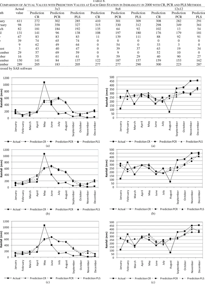
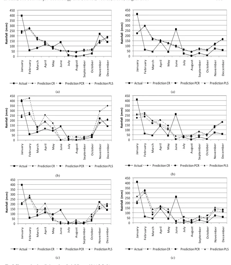
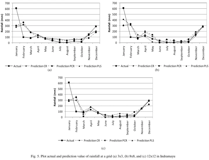
Losarang, Indramayu, and Yuntinyuat have total independent variables used in the domain 3x3 are 19 variables, in the domain 8x8 are 34 variables and in the domain 12x12 are 50 variables. The comparison of actual values and prediction value of rainfall variable each station and each grid is shown in Table 4 - Table 8. It also can be seen in Fig. 1 – Fig. 5. Indramayu has better results than other stations. The prediction and actual value have relatively small difference. But in other stations, the comparison has not been satisfactory, because the prediction value is still far from the actual value.

RMSEP values and R2predict from SD modeling use Continuum Regression method, PCR, and PLS in Ambon, Pontianak, Losarang, Indramayu and Yunti-nyuat Station with domains 3x3, 8x8 and 12x12 as seen in Table 9. In domain 3x3, PLS method has RMSEP smaller and R2predict higher than CR and PCR method. In domain 8x8, PLS method has RMSEP smaller and CR method has R2predict higher than others. In domain 12x12, CR method has RMSEP smaller and R2predict higher than others. So, it can be concluded that CR method has good performance than PCR and PLS method.

IV.CONCLUSION

CR with PCA pre-processing can be used to overcome multicollinearity problems at SD modeling to forecast the monthly rainfall in Ambon, Pontianak, Losarang, In-dramayu and Yuntinyuat Station on grid 3x3, 8x8, and 12x12.

CR method show better results method of PCR and PLS Regression. It can be seen from the average value of RMSEP and R2predict on each method and each grid.

ACKNOWLEDGMENT

Thanks go to DP2M DG DIKTI DEPDIKNAS who has supported this research through Hibah Penelitian

Strategis Nasional the year 2009.

REFERENCES

[1] A. Busuioc, D. Chen, C. Hellström, 2001, “Performance of

statistical downscaling models in gcm validation and regional climate change: application for Swedish precipitation”, Int. J.

Climatology, Vol. 21, pp. 557-578.

[2] A. Busuioc, H. Von Stroch, R.Schnur, 1999, “Verification of

GCM-generated regional seasonal precipitation for current climate and of statistical downscaling estimates under changing climate conditions”, Journal of Climate,Vol. 12, pp. 258-272.

[3] R. G. Crane, B. C. Hewitson, 1998, “Doubled CO2 precipitation

changes for the Susquehanna basin: downscaling from GENESIS general circulation model”, Int. J. Climatology 18, pp. 65-76.

[4] F. Giorgi, B. Hewitson, J.Christensen, M. Hulme, H. Von

Stroch, P.Whetton, R.Jones, L.Mearns, C.Fu, 2001, “The scientific basis”, Contribution of Working Group I to the Third

Assesment Report of the Intergovernmental Panel on Climate Change IPCC. University Press. Cambrige.UK.

[5] U. Haryoko, 2004, “Pendekatan reduksi dimensi luaran GCM

untuk penyusunan model statistical downscaling [tesis]”, Sekolah Pascasarjana, Institut Pertanian Bogor.

[6] R. A. Johnson, and D. W. Wichern, 2002, Applied Multivariate

Statistical Analysis, Vol. 5. New Jersey: Prentice Hall.

[7] J. Mallpass, 1996, Improved Mathematical Methods for Drugs

Design: Continuum Regression SAS Macro, University of

Portsmouth.

[8] M. Stone, R. J. Brooks, 1990, “Continuum Regression:

cross-validated sequentially constructed prediction embracing ordi-nary least squares, partial least squares, and principal component regression (with discussion)”, Journal of the Royal Statistical

Society Series B, Vol. 52, pp. 237-269.

[9] Sutikno, 2008, “Statistical downscaling luaran GCM dan

peman-faatannya untuk peramalan produksi padi”, Disertasi, Bogor, Program Pascasarjana, Institut Pertanian Bogor.

[10] R. M. Trigo, J. P. Palutikof, 2001, “Precipitation scenario over

Iberia. A comparison between direct GCM output and different downscaling techniques”, Journal of Climate, Vol. 14, pp. 4422-4446.

[11] C. B. Uvo, J. Olsson, O. Morita, K. Jinno, A. Kawamura, K.

Nishiyama, N. Koreeda, T. Nakashima, 2001, “Statistical atmos-pheric downscaling for rainfall estimation in Kyushu Island Japan”, Hydrology and Earth System Sciences, Vol. 5, pp. 259-271.

[12] A. H. Wigena, 2006, “Pemodelan statistical downscaling dengan

regresi projection pursuit untuk peramalan curah hujan bulanan”,

Disertasi, Program Pascasarjana, Institut Pertanian Bogor.

[13] A. H.Wigena, Aunuddin, 2004, “Aplikasi projection pursuit dan

jaringan syaraf tiruan dalam pemodelan statistical downscaling”,

Jurnal Statistika UNISBA, Vol. 4, No. 2, pp. 7-10.

[14] R. L. Wilby, S. P.Charles, E. Zorita, B. Timbal, P. Whetton, L.

O. Mearns, 2004,“Guidelines foe use of climate scenarios deve-loped from statistical downscaling methods”, http://www.ipcc-ddc.cru.uea.ac.uk/guidelines/ [8 Desember 2008].

[15] E. Zorita and H.von Storch, 1999, “The analog method as a

simple statistical downscaling technique: comparison with more complicated method”, Journal of Climate, Vol. 12, pp. 2474-2489.

[16] H. Von Strorch, E. Zorita, U. Cubash, 1993, “Downscaling of

(5)

TABLE 1.

TOTAL PCOPTIMAL AND CUMULATIVE VARIANCE (CV) FROM OUTCOME VARIABLES OF GCM BY USING PCAMETHOD

No. Variable Domain 3x3 Domain 8x8 Domain 12x12

PC CV PC CV PC CV

1 HUSS 3 0.898 6 0.853 10 0.854

2 HUS200 1 0.977 1 0.864 2 0.917

3 HUS500 1 0.967 2 0.926 2 0.856

4 HUS850 1 0.937 2 0.903 3 0.884

5 PRW 1 0.923 2 0.876 3 0.899

6 SLP 1 0.975 1 0.880 2 0.959

7 UAS 1 0.949 2 0.916 3 0.875

8 UA200 1 0.985 1 0.911 2 0.973

9 UA500 1 0.918 2 0.887 0.903

10 UA850 1 0.983 1 0.859 2 0.858

11 VAS 1 0.881 3 0.881 4 0.855

12 VA200 1 0.976 2 0.941 2 0.881

13 VA500 1 0.918 3 0.897 5 0.878

14 VA850 1 0.851 3 0.915 4 0.854

15 ZG200 1 0.996 1 0.949 1 0.889

16 ZG500 1 0.997 1 0.964 1 0.899

17 ZG850 1 0.991 1 0.936 1 0.900

Processed by SAS software

TABLE 2.

TOTAL PCOPTIMAL AND CUMULATIVE VARIANCE (CV) FROM OUTCOME VARIABLES OF GCM BY USING PCAMETHOD IN AMBON

PC CV PC CV PC CV

1 HUSS 1 0.965 3 0.866 4 0.857

2 HUS200 1 0.964 1 0.874 2 0.926

3 HUS500 1 0.952 2 0.920 3 0.928

4 HUS850 1 0.914 2 0.935 2 0.864

5 PRW 1 0.951 2 0.930 2 0.857

6 SLP 1 0.982 1 0.921 1 0.866

7 UA200 1 0.983 1 0.897 2 0.941

8 UA500 1 0.939 2 0.877 3 0.910

9 UA850 1 0.950 2 0.952 2 0.871

10 VAS 1 0.956 2 0.877 3 0.860

11 VA200 1 0.985 1 0.891 2 0.914

12 VA500 1 0.913 3 0.878 5 0.877

13 VA850 1 0.897 3 0.875 5 0.891

14 ZG200 1 0.996 1 0.970 1 0.933

15 ZG500 1 0.994 1 0.963 1 0.915

16 ZG850 1 0.979 1 0.926 1 0.884

TABLE 3.

TOTAL PCOPTIMAL AND VARIANCE CUMULATIVE FROM OUTCOME VARIABLES OF GCM BY USING PCAMETHOD IN PONTIANAK

PC CV PC CV PC CV

1 HUSS 2 0.872 14 0.863 16 0.860

2 HUS200 1 0.968 2 0.932 2 0.875

3 HUS500 1 0.898 2 0.921 3 0.924

4 HUS850 1 0.886 2 0.858 3 0.882

5 PRW 2 0.947 2 0.875 3 0.904

6 SLP 1 0.980 1 0.862 1 0.933

7 UA200 1 0.976 1 0.859 2 0.961

8 UA500 1 0.934 2 0.920 3 0.879

9 UA850 2 0.994 2 0.956 2 0.917

10 VAS 1 0.948 2 0.853 3 0.873

11 VA200 1 0.990 1 0.935 1 0.864

12 VA500 2 0.939 3 0.870 5 0.866

13 VA850 1 0.955 3 0.930 4 0.875

14 ZG200 1 0.999 1 0.985 1 0.951

15 ZG500 1 0.999 1 0.990 1 0.970

16 ZG850 1 0.997 1 0.943 2 0.954

(6)

TABLE 4.

COMPARISON OF ACTUAL VALUES WITH PREDICTION VALUES AT EACH GRID STATION IN AMBON IN 1940 WITH CR,PCR AND PLSMETHODS

Month

Actu al value

Domain 3x3 Domain 8x8 Domain 12x12

Prediction CR

Prediction PCR

Prediction PLS

Prediction CR

Prediction PCR

Prediction PLS

Prediction CR

Prediction PCR

Prediction PLS

January 140 190 240 203 104 60 149 132 37 91

February 91 96 88 61 169 118 127 179 143 144

March 168 106 153 76 271 232 228 94 197 117

April 172 167 174 197 394 258 362 342 338 352

May 1068 523 470 524 622 608 594 595 612 588

June 404 523 463 510 657 685 691 680 677 672

July 125 613 579 585 585 555 549 523 523 541

August 152 466 456 486 501 471 507 526 499 518

September 47 176 176 184 227 186 207 275 274 326

October 72 127 99 130 121 35 62 115 96 134

November 11 149 147 150 115 94 131 210 137 213

December 30 215 233 203 187 227 185 103 117 103

TABLE 5.

COMPARISON OF ACTUAL VALUES WITH PREDICTION VALUES AT EACH GRID STATION IN PONTIANAK IN 1990 WITH CR,PCR AND PLSMETHODS

Month Actual

value

3x3 8x8 12x12

Prediction CR

Prediction PCR

Prediction PLS

Prediction CR

Prediction PCR

Prediction PLS

Prediction CR

Prediction PCR

Prediction PLS

January 114 260 255 244 277 313 295 269 271 282

February 330 262 263 229 204 235 241 227 241 221

March 170 279 273 266 260 264 257 166 262 150

April 290 286 261 280 295 294 296 304 276 296

May 250 303 272 286 302 285 297 318 331 287

June 174 229 232 217 206 209 208 214 231 210

July 248 208 199 193 180 184 189 181 223 200

August 73 261 271 239 225 227 258 264 271 255

September 361 279 309 259 220 257 272 265 282 268

October 372 305 317 307 301 294 309 325 330 322

November 451 301 285 304 384 343 383 421 358 397

December 457 366 364 349 410 438 409 371 358 387

TABLE 6.

COMPARISON OF ACTUAL VALUES WITH PREDICTION VALUES AT EACH GRID STATION IN LOSARANG IN 2000 WITH CR,PCR AND PLSMETHODS

Month

Actual value

3x3 8x8 12x12

Prediction CR

Prediction PCR

Prediction PLS

Prediction CR

Prediction PCR

Prediction PLS

Prediction CR

Prediction PCR

Prediction PLS

January 397 228 245 240 407 234 255 213 200 208

February 59 269 274 279 426 262 282 268 267 291

March 81 163 182 173 104 135 126 141 92 125

April 115 147 131 147 254 185 193 140 157 208

May 93 77 83 76 171 121 104 33 47 60

June 139 54 56 57 0 0 0 16 4 0

July 12 50 52 53 0 33 0 0 0 0

August 0 45 40 48 0 32 31 35 13 24

September 10 55 65 57 24 31 16 1 0 0

October 29 62 68 64 56 48 50 94 71 49

November 220 154 133 148 293 174 177 173 154 154

December 140 187 189 184 348 206 214 203 179 194

TABLE 7.

COMPARISON OF ACTUAL VALUES WITH PREDICTION VALUES AT EACH GRID STATION IN YUNTINYUAT IN 2000 WITH CR,PCR AND PLSMETHODS

Month Actual

Value

3x3 8x8 12x12

Prediction CR

Prediction PCR

Prediction PLS

Prediction CR

Prediction PCR

Prediction PLS

Prediction CR

Prediction PCR

Prediction PLS

January 411 224 222 225 260 223 258 263 197 217

February 64 297 297 296 273 236 263 329 323 302

March 44 173 162 175 193 167 197 134 82 107

April 140 150 155 148 144 200 160 158 168 169

May 42 126 128 125 103 144 121 112 104 140

June 261 95 101 94 36 4 8 9 18 0

July 25 64 65 63 38 36 36 7 60 0

August 3 42 41 42 44 34 31 27 28 21

September 28 69 74 68 84 43 84 66 32 58

October 8 58 61 57 53 52 45 47 74 35

November 73 116 120 114 126 138 127 120 134 156

December 60 166 167 165 179 181 184 110 132 121

(7)

TABLE 8.

COMPARISON OF ACTUAL VALUES WITH PREDICTION VALUES AT EACH GRID STATION IN INDRAMAYU IN 2000 WITH CR,PCR AND PLSMETHODS

Month

Actual value

3x3 8x8 12x12

Prediction CR Prediction PCR Prediction PLS Prediction CR Prediction PCR Prediction PLS Prediction CR Prediction PCR Prediction PLS

January 611 272 302 285 410 301 309 308 282 291

February 98 319 358 327 315 330 312 298 349 361

March 82 181 184 192 135 64 92 102 13 54

April 131 141 96 138 108 197 180 176 179 181

May 67 83 83 83 11 139 111 88 92 91

June 39 74 65 74 0 0 0 0 0 0

July 9 62 49 64 0 54 0 33 3 0

August 3 43 40 47 0 39 37 63 19 34

September 29 57 69 59 0 9 0 52 10 0

October 16 55 61 61 0 59 29 40 90 27

November 150 141 84 137 122 187 157 159 153 162

December 289 205 183 205 277 277 290 300 223 287

(a)

(b)

(c)

Fig. 1. Plot actual and prediction value of rainfall at a grid (a) 3x3, (b) 8x8, and (c) 12x12 in Ambon

(a)

(b)

(c)

Fig. 2. Plot actual and prediction value of rainfall at a grid (a) 3x3, (b) 8x8, and (c) 12x12 in Pontianak

0 200 400 600 800 1000 1200 Ja n u a ry F e b ru a ry M a rc h A p r il M a y Ju n e Ju ly A u g u s t S e p te m b e r O c to b e r N o v e m b e r D e c e m b e r R a in fa ll (m m )

Actual Prediction CR Prediction PCR Prediction PLS

0 200 400 600 800 1000 1200 Ja n u a ry F e b ru a ry M a rc h A p ri l M a y Ju n e Ju ly A u g u st S e p te m b e r O c to b e r N o v e m b e r D e c e m b e r R a in fa ll ( m m )

0 50 100 150 200 250 300 350 400 450 500 Ja n u a r y F e b r u a r y M a r c h A p r il M a y Ju n e Ju ly A u g u s t S e p te m b e r O c to b e r N o v e m b e r D e c e m b e r R a in fa ll (m m )

0 50 100 150 200 250 300 350 400 450 500 Ja n u a ry F e b ru a ry M a rc h A p ri l M a y Ju n e Ju ly A u g u st S e p te m b e r O c to b e r N o v e m b e r D e c e m b e r R a in fa ll ( m m )

(8)

(a)

(b)

(c)

Fig. 3. Plot actual and prediction value of rainfall at a grid (a) 3x3, (b) 8x8, and (c) 12x12 in Losarang

(a)

(b)

(c)

Fig. 4. Plot actual and prediction value of rainfall at a grid (a) 3x3, (b) 8x8, and (c) 12x12 in Yuntinyuat

0 50 100 150 200 250 300 350 400 450 Ja n u a r y F e b r u a r y M a r c h A p r il M a y Ju n e Ju ly A u g u s t S e p te m b e r O c to b e r N o v e m b e r D e c e m b e r R a in fa ll (m m )

0 50 100 150 200 250 300 350 400 450 Ja n u a r y F e b r u a r y M a r c h A p r il M a y Ju n e Ju ly A u g u s t S e p te m b e r O c to b e r N o v e m b e r D e c e m b e r R a in fa ll ( m m )

(9)

(a) (b)

(c)

Fig. 5. Plot actual and prediction value of rainfall at a grid (a) 3x3, (b) 8x8, and (c) 12x12 in Indramayu

TABLE 9.

RMSEP AND R2

PREDICT VALUE OF SDMODELS BY CR,PCR, AND PLSMETHODS

0 100 200 300 400 500 600 700

Ja

n

u

a

ry

F

e

b

ru

a

ry

M

a

rc

h

A

p

ri

l

M

a

y

Ju

n

e

Ju

ly

A

u

g

u

st

S

e

p

te

m

b

e

r

O

c

to

b

e

r

N

o

v

e

m

b

e

r

De

c

e

m

b

e

r

R

a

in

fa

ll

(

m

)

0 100 200 300 400 500 600 700

Ja

n

u

a

ry

F

e

b

r

u

a

ry

M

a

r

c

h

A

p

r

il

M

a

y

Ju

n

e

Ju

ly

A

u

g

u

s

t

S

e

p

te

m

b

e

r

O

c

to

b

e

r

N

o

v

e

m

b

e

r

D

e

c

e

m

b

e

r

R

a

in

fa

ll

(

m

)

0 100 200 300 400 500 600 700

Ja

n

u

a

ry

F

e

b

ru

a

ry

M

a

rc

h

A

p

r

il

M

a

y

Ju

n

e

Ju

ly

A

u

g

u

st

S

e

p

te

m

b

e

r

O

c

to

b

e

r

N

o

v

e

m

b

e

r

D

e

c

e

m

b

e

r

R

a

in

fa

ll

(

m

)

CR

Station Domain 3x3 Domain 8x8 Domain 12x12

RMSEP R2 _RMSEP _R2 _RMSEP _R2

Ambon 246,083 29,60% 247,169 41,00% 248,086 36,80%

Pontianak 101,076 38,20% 97,345 34,50% 92,192 41,40%

Losarang 91,89 30,80% 138,381 41,00% 96,671 27,90%

Indramayu 125,373 44,30% 90,164 70,70% 108,494 58,20%

Yuntinyuat 115,563 15,70% 118,051 14,20% 121,688 13,40%

Mean 136,0 31,72% 138,2 40,28% 133,4 35,54%

Standard deviation 62,9 10,75% 63,8 20,25% 65,1 16,57%

PCR

Ambon 249,448 25,60% 235,012 40,40% 237,806 40,50%

Pontianak 101,264 36,20% 98,527 33,10% 98,931 39,90%

Losarang 93,325 30,00% 93,302 32,10% 96,783 27,60%

Indramayu 128,234 39,70% 118,498 48,90% 126,032 42,10%

Yuntinyuat 115,200 16,20% 123,262 8,20% 126,97 5,80%

Mean 137,50 29,54% 133,70 32,54% 137,30 31,18%

Standard deviation 64,00 9,24% 58,00 15,19% 58,00 15,32%

PLS

Ambon 244,174 30,10% 244,712 39,10% 254,588 33,90%

Pontianak 99,262 41,20% 94,911 39,90% 90,119 44,50%

Losarang 93,188 30,40% 94,271 34,60% 103,714 23,60%

Indramayu 124,930 44,70% 109,974 55,70% 122,043 45,80%

Yuntinyuat 115,440 15,60% 122,721 10,90% 125,784 8,00%

Mean 135,4 32,40% 133,3 36,04% 139,2 31,16%

(10)