Termination Criterion and error analysis of a
mixed rule using an anti-Lobatto rule in whole
interval and adaptive algorithm
1Bibhu Prasad Singh and 2Dr. Rajani Ballav Dash
1
Institute of Mathematics and Application, Andharua, Bhubaneswar Odisha, India.
2
Ex- Principal and Reader in Mathematics, SCS (Auto) College Puri, Odisha, India.
Abstract:A mixed quadrature rule of higher precision for approximate evaluation of real definite integrals have been constructed using an anti-Lobatto rule. The analytical convergence of the rule has been studied. The error bounds have been determined asymptotically. In adaptive quadrature routines not before mixed quadrature rules basing on anti-Lobatto quadrature rule have been used for fixing termination criterion .Adaptive quadrature routines being recursive by nature ,a termination criterion is formed taking in to account a mixed quadrature rule. The algorithm presented in this paper and successfully tested on different integrals by C program. The relative efficiency of the mixed quadrature rule is reflected in the table at the end .
Keywords: Anti-Lobatto rule, Lobatto rule, Fejer’s rule , mixed rule , adaptive algorithm,error analysis, termination criterion.
2000 Mathematics Subject Classification: 65D30, 65D32
1. Introduction:
The Concept of mixed quadrature was first coined by R.N Das and G.pradhan [15].The method of mixing quadrature rules is based on forming a mixed quadrature rule of higher precision by taking linear/convex combination of two quadrature rules of lower precision. Though in literature we find precision enhancement through Richardson Extrapolation and Kronrod extension [11,17,18] taking respectively trapezoidal rule and Gaussian quadrature as base rules, these methods are quite cumbersome. On the other hand, the precision enhancement through mixed quadrature method is very simple and easy to handle. Authors [14-16] have also developed mixed quadrature rules for approximate evaluation of the integrals of analytic functions following F .Lether [10].
So far in this paper in which an anti-Lobatto quadrature rule has been used to construct a mixed quadrature rule by using the concept of anti-Gaussian quadrature formula.
Dirk P. Laurie [1-3,5] is first to coin the idea of anti-Gaussian quadrature formula . An anti-Gaussian quadrature formula is an (n+1) point formula of degree (2n-1) which integrates all polynomials of degree upto
(2n+1) with an error equal in magnitude but opposite in sign to that of n-point Gaussian formula .If
H
(n1)(
p
)
11
n
i
if
(
i) be (n+1) point anti-Gaussian formula and(
)
) (
p
G
n ben
point Gaussian formula then byhypothesis ,
I
(
p
)
H
(n1)(
p
)
= - (I
(
p
)
G
(n)(
p
)
),p
P
2n1 wherep
is a polynomial of degree.
1
2
n
.In this paper we design a five point anti-Lobatto rule following LAURIE. We mix this anti-Lobatto five point rule with Fejer’s five point second rule to form a mixed quadrature rule.The relative efficiency of the mixed rule has been shown by numerically evaluating some test integrals.
2. Construction of anti-Lobatto five point rule from Lobatto four point rule. We choose the Lobatto three point rule :
)}]
5
1
(
)
5
1
(
{
5
)
1
(
)
1
(
[
6
1
)
(
4
f
f
f
f
f
Lob
w ……… (1)We develop a four point anti-Lobatto rule
RH
w
f
5from three point Lobatto rule
Lob
w
f
4Using the principle
I
(
p
)
H
(n1)
p
I
(
p
)
G
(n)
p
as adopted in Laurie [1], after simplification we get
1
1
4 5
2
f
x
dx
Lob
f
f
RH
w w. (2)
1 1 4 5 3 4 2 3 1 21
f
1
w
f
w
f
w
f
(
)
w
f
(
1
)
2
f
x
dx
Lob
f
w
w (3)Therefore anti-Lobatto five point rule due to Lobatto four point rule is
1
(
)
(
1
)...
...
...(
4
)
)
(
1 2 1 3 2 4 3 55
f
w
f
w
f
w
f
w
f
w
f
RH
w
In order to obtain the unknown weights and nodes, we assume that (i) The rule is exact for all polynomial of degree
4
.(ii) The rule integrates all polynomials of degree up to seven with an error equal in magnitude and opposite in sign to that of Lobatto rule. Thus we obtain following system of eight equations having eight unknowns namely
5
,
4
,
3
,
2
,
1
,
i
w
i and
i,
i
1
,
2
,
3
For
f
(
x
)
=x
i,i
0
,
1
,
2
,
3
,
4
,
5
,
6
,
7
Solving the system of equation we get,
414
245
,
69
64
,
18
1
4 2 3 51
w
w
w
w
w
1
3,
2
0
35
23
,
0
,
35
23
3 21
Putting the above value in equation (4),we have
1
1
}
{
(
)}
(
0
)
{
)
(
1 2 1 1 35
f
w
f
f
w
f
f
w
f
RH
w
(
0
)
69
64
)}
(
{
414
245
}
1
1
{
18
1
)
(
1 15
f
f
f
f
f
f
RH
w
Therefore anti-Lobatto five point rule due to Lobatto four point rule is
(
0
)...
...
....(
5
)
69
64
)}
35
23
(
35
23
{
414
245
}
1
1
{
18
1
)
(
5f
f
f
f
f
f
RH
w
But the anti-Lobatto five point rule is
1
1
}
{
(
)}
(
0
)
{
)
(
1 2 1 1 35
f
w
f
f
w
f
f
w
f
RH
w
Hence, by taylors series expansion ,we have
...
!
8
)
0
(
)
(
2
!
6
)
0
(
)
(
2
!
4
)
0
(
)
(
2
!
2
)
0
(
)
(
2
0
)
(
2
)
(
8 2 2 8 1 1 6 2 2 6 1 1 4 2 2 4 1 1 2 2 2 2 1 1 2 1 5
viii iv iv ii wf
f
f
f
f
f
RH
By putting the values of
1,
2and
1,
2 in the above equation, wehave
...
!
8
9
125
)
0
(
122
!
6
7
75
)
0
(
118
!
5
)
0
(
2
!
3
)
0
(
2
0
2
)
(
5
ii iv iv viii
...
!
9
)
0
(
2
!
7
)
0
(
2
!
5
)
0
(
2
!
3
)
0
(
2
0
2
)
(
)
(
11
viii iv iv iif
f
f
f
f
dx
x
f
f
I
The error associated with the method is computed as
)
6
..(
...
...
...
)...
0
(
125
!
9
128
)
0
(
75
!
7
32
)
(
)
(
)
(
55 vi viii
w
w
f
I
f
RH
f
f
f
EH
3. Construction of mixed Quadrature rule by using anti-Lobatto five point rule with Fejers five point second rule.
)
7
...(
)]...
0
(
13
)}
2
1
(
)
2
1
(
{
9
)
2
3
(
)
2
3
(
{
7
[
45
2
)
(
5
f
f
f
f
f
f
Fj
Hence, by taylors series expansion ,we have
...
..
!
8
5
)
0
(
1
!
6
40
)
0
(
11
!
5
)
0
(
2
!
3
)
0
(
2
0
2
)
(
5
f
f
iif
ivf
ivf
viiif
Fj
(8)The error associated with Fejer’s five point rule is computed as
The error associated with the anti-Lobatto five point rule is computed as
)
10
...(
...
...
...
)
0
(
125
!
9
128
)
0
(
23625
2
)
(
)
(
5 5
vi viiiw
w
f
I
RH
f
f
f
EH
Eliminating vi
(
0
)
f
from the equation (9) and (10), we have...
)
0
(
)
23625
5
!
9
2
67200
125
!
9
128
(
)
(
23625
2
)
(
67200
1
)
15750
)
(
2
67200
)
(
(
5 5
viiiw
f
Fj
f
f
RH
f
I
f
I
..
)
0
(
)
110775
67200
125
!
9
23625
67200
128
110775
23625
5
!
9
23625
67200
2
(
110775
23625
)
(
110775
134400
)
(
)
(
5 5
viii w wf
f
RH
f
RH
f
I
...
)
0
(
!
9
22155
2688
)]
(
23625
)
(
134400
[
110775
1
)
(
5 5
viiiw
f
f
RH
f
Fj
f
I
)
(
)
(
)
(
5 5 5 5f
Fj
EH
f
Fj
RH
f
I
w
w)
11
...(
...
...
...
)]...
(
23625
)
(
134400
[
110775
1
)
(
5 55 5
f
RH
f
Fj
f
Fj
RH
w
w)
12
...(
...
...
...
)]...
(
23625
)
(
134400
[
110775
1
)
(
5 55 5
f
EH
f
EFj
f
Fj
EH
w
w)
9
(
...
...
...
...
)
0
(
5
!
9
1
)
0
(
67200
1
)
(
)
(
)
(
5 5
vi viii)]
0
(
69
64
23625
)}
35
23
(
)
35
23
(
{
414
245
23625
)}
1
(
)
1
(
{
18
23625
)
0
(
13
)}
2
1
(
)
2
1
(
{
9
)}
2
3
(
)
2
3
(
{
45
14
134400
[
110775
1
)
(
5 5
f
f
f
f
f
f
f
f
f
f
f
Fj
RH
w
This is the desired mixed quadrature rule of precision seven for the approximate evaluation of
I
(
f
)
. Thetruncation error generated in this approximation is given by.
)
13
...(
...
...
)]...
(
23625
)
(
134400
[
110775
1
)
(
5 55 5
f
EH
f
EFj
f
Fj
EH
w
wor
(
0
)
....
!
9
22155
2688
)
(
5
5
viiiw
Fj
f
f
EH
(14)1
1
,
)
(
!
9
22155
2688
)
(
5
5
viii
w
Fj
f
f
EH
The rule 5
(
)
5
f
Fj
RH
w is called a mixed type rule of precision seven as it is constructed from two different typesof the rules of the same precision . 4. Error analysis:
An asymptotic error estimate and an error bound of the rule (11) and (14) are given by. Theorem - 4.1
Let
f
(
x
)
be sufficiently differentiable function in the closed interval[
1
,
1
]
. Then the error .)
(
5 5
f
Fj
EH
w associated with the rule 5(
)
5f
Fj
RH
w is given by1
1
,
)
(
!
9
22155
2688
)
(
5
5
viii
w
Fj
f
f
EH
Proof :The theorem follows from (11) and (12) we have ,
)]
(
23625
)
(
134400
[
110775
1
)
(
5 55 5
f
RH
f
Fj
f
Fj
RH
w
wAnd the truncation error generated in this approximation is given by
)]
(
23625
)
(
134400
[
110775
1
)
(
5 55 5
f
EH
f
EFj
f
Fj
EH
w
wHence we have,
1
1
,
)
(
!
9
22155
2688
)
(
5
5
viii
w
Fj
f
f
EH
Theorem – 4.2
)
(
)
(
)
(
5 55 5
f
Fj
RH
f
I
f
Fj
EH
w
w is given by)
(
5 5
f
Fj
EH
w ,
1
,
1
110775
2
2 , 1 1
2
M
where
1
1
)
(
max
x
x
f
M
vii
Proof : We have
1
1
),
(
23625
2
)
(
15
vii
w
f
f
EH
………..(15))
16
..(
...
...
...
...
...
...
...
1
1
),
(
67200
1
)
(
25
iv
f
f
EFj
)
17
(
...
...
...
)]...
(
23625
)
(
134400
[
110775
1
)
(
5 55 5
f
EH
f
EFj
f
Fj
EH
w
wPutting the value (15) and (16) in equation (17),we have
1
,
1
,
,
)
(
)
(
110775
2
)
(
2 1 1 25
5
vi
vi
w
Fj
f
f
f
EH
dx
x
f
vii(
)
11075
2
21
110775
2
M
|
2
1 |Where
1
1
)
(
max
x
x
f
M
vii
Which gives a theoretical error bound as
1,
2 are unknown points in]
1
,
1
[
. From this theorem it is clear that the error in approximation will be less if points
1,
2 are closer to each other.Corollary – 1
The error bound for the truncation error
EH
w5Fj
5(
f
)
is given by
)
(
5 5
f
Fj
EH
w110775
4
M
5 Numerical verification by table and graphs
Using the results of the table and the notations for the errors of different methods given above the table , four bar graphs for the errors of the mixed quadrature rule and its constituent rules have been constructed in figures
A,B,C and D correspond to
1
1 1
e
dx
I
x ,
1
0 2
2
dx
e
I
x ,
1
0 3
2
dx
e
I
x and
3
1 2
4
)
sin
(
dx
x
x
I
respectively.
In the four graphs ,the error names of the mixed quadrature rule and its constituent rules have been embedded along X-axis and the respective values of the errors depicting heights of the bars are given along Y-axis.The graphical representation of these errors is given above in figures:A,B,C,D.From the above four graphs the unit in Y-axis is :
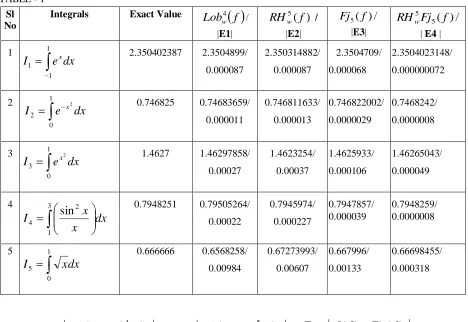
TABLE - 1 Sl No
Integrals Exact Value
Lob
f
w
4
/
|E1|
)
(
5
f
RH
w /|E2|
/
)
(
5
f
Fj
|E3|
/
)
(
5 5
f
Fj
RH
w | E4 |1
11 1
e
dx
I
x 2.350402387 2.3504899/0.000087
2.350314882/
0.000087
2.3504709/
0.000068
2.3504023148/
0.000000072
2
10 2
2
dx
e
I
x 0.746825 0.74683659/0.000011
0.746811633/
0.000013
0.746822002/
0.0000029
0.7468242/
0.0000008
3
10 3
2
dx
e
I
x 1.4627 1.46297858/0.00027
1.4623254/
0.00037
1.4625933/
0.000106
1.46265043/
0.000049
4
31 2
4
sin
dx
x
x
I
0.7948251 0.79505264/
0.00022
0.7945974/
0.000227
0.7947857/ 0.000039
0.7948259/ 0.0000008
5
10 5
x
dx
I
0.666666 0.6568258/
0.00984
0.67273993/
0.00607
0.667996/
0.00133
0.66698455/
0.000318
Where
E
1
I
(
f
)
Lob
w4(
f
)
,(
)
(
)
5
2
I
f
RH
f
E
w ,E
3
I
(
f
)
Fj
5(
f
)
,)
(
)
(
5 54
I
f
RH
Fj
f
E
w are errors of various rules.Using the results of the table and the notations for the errors of different methods given above the table , four bar graphs for the errors of the mixed quadrature rule and its constituent rules have been constructed in figures
A,B,C and D correspond to
11 1
e
dx
I
x ,
1
0 2
2
dx
e
I
x ,
1
0 3
2
dx
e
I
x and
3
1 2
4
)
sin
(
dx
x
x
I
respectively.
In the four graphs ,the error names of the mixed quadrature rule and its constituent rules have been embedded along X-axis and the respective values of the errors depicting heights of the bars are given along Y-axis.The graphical representation of these errors is given above in figures:A,B,C,D.From the above four graphs the unit in Y-axis is :
6 5
4 3
2 1
10
log
6
,
10
log
5
,
10
log
4
,
10
log
3
,
10
log
2
,
10
log
1
.Thus from the graphs , we conclude that larger the height of the bar the smaller is the error. Here we derived most significant result that our mixed rule is more accurate than its constituent rules.
6 Adaptive quadrature algorithm A simple Adaptive Strategy
Given a real integrable function
f
an interval[
a
,
b
]
and a prescribed tolerance
, it is desired to compute anapproximation
P
to the integralI
f
x
dx
b
a
(
)
, So thatP
I
.This can be done following adaptiveintegration schemes developed in papers [4-7,9,12,13]. In adaptive integration, the points at which the integrand is evaluated are chosen in a way that depends on the nature of the integrand. The basic principle of adaptive quadrature routines is discussed in the following manner.
If
c
is any point betweena
andb
then
bc c
a b
a
dx
x
f
dx
x
f
dx
x
f
The idea is that if we can approximate each of the two integrals on the right to within a specified tolerance, then the sum gives us the desired result. If not we can recursively apply the adaptive property to each of the intervals
]
,
[
a
c
and[
c
,
b
]
. Adaptive subdivision of course has geometrical appeal. It seems intuitive that points should be concentrated in regions where the integrand is badly behaved. The whole interval rules can take no direct account of this.In this paper we design an algorithm for numerical computation of integrals in the adaptive quadrature routines involving mixed rules. The literature of the mixed quadrature rule [9,14-16] involves construction of a symmetric quadrature rule of higher precision as a linear/convex combination of two other rules of equal lower precision.
Algorithm for adaptive quadrature routines:
The input to this schemes is
a
,
b
,
,
n
,
f
,
the output
b
a
dx
x
f
I
(
)
with the error hopefully less than
,
n
is the number of intervals initially chosen. A Simple adaptive strategy is out lined in the following step algorithm.Step - 1 :An approximation
I
1 to
b
a
dx
x
f
I
(
)
is computed.Where
2
b
a
c
and then
c
a
dx
x
f
I
2(
)
and
bc
dx
x
f
I
3(
)
are computed.Step - 3 :
I
2
I
3 is computed with toI
1 estimate the error inI
2
I
3.
Step - 4 :If | estimated error |
2
(termination-criterion), thenI
2
I
3 is accepted as an approximationto
b
a
dx
x
f
I
(
)
. Otherwise the same procedure is applied to[
a
,
c
]
and[
c
,
b
]
allowing each piece a toleranceof
2
.TABLE - 2 Sl
No
Integrals Exact Value
Lob
f
w
4
No. of. step |Error|
)
(
5
f
RH
wNo. of. step |Error|
)
(
5
f
Fj
No .of. step|Error|
)
(
5 5
f
Fj
RH
wNo .of. step |Error|
Prescribed tolerance
1
11 1
e
dx
I
x 2.350402387 2.35040241103
0.000000031
2.350402351
03
0.000000028
2.350402383
03
0.000000003
2.3504023896
01
0.000000009
0.00001
2
10 2
2
dx
e
I
x 0.746825 0.74682413303
0.00000086
0.746824128
03
0.0000008
0.746824124
01
0.0000008
0.746824133
01
0.0000008
0.00001
3
10 3
2
dx
e
I
x 1.4627 1.4626517605
0.000048
1.46265172
05
0.000048
1.46265172
03
0.000048
1.462651739
01
0.000048
0.00001
4
31 2
4
sin
dx
x
x
I
0.7948251 0.79482521
03
0.0000002
0.79482514
03
0.00000014
0.79482517
03
0.00000017
0.794825183
01
0.00000018
0.00001
5
dx
x
I
1
0 5
0.666666 0.6666642
15
0.000017
0.6666681
15
0.0000021
0.6666692
11
0.0000032
0.6666684
09
0.0000024
0.00001
Adaptive quadrature routines essentially consist of applying the mixed rule
RH
w5Fj
5(
f
)
and its constituents rules)
(
4
f
Lob
w , 5(
)
f
RH
w andFj
5(
f
)
are to each of the sub intervals covering until the termination criterion isfurther sub divided and the entire process repeated. The result obtained by a shorter program in standard CPP which should be more transportable and efficient.
7 Observation
In whole interval routine from the table-1 as well as from the bar graph it is observed that the absolute error corresponding to the mixed rule 5
(
)
5
f
Fj
RH
w is lesser than those corresponding to its constituent rules)
(
),
(
),
(
55 4
f
Fj
f
RH
f
Lob
w w are compared and mixed rule is better than its constituents rules, when the testintegrals are evaluated .However when these rules are used in adaptive mode, table-2 depict that the mixed quadrature rule using anti-Gaussian rule give very good result and less number of steps than its constituent rules when tested on a number of integrals.
8. Conclusion :
After observation one can smartly draw conclusion over the efficiency of the rule formed in this paper as follows: (1) The mixed
RH
w5Fj
5(
f
)
rule is more efficient than its constituent rulesLob
w5(
f
),
RH
w5(
f
),
Fj
5(
f
)
and previously developed mixed rules.(2) In this paper we have concentrated mainly on computation of definite integrals in the adaptive quadrature routines involving mixed quadrature rule. We observed that mixed quadrature rule so formed can be very well used for evaluating real definite integrals than its constituent rules in the adaptive quadrature routines.
Acknowledgement:
The research work has been supported by the Department of Science and Technology, Govt. of India under INSPIRE Fellowship and my code no is IF10203. I also thankful to Director and Professor of Institute of Mathematics and Application, BBSR, Odisha , India (my place of research),who guide me and provide good research facilities.
REFERENCES :
[1] Dirk P. Laurie, Anti-Gaussian quadrature formulas, mathematics of computation,65(1996)pp. 739-749.
[2] Dirk P. Laurie, Computation of Gauss-type quadrature formulas, Journal of Computational and Applied mathematics of computation,127(2001)pp. 201-217.
[3] Dirk P. Laurie, Stopping functionals for Gaussian quadrature formulas, Journal of Computational and Applied mathematics ,127(2001)pp. 153-171.
[4] Dirk P. Laurie, Sharper error estimates in adaptive quadrature, BIT,(1983)CMP,23:258-261,MR84e:65027.
[5] Dirk P. Laurie, Practical error estimation in numerical integration, Journal of Computational and Applied mathematics ,(1985)CMP,17:14,12 and 13:258-261.
[6] J. Berntsen, Practical error estimation in adaptive multidimensional quadrature routines, Journal of Computational and Applied mathematics,25(1989),327-340,North-Holland.
[7] J. Berntsen, T.O. Espelid and T.Sorevik.,On the subdivision strategy in adaptive quadrature algorithms, Journal of Computational and Applied mathematics ,35(1991),119-132.
[8] S. Conte. and C.D. Boor., Elementary numerical analysis , Mc-Graw Hill, (1980).
[9] C.W.Clenshaw and A.R.Curties, A method 700 numerical integration on an automatic computer,Numer.Math,2 ,(1960),MR22:8659,197 -205.
[10] F. Lether ., On Birkhoff-Young quadrature of analytic function, J. Comp. Applied Math.2, 2(1976) , pp.81-84 . [11] Atkinson Kendall E.,An introduction to numerical analysis , 2nd edition ,John Wiley and Sons,Inc, (1989).
[12] A.C.Genz and A.A.Malik(*).,Remark on algorithm 006: An adaptive algorithm numerical integration over an N -dimensional rectangular region, Journal of Computational and Applied mathematics , (1980),volume 6,No 4.
[13] P.V. Dooren and L.de. Ridder.,An adaptive algorithm numerical integration over an n-dimensional cube, Journal of Computational and Applied mathematics , (1976),volume 2,No 3.
[14] B.P. Acharya and R.N. Das., Compound Birkhoff –Young rule for numerical integration of analytic functions.Int.J.math.Educ.Sci.Technol 14(1983),pp.91-101.
[15] R.N. Das and G. Pradhan ., A mixed quadrature rule for approximate value of real definite Integrals, Int. J. Edu. Sci. Technol, 27 (1996), pp. 279 - 283.
[16] R.N. Das and G. Pradhan .,A mixed quadrature Rule for Numerical integration of analytic functions, Bull. Cal. Math. Soc., 89 (1997) ,pp.37 - 42.
[17] A. Begumisa and I. Robinson., Suboptional Kronrod extension formulas for Numerical quadrature , math, MR92a(1991),pp.808-818. [18] Walter. Gautschi., Gauss-Kronrod quadrature –a survey, In G.V. Milovanovic. Editor, Numerical Methods and Approximation Theory III,