Surface water flow in landscape models:
1. Everglades case study
Alexey A. Voinov *, H. Carl Fitz, Robert Costanza
Institute for Ecological Economics(IEE),Uni6ersity of Maryland,P.O.Box38,Solomons,MD20688-0038,USA
Accepted 20 November 1997
Abstract
Many landscape models require extensive computational effort using a large array of grid cells that represent the landscape. The number of spatial cells may be in the thousands and millions, while the ecological component run in each of the cells to account for landscape dynamics is often process based and fairly complex. To compensate for the increased computational complexity of the model there is a tendency to simplify the hydrologic component that fluxes material horizontally across the landscape. Instead of full scale hydrologic models based on stable implicit schemes, computationally simpler explicit algorithms are incorporated and run with quite large time steps. As a result some fairly inadequate behavior may be observed, especially when the temporal and spatial steps are modified without due care. We illustrate these problems with a series of runs performed using the Everglades Landscape Model (Southern Florida, USA), that covers an area of more than 10000 km2. Several algorithms for hydrologic fluxing are compared
in terms of their computational complexity and stability. We argue that a compromise can be drawn by supplement-ing the explicit modelsupplement-ing scheme with a series of additional checks and conditions that provide for model stability, and with some empirical assumptions that allow the model to operate over a sufficiently large range of temporal and spatial scales. © 1998 Elsevier Science B.V. All rights reserved.
Keywords: Landscape spatial modeling; Hydrology; Temporal and spatial resolution; Manning’s equation; Overland flow
1. Introduction
In landscape models hydrology plays an impor-tant driving role. Surface and subsurface flows of
water serve as a major transport mechanism, both delivering the essential elements to the biota and removing the constituents in excess. The impor-tance of hydrologic transport has been long rec-ognized and considerable effort has been put into creating adequate models for various landscapes (Beven and Kirkby, 1979; Beasley and Huggins, 1980; Grayson et al., 1992).
* Corresponding author. Tel:+1 410 3267207; fax:+1 410 3267354; e-mail: [email protected]
A.A.Voino6et al./Ecological Modelling108 (1998) 131 – 144 132
Nevertheless there are no off-the-shelf univer-sal models that can be easily adapted for a wide range of applications. Significant effort is needed to tune existing models to the specifics of the landscape and the goals of the study. This is because hydrologic modeling as a part of larger landscape modeling imparts certain conditions on the methods used. Being part of a more com-plicated modeling structure, the hydrologic mod-ule is required to be simple enough to run within the framework of the integrated physico-ecological model. As a result some hydrologic details need be sacrificed to make the whole task more feasible, and these details may differ from one application to another, depending upon the sizes of the study area, the physical characteris-tics of the slope and surface, and the goals and priorities of the modeling effort.
Another trade-off specific to landscape scale models is the coarser spatial and temporal reso-lution that they usually employ in contrast to the classic hydrologic methods that were primar-ily developed for small scale, well sampled, repli-cated and controlled systems. While most of the methods and equations in classic hydrology have been developed for sizes on the order of meters and times on the order of hours and less, this is hardly the resolution that landscape models can afford. As a result discrete approximations of the essentially continuous hydrologic processes become a source of potential problems. In place of a continuous movement of water and con-stituents over the area we need to deal with essentially discrete motions, when large volumes of material are moved over large distances on relatively rare occasions.
Among the simplified approaches to surface water fluxing, the prevailing ones are based on the kinematic wave approximation of the St. Venant’s equations (Beven and Wood, 1993). These are solved numerically, with the implicit scheme bearing all the advantages of being sta-ble for any chosen time and space intervals (Greco and Panattoni, 1977). This approach is most common in modeling linear flood routing in rivers and canals. However in models of 2-di-mensional overland flow the implicit scheme is
usually substituted by a computationally simpler explicit one. For example, this approach was adopted in the SHE model (Abbott et al., 1986), where channel flow was modeled by an implicit scheme, but the overland flow scheme used an explicit procedure. Because the solution of the implicit method is essentially based on the boundary conditions, the advantages of the ex-plicit approach become especially obvious when we need to consider a region that has complex boundaries or if it is further subdivided into subregions by some impermeable borders (levees) or if it has other kinds of disturbances like a network of canals, that is not attached to the underlying elevation data.
On the other hand, with the obvious advan-tage of computational simplicity, when running the explicit scheme we should realize that there is always a risk of destabilizing the model, espe-cially if we modify its temporal or spatial resolu-tion. This was the situation we encountered in modeling hydrologic fluxes within the framework of the Everglades Landscape Model (ELM). The problem was further complicated by the rela-tively large size of the area to be considered. While ANSWERS (Beasley and Huggins, 1980) has been recommended for watershed sizes less than 100 km2, and TOPMODEL was tested for
catchments of up to 10 km2 (Beven et al., 1984),
in our case we were looking at an area orders of magnitude larger than that, roughly 10000 km2.
Moreover the hydrologic component was to be embedded in a fairly detailed process-based sim-ulation model of terrestrial and aquatic biota. This necessarily implied certain restrictions and conditions on the methods to be used.
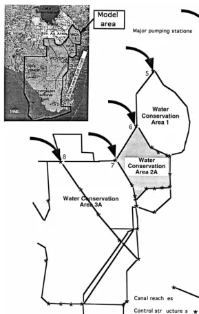
Fig. 1. ELM area. Expanded is the area with the canals, where most of the water fluxing occurs.
2. Hydrologic module in the Everglades landscape model
The Everglades Landscape Model (ELM) is designed to simulate the landscape scale vegeta-tion response to simulated hydrology, water quality and fire. The ELM has a fine scale grid
that divides the landscape into 10000 1 km2 cells
A.A.Voino6et al./Ecological Modelling108 (1998) 131 – 144 134
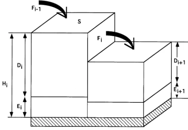
Fig. 2. Geometry of a 1-dimensional flow. Horizontal fluxing is driven by the head difference. The water head is determined as a sum of elevationEiand the surface waterDi.
Overland sheet flow and groundwater move-ments are some of the principal fluxes of water across the landscape and they regulate the plant and animal community structure. A large network of canals, levees, and associated flow control structures are used for water management in the region. The canals are a significant water trans-port mechanism in the Everglades, moving large quantities of water further and more rapidly than the comparatively slow overland flow. The inter-action of canals with overland sheet flow is de-scribed elsewhere (Voinov et al., submitted).
Within each raster cell the unit model simulates a variety of hydrologic processes and parameters (Fitz et al., 1996), including the following:
1. Transpiration associated with plant growth, physiology and relative humidity.
2. Evaporation using pan evaporation estimates and pan coefficients.
3. Rainfall based on precipitation data interpo-lated over nine stations.
4. Seepage of water from that stored above the sediment/soil surface into that stored in sedi-ment pore space (either in unsaturated or satu-rated storage).
5. Roughness coefficient that depends on
dy-namic simulation of plant biomass, numeric density, and plant morphology.
After the water head in each raster cell is modified due to vertical fluxes, the surface water movement between the raster cells (and associated transport of constituents) is calculated. The sim-plest way to do this is to look at the flow between two adjacent cells I andI+1 as flow in an open channel and use the so called slope – area method (Boyer, 1964), which is a kinematic wave approxi-mation of St. Venant’s momentum equation. The flux (m3/d) in this case is described by the
empiri-cal Manning’s equation for overland flow:
F=A·R2/3·G1/2/M,
where A is the cross-sectional area of water flux,
Ris the hydraulic radius andGis the slope of the energy gradient. In discrete terms used in the model (Fig. 2), assuming that the cells are squares of the same areaS, and that the energy gradient is determined by the head difference over the grid size, the equation can be rewritten as:
F=sgn(Hi−Hi+1) ·Hi−Hi+1·D5/3·4S/M
whereF is the flux of water (m3/d) between cells,
Hi and Hi+1 are the hydraulic heads (m) of the
cells, which result from adding the surface water depth (Di) to the cell elevation (Ei);S is the area
(m2) of the surface water in the cell (assuming
that both cells have the same area); D=(Di+ Di+1)/2 is the average depth of the surface water
(m) in the two interacting cells, and M=(Mi+ Mi+1)/2 is the average Manning’s coefficient of
surface roughness. The algorithm based on this flow calculation we will call ‘proper Manning’s algorithm’ and refer to it as Method N1.
The Manning’s roughness coefficient in a cell is a function of the sediment type and the interac-tion of the vegetainterac-tion height/density and water depth:
M=Mmax−(Mmax−Mmin) · (2(1−D/Hm)−1 (2)
The Mmin roughness is the minimum Man-ning’s coefficient for a vegetation-free cell, the
Mmax is the maximum roughness associated with
the (dynamic) vegetation density in the cell, and
Hmis the (dynamic) height of the macrophytes in
the cell. This function returns a roughness coeffi-cient whose value ranges from a vegetation-free minimum to a maximum at the point of full plant immersion (Petryk et al., 1975). As water depth increases over that of the macrophyte height, the roughness decreases to an asymptote at the base-line sediment roughness (Nalluri and Judy, 1989).
St. Venant’s continuity equation:
(A (t= −
(F (x
in its discrete form provides for a means to link a cell to the neighboring ones:
Di(t+Dt)=Di(t)+(Fi−1(t)−Fi(t))Dt/S. (3)
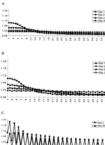
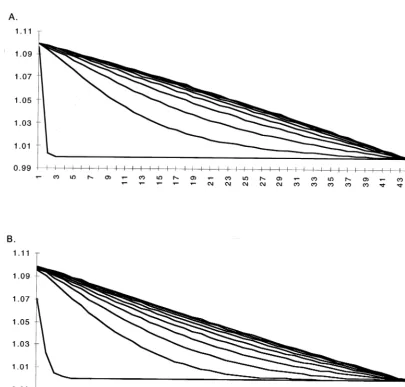
This equation works well as long as the outflux from the cell does not exceed the sum of the influxes and the available water volume in a cell. Moreover it would be quite unrealistic if because of the fluxing, the water head in the recipient cell exceeds the water head in the donor cell. These events obviously will become more likely as the time step Dt grows. We may illustrate this on a series of test runs on a cross-section of cells. We assume an initially homogeneous distribution of
water over the cells except for a 1 m higher head in the first cell. With Dt=0.005 the resulting distribution is fairly smooth, however already with this small time step we may observe persist-ing slight oscillations, where the water levels out in the cells (Fig. 3A). As the time step is in-creased to Dt=0.01 (Fig. 3B) and further to
Dt=0.05 (Fig. 3C) the oscillations increase and their amplitude tends to increase with time, even-tually destabilizing the model.
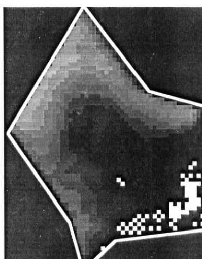
In the 2-dimensional case this instability results in, what we call, a ‘checker-board’ pattern (Fig. 4), the situation described by Chow et al. (1988) as an accumulation or piling up of water, when the time step is larger than the time needed for a wave to travel the distance of the cell width. This is the Courant condition which is necessary (but not sufficient) for stability of explicit schemes:
Dx/Dt]F/S,
where, as above, F is the flux of water (m3/d),
and Sis the area (m2) of the surface water in the
cell. This condition implies that the most natural way to make the model stable would be to reduce the time step, when we need to run the model at a finer spatial resolution. However this is in conflict with our initial desire to run the model at larger time steps to decrease the amount of CPU time needed, even at the expense of some preci-sion.
To mitigate this problem another condition is added to the model, which effectively slows down the flux rate, preventing further water fluxing once the heads in two adjacent cells are balanced. Eq. (1) is replaced by:
F=sgn(Hi−Hi+1) · min
!
S·Hi−Hi+12 ,Hi−Hi+1·D
5/3·4S·Dt
M
"
/Dt(4)
A.A.Voino6et al./Ecological Modelling108 (1998) 131 – 144 136
Fig. 3. Distribution of water over the cells in time with different time steps in the model. A.Dt=0.005; B.Dt=0.01; C.Dt=0.05 day.
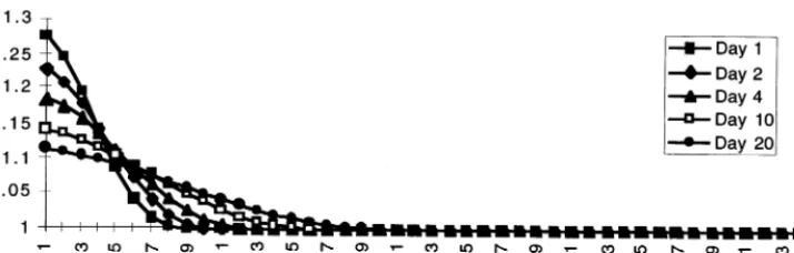
With this restriction we can increase the time step quite significantly while still keeping the model stable. In Fig. 5 the propagation is calcu-lated with a time step of Dt=0.5, which is ten
Fig. 4. ‘Flip-flop’ checkerboard patterns observed in model results when the time step is large. The checkerboard pattern appears first in the areas with the lowest water heads (as in this picture), the oscillations do not tend to dampen out, on the contrary they tend to grow eventually destabilizing the model.
fails to reach equilibrium, when the head differ-ence between cells becomes small. At the same time Method N2 is hardly adequate for rapid water transport, but it certainly performs better than Method N1 when flow dynamics are slow and head differences are small. If we modify the test scenario so that there is a constant source that maintains a certain water head on the left hand side and an open boundary, that allows excess water to flow out — on the right hand side, we may observe (Fig. 6) that both methods per-form in almost the same way. They are identical once the steady state distribution is reached. The only obvious distinction in these model runs is that Method N1 operates with a time step ten times smaller than Method N2. Actually Method N2 can run even at larger time steps and produce results similar to Method N2 as long as the perturbation from the steady state is small.
Once the interaction between two cells is deter-mined, we need to figure out how all the cells can be linked spatially over the landscape. This imme-diately causes some controversy, because from the 1-dimensional channel flow assumption we need to expand to the 2-dimensional water flow and there may be a variety of options to generalize the pairwise interaction described above over the mul-titude of cells in the landscape.
The flow separation in the north – south (NS) and east – west (EW) directions is not of a major concern, because in ELM the elevation gradient is very small and fairly uniform, with only 5 m gain over the 108 km×184 km covered by the study area. Therefore the slope can be considered equal water across the cells becomes asymptotic, slowly
tending to the equilibrium, that was achieved in the previous method in a matter of a few days.
Comparing Method N1 and Method N2, we may observe that the first one is certainly more realistic when large quantities of water are to be moved rapidly across the landscape. However it
A.A.Voino6et al./Ecological Modelling108 (1998) 131 – 144 138
Fig. 6. Comparison of model runs over days 1 through 10 with Method N1 (A.) and Method N2 (B.) The flow scenario in this case is defined by a constant head on the left hand end and an open boundary on the right hand end.
in all directions, and there is no need to bother with flow separation, since in any case it is more likely to be defined by microelevation properties, ignored in the model, than by the elevation gradients.
Among the possible patterns of interaction be-tween the cells, probably the simplest one assumes that each cell is interacting with its four immedi-ate neighbors, and that the flows in the NS and EW directions are independent and simultaneous. This approach was applied to the whole model area (Fig. 1), which was scanned twice: first there
was a loop to calculate all the potential fluxes
VFi,j in the NS and HFi,j in the EW directions,
based on the existing water heads, surface water depths and vegetation in the cells; next during the second loop the water depthsDijwere recalculated
applying Eq. (3) modified for four fluxes. This approach, though requiring extra memory to store the two intermediate flow arrays, has the advan-tage of being independent of the order in which the cells are scanned.
scheme. In fact, if each flow is calculated indepen-dently, with no account of the head change due to the flux that has been already computed, one can easily drain the cell below zero. This is especially likely to occur if we keep the time steps suffi-ciently large. To avoid this a series of additional checks are implemented when calculating the fluxes for each cell. First the four potential fluxes
HFi−1,j, HFij, VFi,j−1, and VFij are calculated.
The variable ‘out’ is calculated as a sum of all potential flows out of the cell and the variable ‘in’ is the sum of all potential flows into the cell. Next the potential new headD=Dij+(in−out)Dt/Sis
compared to the minimal head in the interacting adjacent four cells. If it is lower:
D−min(Di−1,j;Di+1,j;Di,j−1;Di,j+1)B0 (5)
it means that at some point, if the potential fluxes were to be realized, water would have to move against the gradient, further draining the donor cell. In order to avoid this unrealistic and destabi-lizing situation, all the fluxes out of the cell, that make the variable ‘out’ above, are proportionally decreased so that condition Eq. (5) would no longer hold.
At the 1 km2 resolution of the full Everglades
model, we did not observe significant head differ-ences and Method N2 could be used as a valid approximation. After some adjustments in the rate parameters the method produced fairly rea-sonable results even at sufficiently large time steps (Dt=0.5 day). It is impossible to present these results within the format of this publication, since the output is generated as color animations. We therefore refer the reader to our WWW page at http://kabir.cbl.cees.edu/Glades/ELM.html, were results of various model runs are presented and comparison to existing stage data is provided.
It would be certainly wrong to recommend Method N2 for general use, since it’s performance is not adequate when flow rates are high and head differences are significant. In that case we should either consider a combination of Methods N1 and 2, when the first method with a small time step is run until the water heads sufficiently equilibrate (DB0.1 m), and then Method N2 kicks in to handle the quasi-equilibrium conditions at much larger time steps, or use an alternative algorithm, discussed below as Method N3.
3. The CALM case-study
It is still quite a large job to calibrate the whole landscape model running it over the almost 10000 cells of the full ELM model. A one year run takes almost 2.5 h on a Sparc 10 Sun workstation. Therefore it was decided to cut out a relatively small portion of the ELM area to perform a more vigorous test of the model. Water Conservation Area 2A (shaded area in Fig. 1) was chosen because of the additional data available for that region, primarily on the elevations and habitat types (Jensen et al., 1995). Since the habitat data had a better resolution than the 1 km2 used in
ELM, a finer grid of 0.25 km2 was developed for
this subregion. This also served the goal of testing some of the scaling issues. This truncated ELM model was called CALM (Conservation Area Landscape Model).
The initial plan was to run the model un-changed just switching to the other set of data files. Running the straight Manning’s method would require at least a four times smaller time step to compensate for the finer spatial resolution in CALM. But this would take away almost all the gain we got by diminishing the model area. Therefore we were primarily looking at the equili-brating method.
The problem was that because Eq. (4) effec-tively slows down the water fluxing, we were not getting the water redistributed fast enough. This turned out to be crucial in our case, where due to the artificially controlled flow through the system of canals and structures, on certain occasions the landscape was receiving quite significant amounts of water, that needed to be quickly propagated throughout the model area. When divided by the 1 km2in the full ELM resolution, the water heads
quanti-A.A.Voino6et al./Ecological Modelling108 (1998) 131 – 144 140
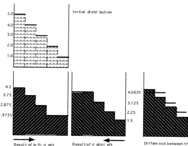
Fig. 7. Difference generated by the two sequencing algorithms. When running through the cells from left to right, and equilibrating water levels in them, we end up with a distribution different from the one we get, if cells are treated in reverse order.
ties received from Water Conservation Area 1 through a series of structures. Unless the water was moved spatially quickly enough very signifi-cant water heads could build up. The equilibrium condition Eq. (4) worked well for purposes of stabilizing the model, but it also prevented fast propagation of water.
As an alternative to the two step surface water calculation applied above, we now allowed water to be fluxed immediately as the flux was lated according to Eq. (4). Instead of first calcu-lating all the potential fluxes between the cells, storing the results and only then, in a separate loop over all the cells, actually recalculating the water heads, in this new scheme as soon as the flux F was defined, the water heads in the corre-sponding cells were recalculated:
Di(t+Dt)=Di(t)−Fi(t) ·Dt/S
Di+1(t+Dt)=Di+1(t)+Fi(t) ·Dt/S
To do that we also had to consider the NS and EW fluxing separately. That is, first all the land-scape cells were updated for the fluxes in the EW direction, and then over a separate loop all the NS fluxes were calculated and water heads were updated once again.
In this way, if water rose in ith cell, then the water head in the (i+1)st cell was updated and also rose prior to calculating the flux Fi+1 to the
cell (i+2), therefore increasing this flux, and so on. This allowed for faster water transfer, but also made the process dependent upon the order of cell sequencing. In fact, if we were moving in the opposite direction through the cells, we would be getting fairly different results (Fig. 7).
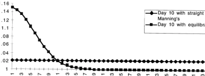
Fig. 8. Comparison of the water distribution generated by the straight Manning’s algorithm withDt=0.001 and the equilibrating algorithm withDt=0.5. By day 10 there is still a significant difference in the way the two algorithms accommodate a 1 m pulse of water. This difference is significantly smaller when the variations of water are small (B0.5 m).
the westernmost cell and going back to the east. Similarly first the NS loop was run from north to south and then back from south to north. This doubled the number of computations needed, but made the procedure symmetric with respect to the order that the cells were considered.
In this way we got a better control over the fluxes in the landscape and could distribute water somewhat more rapidly over the area. Another advantage of this method was that condition Eq. (5) was no longer needed and therefore there was no longer any potential for mass disbalance in the system. However, because of the condition Eq. (4) still in place, occasionally when pulses of pumping are especially high, we could develop unrealisti-cally high water heads. The difference with the proper Manning’s method (Method N1) run at
Dt=0.001 is still quite substantial (Fig. 8), espe-cially when the head difference is large. The equi-librating algorithm (Method N2) is quite efficient in dealing with the small variation of water heads, when there are no significant pulses and associ-ated rises in water heads. In this case the results turn out to be quite close to the base line proper Manning’s simulations, and the gain in model efficiency is quite substantial because similar re-sults can be generated with 500 times larger time steps.
The method was further modified to accommo-date the large pulses, that we had to deal with in CALM. Once the Manning flux in Eq. (5) was so large that it tended to disequilibrate the two
adja-cent cells, instead of curtailing the flux and limit-ing it to the amount that would equilibrate the two adjacent cells as in Eq. (4), it was assumed that water could be fluxed over more than one cell in one time step. In this way, over one time step, the high water head can be redistributed across as many cells in the landscape as needed to accom-modate the excess of water, as long as the heads in those cells are initially lower than the equi-librium thus attained. The propagation of water stops once a cell with a higher water head, or the boundary is reached. This assumption seems to be quite appropriate since over a large time step water in fact will probably travel further than over one adjacent cell.
To maintain some control over the process an additional model parameter is introduced. This parameterVis to be specified as the allowed head difference between any two cells. It is also as-sumed that if the head difference between two cells is initially BV, then this condition is not applied and water is fluxed across these cells, while it is in excess.
Thus, for theith donor cell we first identify the number of cells N to interact with as recipients. Let TN=SHi+j, j=0,…,N, and Fi be the
Man-ning’s flux calculated according to Eq. (1). Then
Nis incremented whileHi+N5TN−1/N−V·N/2
A.A.Voino6et al./Ecological Modelling108 (1998) 131 – 144 142
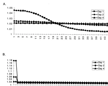
Fig. 9. Comparison of the straight Manning’s algorithm (A) with the distributing one (B) withV=0.5. Even though the transfer process is different, by day 4 both methods equilibrate to the same distribution pattern.
25min(Fi, (Hi−Hi+1)) (to ensure that there is
still water to flux according to the calculated Manning’s flow and that this flow is not larger than the head difference between theith cell and its next neighbor).
For these N cells the water heads are then recalculated:
Hi+j=TN/N+V· (N−2 ·j−1)/2,
j=0,…,N.
We useVessentially as a calibration parameter to achieve distribution patterns close to those generated by the proper Manning’s method run with very small time steps on a trial basis. The smaller the allowed head difference V, the smoother the propagation of water, the more water is fluxed in one iteration after a pulse has occurred and the slower the water equilibrates afterwards. WithV=0 the equilibrium may be attained over
one step. In contrast, with sufficiently largeVthe attained distributions are almost step-wise, but eventually the equilibrium is reached faster, be-cause more water is distributed over the cells that are not limited by the Vcondition.
As a result even under conditions of extremely high water deliveries into the system, the model quickly converged to the same water head values as we were to get in the straight Manning’s method with very small time steps (Fig. 9). The transfer stages do look somewhat different, but in a matter of several days we were getting almost the same distribution. We have tested this method for sev-eral scenarios of pumping and even for time steps as large as several days it produced fairly stable results, which were within a 10% error compared with the available observed data. Once again we refer the reader to our WWW page at http://
Fig. 10. Distribution of water in the generalized Manning’s method withb=1.5 andDt=0.01. Even with the larger time step the pattern is smooth (compare to Fig. 3B that had the same time step), but the rate of propagation has decreased.
4. Conclusion
The methods suggested can be considered as an empirical approach to surface water routing. It is certainly very much based on some empirical as-sumptions and common sense. However we should remember that the Manning’s equation is also empirical and in fact in many applications Eq. (1) is generalized to
F=a·Db (6)
wherea and b are offered as empirical constants (Beven and Wood, 1993; Novotny and Olem, 1994 ). Actually this means that in surface hydrology, especially in models of this scale and resolution, there is still quite a lot of empiricism to allow the kind of manipulations that we have applied, espe-cially if the results turn out to be adequate.
The major problem with the proper Manning’s equation is that b=1/2. With such b and small values of D (D1) the change in the flux rate, calculated in Eq. (1), becomes relatively much larger than the variations inD. As a result, as we saw in Fig. 3A, even with very small time steps there are certain instabilities in the region of small water head differences. In those areas where the really signifi-cant water fluxes occur (left hand side in Fig. 3), we see no instabilities even with larger time steps. But it is the area of quasi-equilibrium that causes most of the trouble and requires smaller time steps. It is interesting to note that with b=1 or 1.5 we get a much smoother distribution at significantly larger time steps (Fig. 10), which actually very much resembles the picture observed in the
cell-equilibrat-ing algorithm (Method N2) (see Fig. 5). Varycell-equilibrat-ingb we can choose between faster distribution over the landscape and more stability at larger time steps. The b=1/2 easily justified by Newtonian me-chanics, seems to contradict with the kinematic wave approximation for the St. Venant’s equation. Neglecting the gravity wave terms in this equation, makes it nearly impossible to reach equilibrium, eventually resulting in the ‘flip-flop’ dynamics, that can continue indefinitely with no trend towards stabilization. On the contrary it has a possible destabilizing effect.
It has been observed that Manning’s equation can be easily misused. Kadlec (1990) argues that mod-eling sheet flow in wetlands is one such case, where the flow is not turbulent enough to use the Man-ning’s equation properly, though it is not quite laminar as well. He suggests to useb=1 in those cases when we find the flow to be more laminar than turbulent. Interestingly, we have arrived at quite similar conclusions based on purely theoretical observations about stability of various modeling methods.
A.A.Voino6et al./Ecological Modelling108 (1998) 131 – 144 144
in model efficiency in terms of the CPU time required. In this case we have to rely more on the comparison of the model output with the data available, and be ready to switch from the more process based description to a more empirical one as in Eq. (6). As can be seen on the Web page, the results that we have been obtaining for the Ever-glades seem to match fairly well with the experimen-tal data available on water heads. This speaks in favor of the methods applied.
Certainly by choosing this approach, by diverg-ing from the process-based paradigm and by allow-ing more parameter and formulae calibration, we decrease the generality of the model, thus requiring additional testing and calibration when switching to other scales or areas. The question is what is a truly process-based model as against an empirical, regression one. In any process-based model there is a certain level of abstraction at which we actually utilize certain empirical generalizations, rather than true process description. For example, there is hardly an adequate detailed biophysical molecular description of the photosynthesis process to be found among the models of vegetation growth, instead some variations of Michaelis – Menten ki-netics are applied, which are already empirical generalizations of the process. Nevertheless these models claim to be process-based. As we go to larger systems, such as landscapes, we will need to employ even more generalized formalizations, as was done above for modeling hydrology in the Everglades.
Acknowledgements
This research has been conducted under a con-tract with the South Florida Water Management District.
References
Abbott, M.B., Bathurst, J.C., Cunge, J.A., O’Connell, P.E., Rasmussen, J., 1986. An introduction to the European
Hydrological System — Systeme Hydrologique Europeen. SHE 2: Structure of a physically-based, distributed mod-elling system. J. Hydrol. 87, 61 – 77.
Beasley, D.B., Huggins, L.F., 1980. ANSWERS (Areal Non-point Source Watershed Environment Response SImula-tion), User’s Manual. Purdue University, West Lafayette. Beven, K., Wood, E.F., 1993. Flow routing and the hydro-logical response of channel networks. In: Beven, K., Kirkby, M.J. (Eds.), Channel Network Hydrology. John Wiley, Chichester.
Beven, K.J., Kirkby, M.J., Schofield, N., Tagg, A.F., 1984. Testing a physically-based flood forecasting model (TOP-MODEL) for three UK catchments. J. Hyrol. 69, 119 – 143.
Beven, K.J., Kirkby, M.J., 1979. A physically-based, variable contributing area model of basin hydrology. Hydrol. Sci. Bull. 24 (1), 43 – 69.
Boyer, M.C., 1964. Stream flow Measurements. In: Chow, V.T. (Eds.), Handbook of Applied Hydrology. McGraw-Hill, New York, pp. 15.1 – 15.42.
Chow, V.T., Maidment, D.R., Mays, L.W., 1988. Applied hydrology. McGraw-Hill, New York.
Fitz, H.C., DeBellevue, E., Costanza, R., Boumans, R., Maxwell, T., Wainger, L., Sklar, F., 1996. Development of a general ecosystem model for a range of scales and ecosystems. Ecol. Model. 88 (1/3), 263 – 295.
Grayson, R.B., Moore, I.D., et al., 1992. Physically based hydrologic modeling: 1. A Terrain-based model for inves-tigative purposes. Water Resour. Res. 28 (10), 2639 – 2658.
Greco, F., Panattoni, L., 1977. Numerical solution methods of the St Venant equations. In: Ciriani, T.A., Maione, U., Wallis, J.R. (Eds.), Mathematical Models for Surface Water Hydrology. Wiley, London, New York, Sydney, Toronto, pp. 181 – 194.
Jensen, J.R., Rutchey, K., Koch, M.S., Narumalani, S., 1995. Inland wetland change detection in the Everglades water conservation area 2A using a time series of nor-malized remotely sensed data. Photogramm. Eng. Remote Sens. 61 (2), 199 – 209.
Kadlec, R., 1990. Overland flow in wetlands: vegetation re-sistance. J. Hydraul. Eng. 116 (5), 691 – 706.
Nalluri, C., Judy, N.D., 1989. Factors affecting roughness in coefficient in vegetated channels. Channel flow and catch-ment runoff: centennial of Manning’s formula and Kuichling’s rational formula, University of Virginia. Novotny, V., Olem, H., 1994. Water Quality. Prevention,
Identification, and Management of Diffuse Pollution. Van Nostran Reinhold, New York.
Petryk, S., Asce, A.M. et al., 1975. Analysis of flow through vegetation. J. Hydraul. Division HY7, 871 – 883.
Voinov, A., Fitz C. Costanza, R. Coupling Raster and Vec-tor Based Models. Landsc. Ecol. (submitted).