Temporal Information Processing and Stability Analysis of the MHSN Neuron Model in DDF

DOI: 10.9781/ijimai.2016.427

Temporal Information Processing and Stability

Analysis of the MHSN Neuron Model in DDF

Saket Kumar Choudhary, Karan Singh

School of Computer and Systems Sciences, Jawaharlal Nehru University, New Delhi, India

Abstract — Implementation of a neuron like information processing structure at hardware level is a burning research problem. In this article, we analyze the modified hybrid spiking neuron model (the MHSN model) in distributed delay framework (DDF) for hardware level implementation point of view. We investigate its temporal information processing capability in term of inter-spike-interval (ISI) distribution. We also perform the stability analysis of the MHSN model, in which, we compute nullclines, steady state solution, eigenvalues corresponding the MHSN model. During phase plane analysis, we notice that the MHSN model generates limit cycle oscillations which is an important phenomenon in many biological processes. Qualitative behavior of these limit cycle does not changes due to the variation in applied input stimulus, however, delay effect the spiking activity and duration of cycle get altered.

Keywords — Distributed Delay, Dynamical System, Eigen Value, Hybrid Spiking Neuron, ISI Distribution, Neuromorphic Engineering, Phase Plane Analysis.

I. I

nTRoducTIon

T

hehuman brain is the most complex dynamical system with 11th

order of neuron and 15th _{order of total synaptic connections among}

themselves [1, 2, 3, 4]. Researchers are involve in understanding the biophysical dynamics and information processing functionality of the brain since last six decades, so that an artificial brain like structure can be implemented at software as well as at hardware level [5, 6, 7, 8, 9, 10, 11, 12]. Hardware level implementation of the artificial brain lies in the domain of Neuromorphic engineering in which one implements few functionality of a real neuron on a chip [9, 13]. Integrate-and-fire (IF), leaky integrate-and-Integrate-and-fire (LIF) and hybrid spiking neuron models are suitable choice for chip level implementation due to their simple mathematical treatment [3, 9, 13, 14]. These neuron models are threshold based models [8, 15, 16]. For hardware level implementation of a threshold based neuron model, one has to focus on two prime issues, namely, (i) How to implement the reset condition of membrane potential after spiking activity? (ii) How to maintain the threshold value and control the variability of threshold value due to the rise in temperature of the chip [3, 5, 9, 17]. Izhikevich two dimensional hybrid spiking neuron model has the mechanism to overcome the first issue at its hardware level implementation [3]. But it is still a challenging problem to fix the variability in threshold value at implementation level, which generates a large variation in spiking pattern.

A varying time delay occurs in neuronal information processing system due to the varying length of axons, structure of neurons and flow of neurotransmitters form one region to another region into the nervous system [10, 18, 19]. Distributed delay framework suggested by Mar at. al. [6] has the virtue to incorporate the varying time delay in a neuron model in terms of distributed delay kernel functions. Karmeshu et. al.

[20, 21] has investigated the LIF model with stochastic input stimulus in DDF and has explained many interesting neurological phenomenon such as transient bimodality in spiking activity of a neuron.

Bhati et. al. [22] has calculated the analytical explicit expressions for membrane potential and recovery variable in hybrid spiking neuron model with constant input stimulus in DDF with minor modification. Choudhary et. al. [23] has investigated the spiking activity of the

modified hybrid spiking neuron model in DDF (MHSN model) with four different kinds of input stimulus in DDF and noticed very small variability in its spiking pattern against large variation in input stimulus. In this article, we perform the stability analysis and temporal information processing capability of hybrid spiking neuron model in DDF. The article is organized into five sections. Section II describes the MHSN model in detail. Section III investigates the temporal information processing of the MHSN model. Section IV is devoted in stability analysis of the MHSN model. In this section, we also perform the phase analysis of the model. Last section V contains the conclusion and scope for the future research work.

I. T

he

M

odIfIed

h

ybRId

s

PIkIng

n

euRon

M

odelIn

ddf

Izhikevich [3] has suggested a family of threshold based neuron models governed by two state variables, namely membrane potential (

V

) and recovery variable (

U

), in term of a system of coupled differential equations.

( )

(

)

dV

_{f V U E V}

_I

dt

=

−

−

+

(1)

(

)

dU a bV U

dt

=

−

(2)

with after spiking reset condition (threshold constraint): if

V V

≥

_T then

V

←

V

_Rand

U

← +

U U

_I .

Here,

f V

( )

is membrane potential-current relationship function.

I

,

E

,

V

_T and

V

_R are input stimulus, reversal potential, membrane potential threshold and resting potential, respectively.

a

and

b

are model parameters.

Following Bharti et. al. [22], the MHSN model takes the form

0

(

) ( )

t

dV

_{K t}

_V

_d

_{U I}

(

)

dU a bV U

dt

=

−

₍₄₎

Here,

K t

( )

is the distributed delay kernel function. There may be a number of choices of

K t

( )

, but Bharti et. al. [22] has studied the MHSN with exponential distributed delay kernel function, which is also known as weak delay. In presence of exponential distributed delay kernel function MHSN model becomes

( )

0

( )

t

t

dV

_e

_V

_d

_{U I}

dt

η τ

η

− −

τ τ

=

∫

− +

(5)

(

)

dU a bV U

dt

=

−

₍₆₎

with initial condition:

V V

=

₀and

U U

=

₀at

t

=

0

. Here

η

is the delay parameter. Eqns. (5) and (6) make a system of coupled integro-differential equations. Its investigation is a complex task due to the presence of integro-differential term. By applying Laplace transform and inverse Laplace transform, Bharti et. al. [22] has calculated the explicit expression for

V

and

U

with constant

I

which given as below.

Case: [1] when

a

≥

4

b

, the membrane potential and recovery variable takes the form

1 1

1 1 1

( )

t t

V t

₌

A B e

₊

α

₊

C e

β

(7)

where 1 1 1

aI

A

α β

=

,

1 1 0 0 0

1

1 1 1

(

)

(

)

V aV U

I

aI

B

α α

η

α α β

+

−

+ + +

=

−

_,

1 1 0 0 0

1

1 1 1

(

)

(

)

V aV U

I

aI

C

β β

η

β α β

+

−

+ + +

= −

−

and

2 2

2 2 2 2

( )

t t t

U t

₌

A

₊

B e

−η

₊

C e

α

₊

D e

β

(8)

where 0 2 2 2

(

)

ab V I

A

α β

+

=

,

2

(

2

)(

2

)

abI

B

α η β η

=

+

+

_,

2

2 0 0 0 2 0

2

2 2 2 2

[ (

)

]

(

)

(

)(

)

U

ab

V I U

ab V I

C

α

η

η α

η

α α η α

β

+

+ + +

+

+

=

+

−

2

3 0 0 0 3 0

3

3 3 3 3

[ (

)

]

(

)

(

)(

)

U

ab

V I

U

ab V I

D

= −

β

+

η

_{β β η α}

+ + +

η

α

_β

+

η

+

+

−

Case: [2] when

a

<

4

b

, the membrane potential and recovery variable takes the form

3

3 3 3

3 3 3 3

( )

[ cos

(

)sin

]

t

V t

A e B

t

B C

t

α

_β

α

β

=

+

+

+

₍₉₎

where

3 2 2

3 3

aI

A

=

_α

_β

+

_,

2 2

3 3 0

3 2 2

3 3

(

)

V aI

B

=

α

_α

+

β

_β

+

+

_,

2 2

3 3 0 0 3

3 2 2

3 3

(

)(

aV U

I

) 2

a I

C

=

α

+

β

_α

−

_β

+ + +

η

α

+

and

4

4 4 4 4

4 4 4 4

( )

[ cos

(

)sin

]

t t

U t

A B e

e C

t

C D

t

α

η

_β

α

β

−

=

+

+

+

+

₍₁₀₎

where

2 2

4 0 0 0 4 4

4 2 2 2 2 2

4 4 4 4 3 4 4

(

2 )[ (

)

]

(

)

(

)[ (2

2 ) 2(

2

)]

ab

V I

U

U

A

η

α

η

η

α

β

α α

β α

η

α

β

η

ηα

+

+ + +

+

+

= −

+

− −

+

+

+

_,

0 0

4 2 2

4 4

2 2 2

4 4 0 0 0 4 4

2 2 2 2 2

4 4 4 4 4 4

(

)

(

)

(

2 )[(

2 ){ (

)

}

(

)]

(

)[ (2

2 ) 2(

2

)]

ab

V I

U

B

ab

V I

U

U

η

η

α

β

α

η η

α

η

η

α

β

α

β α

η

α

β

η

ηα

+ + +

=

+

−

+

+ + +

+

+

+

+

− −

+

+

+

,

2

0 0 4 4

4 2 2 2 2 2

4 4 4 4 4

2 2

4 0 0 0 4 4

2 2 2

4 3 4 4

(

)

(2

)

(

)

(

)

[(

2 ){ (

)

}

(

)]

[ (2

2 ) 2(

2

)]

ab

V I

U

C

ab

V I

U

U

η

η

α

β

α

β

α α

β

η

α

η

η

α

β

α

η

α

β

η

ηα

+ + +

+

= −

+

+

+

+

+ + +

+

+

− −

+

+

+

_,

2 4 4

4 0 2 2

4 4 4

2 2

0 0 0 4 4

2 2 2

4 3 4 4

[(

2 )

(

)

(

)

{ (

)

}

(

)]

[ (2

2 ) 2(

2

)]

D

ab V I

ab

V I

U

U

β η

α

α α

β

η

η

α

β

α

η

α

β

η

ηα

+

=

+ +

+

+ + +

+

+

− −

+

+

+

It is a too complex to further investigate the MHSN model with integro-differential equation term. In presence of intego-differential term, the membrane potential evolution process

V t

( )

becomes a non-Markovian process. In order to transform

V t

( )

into a Markovian process, the MHSN model can be extended in infinite dimensional space [20, 24]. Following Choudhary et. al. [23], substitution of

( )

0

( )

t

t

e

η τ

V

d

η

− −

τ τ

∫

_by

0

( )

X t

in the MHSN model and after some simplification, the three dimensional MHSN model with exponential distributed delay kernel function in extended space takes the form:

0

dV X U I

dt

=

− +

(11)

(

)

dU a bV U

dt

=

−

(12)

0

0

(

)

dX

_{V X}

Eqns. (11), (12) and (13) make a system of coupled linear differential equation. Its analytical as well as simulation based investigation is an easier task. We consider the above stated three dimensional MHSN model in our investigation. We perform the simulation based study to investigate the temporal information processing capability of the MHSN model in the next section.

II. T

eMPoRAl

I

nfoRMATIon

P

RocessIng

Spiking activity is an essential feature in neuronal information processing [14, 25]. A neuron encodes processes and transmits information in the term of epoch of membrane potential (spike) [4, 14, 25, 26]. Rate coding and temporal coding are two important encoding strategies in neuronal information processing [11, 14, 16, 25]. Time interval between two consecutive spikes, which is also known as inter-spike-interval (ISI), is the important parameter for temporal coding scheme [1, 14, 25]. Here, ISI distribution becomes a prominent statistical measure to quantify the encoded temporal information. Mathematically, the investigation of ISI distribution becomes the first-passage-time (FPT) problem, i.e. the study of time interval distribution of first occurrence of the membrane potential epoch [11, 20, 21, 26]. The analytical study of the FPT problem associated with the neuron model is a difficult task. Explicit expression of solution for the FPT problem is available only for the IF model and in some special cases for the LIF model [20, 21]. To this end, simulation based investigation technique becomes an important tool for obtaining the approximate ISI distribution and for investigating other related neuronal dynamical features.

We investigate the ISI distribution for the MHSN model with four different kinds of input stimuli, namely, constant input, Gaussian distributed input, uniformly distributed input and stochastic input stimuli. We apply the Monte-Carlo simulation technique to yield the approximate solution of the ISI distribution. There are many simulation techniques suggested in literature, we use the following Euler-Maruyama simulation strategy to simulate the three dimensional MHSN model [27, 28].

The total simulation time

T

Time is divided into

n

equal subintervals

t

₀

= < < <

0

t t

_{1 2}

....

< =

t

_n

T

with size

h T n

=

/

. In each subinterval, a discrete value of the membrane potential is calculated at the upper time limit. Let

V

₀,

U

₀ and

X

₀ be the initial values of the variables

V

,

U

and

X

then in subinterval

[ , ]

t t

_{i−1 i} these variables attains the following value.

0

0 0 0

( )

( 1) ( ( 1)

( 1))

( )

( )

( 1)

( ( 1)

( 1))

( )

( 1)

( ( 1)

( 1))

i

V i V i

X i

U i

h I t

U i U i

a bV i

U i

h

X i

X i

η

V i

X i

h

=

− +

− −

−

+

=

− +

− −

−

=

− +

− −

−

(14)

for

i

=

1,2,...,

n

. Here

I t

( )

_i is the value of applied input stimulus

i

th discrete time point. Following Izhikevich [3], we use

0.02

a

=

,

b

=

0.2

,

V

₀

= −

65

,

U

₀

=

bV

₀

= −

13

,

X

₀

=

0

,

U

_I

=

8

and

V

_T

=

30

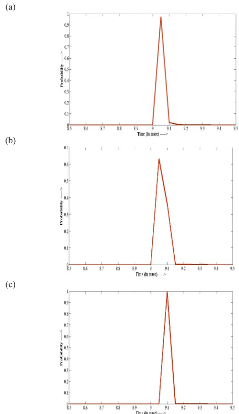
in our investigation. Fig. 1 illustrates the ISI distribution for the MHSN model with delay parameter

η = −

0.1

. Here, subfigure (a) depicts the ISI distribution for constant input stimulus of intensity 0.1. Subfigures (b) and (c) are the ISI distribution obtained for standard Gaussian distributed input stimulus and uniformly

distributed input stimulus in range [0,1], respectively. Qualitative behavior of these three ISI distributions is identical. As shown in Fig. 1, they are triangular distributed.

(a)

(b)

(c)

Fig. 1. ISI Distribution for the MHSN Model with (a) Constant Input. (b) Gaussian Distributed Input (c) Uniformly Distributed Input

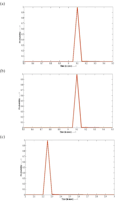
The ISI distribution for the considered model with stochastic input stimulus having mean

µ

and noise intensity

σ

is shown in Fig. 2. It has three subfigures corresponding to three different combination of parameter values

η

,

µ

and

σ

. Subfigure (a) depicts the ISI distribution for (

η

,

µ

,

σ

) = (−0.1,1,0.1). It has the qualitatively

behavior similar to the Fig. 1. In subfigure (b) and (c), we use (

η

,

µ

,

σ

) = (−1,1,0.1) and (

η

,

µ

,

σ

) = (−1,0.5,0.5) parameter

(a)

(b)

(c)

Fig. 2. ISI Distribution for the MHSN Model with stochastic input and (a)

η = −

0.1

(b)

η = −

1

(c)

η = −

1

In order to perform stability in next section, we compute the eigenvalues and steady state solution of the three dimensional MHSN model. Here, we also complete the phase plane analysis of the MHSN model.

III. s

TAbIlITy

A

nAlysIs

Investigation for the evolution of the behavior of state variables is studied under sensitivity analysis [13, 19, 24]. The MHSN model in extended space is a system of three coupled differential equations. It includes two important tasks. In first task, we compute the nullclines and steady state solution for the dynamical system where as second task deals with the phase plane analysis [13, 24]. In phase plane analysis, one analyzes the evolution of temporal behavior of state variables in phase space. In our study, we compute the nullclines, steady state solution, eigenvalues for the dynamical system and perform the phase plane analysis.

The MHSN model given as in Eqns. (11), (12) and (13), is a system of three coupled linear differential equations. Their matrix representation become [13]

.

Y AY B

=

+

₍₁₅₎

where

Y

=

( , ,

V U X

₀

)

T,

0

1 1

1 0

0

A

ab

η

η

−









=

_

−

_



₋







and

( ,0,0)

T

B

=

I

.

Nullclines and Steady State Solution:

Nullclines are the trajectories in phase space along which the behavior of the state variable changes [13, 24]. Intersection point of these trajectories yields the steady state solution [13]. Nullclines for the dynamical system can be computed by substituting the first derivative term equal to 0 [24]. Substitution of

Y

.

=

0

in the dynamical system defined in Eq. (15) results the required nullclines as

X U I

₀

− + =

0

,

bV U

− =

0

and

X V

₀

− =

0

. Nullclines for the investigated dynamical model result a system of three linear simultaneous equations. On solving these simultaneous equations, we get steady state solution

0

( ,_{V U X}S S, S) I , bI , I

b I b I b I

 

=  _{− − −} 

 , provided

b I

≠

. Here, we obtain a single steady state which can be a state or an unstable state which is investigated in next subsection phase plane analysis. Here, we further notice that the model parameter

a

and delay parameter

η

don’t affect the steady state solution of the model.

Computation for the Eigenvalues:

Let

λ

be an eigenvalue of the dynamical model (15), and then it can be computed by solving the equation

|

A

−

λ

I

| 0

=

[9, 22]. Its simplification results a cubic polynomial

3

₍₁

₎

2

_ab

₍

_ab

₁₎

₀

λ

+ +

η λ

+

λ

+

+

η

=

₍₁₆₎

Following the Cardano’s method for solving a cubic polynomial,

substitution of

1

3

Z

η

λ

= + −



_

+



_





into Eq. (16) and after some

simplification results [29]

3

1 2

0

Z

+

K Z K

+

=

₍₁₇₎

where 1 2

(1 ) 3

K =ab− +η and ₂ 2(1 ) 3(13 ) 9( 1)

9

ab ab

K = +η − +η + + .

Following Lal [29], here two cases exist.

Case 1: If

K

₁

=

0

i.e.

η = − ±

1

3

ab

Then eigenvalues for the investigated dynamical system become

α

,

αω

and

αω

2, where 13 2

( )

K

Case 2: Otherwise,

(

K

1

≠

0)

Then eigenvalues takes the form as

(

P P

₁

+

₂

)

,

(

P

₁

ω

+

P

₂

ω

2

)

and

(

P

₁

ω

2

+

P

₂

ω

)

, where 2 13 22 1

4

27

2

108

K

K

K

P

= −

+

−

−

and

3 2

2 1 2

2

K

₂

4

K

₁₀₈

27

K

P

= −

−

−

−

.

Phase Plane Analysis:

Phase space is a multidimensional space whose coordinates are the system variables [2, 13, 24]. It clearly depicts the dynamical behavior of the state variables [2, 13]. Dynamical system given in Eq. (15) has three state variables

V

,

U

and

X

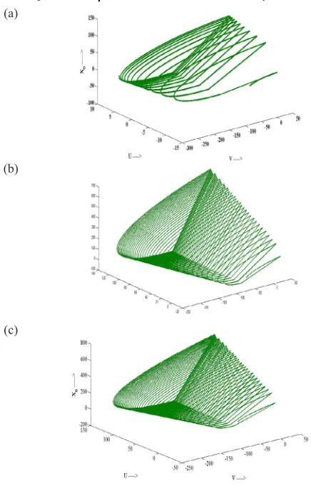
₀, thus we obtain a three dimensional phase space. We simulate this dynamical system same parameter values and simulation strategy as given in Section III.

In Fig. (3), subfigure (a), (b) and (c) show the temporal evolution of state variable with constant input, Gaussian distributed input and uniformly distributed input stimuli, respectively. Here, we observe the limit cycle oscillations generating a spiral structure due to the threshold constraint. This limit cycle oscillation is an important aspect in many biological processes [2].

(a)

(b)

(c)

Fig. 3. Phase Plane Analysis for the MHSN Model with (a) Constant Input (b) Gaussian Distributed Input (c) Uniformly Distributed Input

Fig. 4 shows the mutual behavior of state variables in the MHSN model with stochastic input stimulus. Here subfigure (a) reflects the evolution of state variables with small magnitude of delay parameter

0.1

η = −

and it qualitatively similar with the trajectories obtained in Fig. 3. We increase the magnitude of

η

to -1 and maintain the rest parameter values same as taken for Fig. (2). Here, once again, we obtain limit cycle oscillation but time duration of the cycle reduces. This finding suggests that the development of values in state variables occur in quicker time so that the spiking activity of the neuron increases. From Figs. 3 and 4, it is evident that the phase plane dynamics of the model does not alter due to the different kinds of input stimulus; however parameter

η

reduces the time duration of cycle.

(a)

(b)

(c)

Fig. 4. Phase Plane Analysis for the MHSN Model with stochastic input. (a) η= −0.1 (b) η = −1 (c) η = −1

IV. c

onclusIonAnd

f

uTuRe

w

oRk

The detailed investigation of the MHSN model in term of information processing capability reveals that the spiking activity of the considered neuron model is invariant under the influence of a large fluctuation of applied input stimulus. The state variable

X

₀of the model in extended space along with the delay parameter

η

curtails the variation in spiking activity. However, increase in the negative value of

which is independent of delay parameter. Choudhary et. al. [30] has shown that “the distributed delay has no effect on stationary state membrane potential distribution of a LIF neuron”. In addition, we say that the distributed delay has no effect on steady state solution of the threshold based linear neuron models.

Being the extension of Izhikevich neuron model [3], the MHSN model has the inherited property related to the implementation of after spiking reset condition at hardware level. Invariant spiking activity of the MHSN model reveals that the model is capable to handle the threshold variability and other noisy parameters like temperature increment in the chip. Lim et. al. [9] has implemented the neuristor-based leaky integrate-and-fire neuron model with aforementioned two critical issues to form an artificial neural network at hardware level. As the MHSN model is free from above stated prime issues, we recommend that the MHSN model should be a better choice for chip level implementation.

A

cknowledgMenT

The authors are extremely grateful to the reviewers whose comments have led to significant improvement in the quality of the paper.

R

efeRences

[1] A. Borst and F. E. Teunissen, “Information Theory and Neural Coding,” Nature Neuroscience, Vol. 2, No. 11, pp. 947-957, 1999.

[2] E. M. Izhikevich, “Neural Excitability, Spiking and Bursting,” International Journal of Bifurcation and Chaos, Vol. 10, No. 6, pp. 1171-1266, 2000. [3] E. M. Izhikevich, “Hybrid Spiking Models,” Philosophical Transactions of

The Royal Society A, Vol. 368, pp. 5061-5070, 2010.

[4] H. E. Plesser, “Aspects of Signal Processing in Noisy Neuron,” Dissertation submitted to Max-Planck-Institute, Gottigen, 1999.

[5] Joubert, Belhadj, O. Temam and R. Heliot, “Hardware Spiking Neurons Design: Analog or Digital?” IEEE World Congress on Computational Intelligence, 2012.

[6] D. J. Mar, C. C. Chow, W. Gerstner, R. W. Adams and J. J. Collins, “Noise Shaping in Populations of Coupled Model Neurons”, Proceedings of the National Academy of Sciences, USA, Vol. 96(18), pp. 10450-10455, 1999. [7] E. M. Izhikevich, “Simple Model of Spiking Neurons,” IEEE Transactions

on Neural Networks, Vol. 14, No. 6, pp. 1569-1572, 2003.

[8] E. M. Izhikevich, “Which Model to Use for Cortical Spiking Neurons?” IEEE Transactions on Neural Networks, Vol. 15, No. 5, pp. 1063-1070, 2004.

[9] H. Lim, V. Kornijuck et. al., “Reliability of Neuronal Information Conveyed by Unreliable Neuristor Based Leaky Integrate-and-Fire Neurons: A Model Study,” Nature: Scientific Reports, 5:09776 , DOI: 10.1038/srep09776, pp. 1-15, 2015.

[10] L. S. Liao and G. Chen, “Bifurcation Analysis on a Two Neuron System with Distributed Delay in the Frequency Domain”, Neural Network, Vol. 17, Issue 4, pp. 1654-1664, 2004.

[11] W. Gerstner and W. M. Kistler, “Spiking Neuron Models: Single Neurons, Populations, Plasticity,” Cambridge University Press, 2002.

[12] V. B. Semwal, M. Raj and G. C. Nandi, “Biometirc gait identification based on a multilayer perceptron”, Robotics and Autonomous Systems, Vol. 65, pp. 65-75, 2015.

[13] E. M. Izhikevich, “Dynamical Systems in Neuroscience: The Geometry of Excitability and Bursting,” The MIT Press, 2007.

[14] A. Fairhall, E. S. Brown and A. Barreiro, “Information Theoretic Approaches to Understanding Circuit Function,” Neurobiology, Vol. 22, pp. 653-659, 2012.

[15] E. M. Izhikevich and G. M. Edelman, “Large-Scale Model of Mammalian Thalamocortical Systems,” PNAS, Vol. 105, No. 9, pp. 3593-3598, 2008. [16] M. I. Rabinovich, P. Varona, A. I. Selverston and H. D. I. Abarbanel,

“Dynamical Principles in Neuroscience,” Reviews of Modern Physics, Vol. 78, No. 4, pp. 1213-1265, 2006.

[17] S. Millner, A. Grubl, K. Meier, J. Schemmel and M. Schwartz, “A VLSI Implementation of the Adaptive Exponential Integrate-and-Fire Neuron

Model,” Advances in Neural Information Processing Systems, Vol. 23, pp. 1642-1650, 2010.

[18] A. V. Holden, “Models of the Stochastic Activity of Neurons”, Lecture Notes in Biomathematics, Springer, 1976.

[19] N. MacDonald, “Time Lags in Biological Models”, Lecture Notes in Biomathematics, Springer, 1978.

[20] Karmeshu, V. Gupta and K. V. Kadambari, “Neuronal model with distributed delay: analysis and simulation study for gamma distribution memory kernel,” Biological Cybernatics, Vol. 104, pp. 369-383, 2011. [21] S. K. Sharma and Karmeshu, “Neuronal Model With Distributed

Delay: Emergence of Unimodal and Bimodal ISI Distributions”, IEEE Transactions on Nanobioscience, Vol. 12, No. 1 pp. 1-12, 2013.

[22] S. K. Bharti, S. K. Choudhary and J. Singh, “Analytical Solution for Izhikevich Hybrid Spiking Neuron Model with Distributed Delay,” Utthan: The Journal of Applied Sciences & Humanities, Vol. 1, No. 2, pp. 19-24, 2014.

[23] S. K. Choudhary, K. Singh and H.O.S. Sinha, “Spiking Activity of Hybrid Spiking Neuron Model in DDF”, in International Conference on Research in Intelligent Computing in Engineering (RICE 2016), 08-09 April 2016, Nagpur, India , pp. 261-264.

[24] H. Smith, “An Introduction to Delay Differential Equations With Applications to the Life Sciences,” Texts in Applied Mathematics, Vol 57, Springer, Berlin, 2011.

[25] H. R. Wilson, “Spikes, Decision and Actions,” Oxford University Press, 2005.

[26] L. F. Abbott and P. Dayan, “Theoretical Neuroscience: Computational and mathematical modeling of neural systems”, The MIT press, 2001. [27] P. E. Kloeden and E.Platen, “Numerical Solution of Stochastic Differential

Equations,” Springer, Berlin, 1992.

[28] P. Glasserman, “Monte Carlo Methods in Financial Engineering”, Springer, 2004.

[29] R. J. Lal, “Algebra,” Volume II, Shail Publication, Allahabad, 2002. [30] S. K. Choudhary, K. Singh and V. K. Solanki, “Spiking Activity of a LIF

Neuron in Distributed Delay Framework”, in International Journal of Artificial Intelligence and Interactive Multimedia (In Press).

Saket Kumar Choudhary obtained his master degrees in Mathematics from the University of Allahabad, Allahabad, India in 2005, Master of Computer Application (MCA) from UPTU, Lucknow, India in 2010, Master of Technology (M.Tech) from Jawaharlal Nehru University, New Delhi, India in 2014. He is finishing his doctorate in School of Computer and Systems Sciences, Jawaharlal Nehru University, New Delhi, India. His research interest includes mathematical modeling and simulation, dynamical systems, computational neuroscience: modeling of single and coupled neurons, computer vision and digital image processing.