Maximum Likelihood for Gaussian Process Classification and
Generalized Linear Mixed Models under Case-Control
Sampling
Omer Weissbrod [email protected]
Epidemiology Department
Harvard T.H. Chan School of Public Health Boston, MA 02115, USA
Shachar Kaufman [email protected]
Department of Statistics and Operations Research School of Mathematical Sciences
Tel-Aviv University Tel-Aviv 6139101, Israel
David Golan [email protected]
Viz.ai
Tel-Aviv 6121001, Israel
Saharon Rosset [email protected]
Department of Statistics and Operations Research School of Mathematical Sciences
Tel-Aviv University Tel-Aviv 6139101, Israel
Editor:Ryan Adams
Abstract
Modern data sets in various domains often include units that were sampled non-randomly from the population and have a latent correlation structure. Here we investigate a com-mon form of this setting, where every unit is associated with a latent variable, all latent variables are correlated, and the probability of sampling a unit depends on its response. Such settings often arise in case-control studies, where the sampled units are correlated due to spatial proximity, family relations, or other sources of relatedness. Maximum likeli-hood estimation in such settings is challenging from both a computational and statistical perspective, necessitating approximations that take the sampling scheme into account. We propose a family of approximate likelihood approaches which combine composite likelihood and expectation propagation. We demonstrate the efficacy of our solutions via extensive simulations. We utilize them to investigate the genetic architecture of several complex disorders collected in case-control genetic association studies, where hundreds of thousands of genetic variants are measured for every individual, and the underlying disease liabilities of individuals are correlated due to genetic similarity. Our work is the first to provide a tractable likelihood-based solution for case-control data with complex dependency struc-tures.
Keywords: Gaussian Processes, Expectation Propagation, Composite Likelihood, Selec-tion Bias, Linear Mixed Models
c
1. Introduction
In the analysis of scientific data, a common phenomenon is the existence of complex depen-dencies between analyzed units. This is encountered in diverse fields such as epidemiology, econometrics, ecology, geostatistics, psychometrics and genetics, and can arise due to spatial correlations, temporal correlations, family relations, or other sources of heterogeneity (Pfeif-fer, 2008; Rabe-Hesketh et al., 2005; Bolker et al., 2009; Rabe-Hesketh et al., 2004; Yang et al., 2014; Burton et al., 1999; Diggle et al., 1998). This idea is often captured through the use of Gaussian processes (GPs; Rasmussen and Williams 2006) or equivalently, through generalized linear mixed models (GLMMs; McCulloch et al. 2008) or latent Gaussian mod-els (Fahrmeir and Tutz, 2001). Such modmod-els associate sampled units with latent variables, and express the dependencies through covariance matrices of latent variables.
A second important concept is that of ascertainment, where the probability of sampling a unit depends on its response. Ascertainment is especially common in case-control studies where a binary response variable has a rare outcome, such as a rare disease, leading to oversampling of disease cases relative to their population prevalence (Breslow, 1996).
In this paper we consider situations that contain both elements—a complex covariance structure and case-control sampling—and the statistical modeling solutions available for these situations. Our interest lies in an extreme form of this combination, involving:
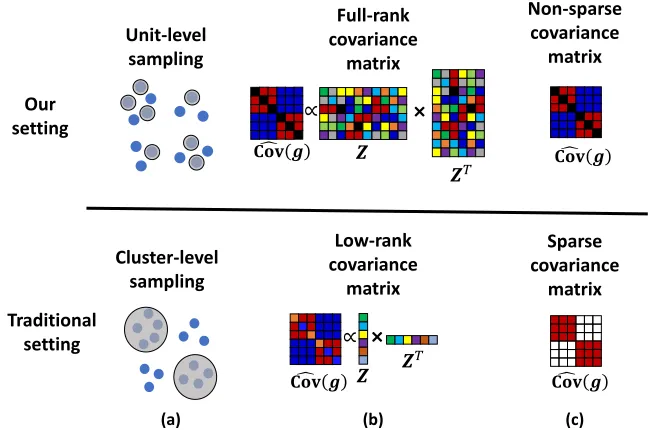
(a) Unit-level ascertainment, where the sampling probability of a unit depends only on its response (Figure 1a). This stands in contrast to common study designs such as family studies (Neuhaus et al., 2002), ascertained longitudinal studies (Liang and Zeger, 1986) or clustered case-control studies (Neuhaus and Jewell, 1990). In such studies each cluster is either entirely selected or entirely omitted from the study, such that the dependency structure in the sample and in the population are the same.
(b) A full-rank covariance matrix, indicating that dependencies cannot be captured by a small number of variables (Figure 1b). Such settings are common in modern data sets due to either high-dimensional settings or to the use of kernels or basis expansions, which implicitly project a small number of features into a large (possibly infinite-dimensional) space (Diggle et al., 1998; Rasmussen and Williams, 2006).
(c) A non-sparse covariance matrix, indicating that all units are correlated (Figure 1c). Such settings exacerbate both the computational challenge, because the density does not factorize into multiplicative terms, and the statistical challenge, because classic statistical theory requires a large number of independent units.
Special cases of this combination have been addressed in the literature (Glidden and Liang, 2002; Epstein et al., 2002; Neuhaus et al., 2006, 2014), but to our knowledge, there is a limited set of available solutions for the general setting, which is indeed very challenging.
Traditional setting
Cluster-level sampling Unit-level sampling
Our setting
Low-rank covariance
matrix
∝
×
Full-rank covariance
matrix
𝒁
𝒁𝑇
𝒁𝑇
𝒁
×
∝ 𝐂𝐨𝐯 𝒈
𝐂𝐨𝐯 𝒈
Sparse covariance
matrix Non-sparse
covariance matrix
𝐂𝐨𝐯 𝒈
𝐂𝐨𝐯 𝒈
(a) (b) (c)
Figure 1: The properties that are unique to our setting of interest (top row) compared to more traditional settings (bottom row). (a) Unit-level sampling, where the decision whether to sample a unit depends only on their response, in contrast to studies that either sample or omit an entire cluster of units. (b) A full-rank covariance matrix of latent variables, indicating a complex dependency structure. (c) A non-sparse covariance matrix, indicating that the latent variables of every pair of units are correlated.
et al., 2014; Weissbrod et al., 2015), estimating disease heritability (Yang et al., 2010; Golan et al., 2014; Weissbrod et al., 2018), risk prediction (Zhou et al., 2013; Golan and Rosset, 2014; Weissbrod et al., 2016), and more.
(Lee et al., 2011; Hayeck et al., 2015; Weissbrod et al., 2015; Chen et al., 2016; Jiang et al., 2016a).
Similar settings arise in other scientific domains, where case-control sampling and a full-rank, non-sparse covariance structure are observed. Prominent examples include disease mapping studies with a smoothing kernel (Diggle et al., 1998; Kelsall and Diggle, 1998; Held et al., 2005) and GP-based classification of data collected in case-control studies (Chu et al., 2010; Ziegler et al., 2014; Young et al., 2013). The analyses employed in these examples often ignore the effects of case-control sampling, a practice we would like to avoid and whose fundamental flaws we discuss and illustrate below.
The problem we consider poses substantial statistical and computational challenges. The main statistical framework for inference with binary responses and latent variables are GP classifiers, which are mathematically equivalent to latent Gaussian models, and recover GLMMs as a special case when using a linear kernel. Such models provide a likelihood-based solution but can pose significant computational difficulties. Modern approach to alleviate computational difficulties include (1) Pairwise likelihood (PL; Renard et al. 2004), which approximates the joint distribution of all variables as a product of marginal distributions of pairs of variables; (2) Expectation propagation (EP) (Minka, 2001; Seeger, 2005), which replaces multiplicative terms in the distribution with simpler terms from an exponential family distribution; (3) Variational approximation (Opper and Archambeau, 2009; Hens-man et al., 2015), which approximates the distribution with the closest distribution from a more tractable class; (4) Markov chain Monte Carlo (MCMC) sampling combined with thermodynamic integration (Kuss and Rasmussen, 2005; Nickisch and Rasmussen, 2008; Gelman and Meng, 1998), and (5) Laplace approximation (Tierney and Kadane, 1986; Raudenbush et al., 2000) and its close variant, penalized quasi likelihood approximation (Breslow and Clayton, 1993; Wolfinger and O’connell, 1993), which approximate the distri-bution as a Gaussian distridistri-bution via a second-order Taylor expansion. Of these, PL and EP have proved to often outperform the alternatives (Kuss and Rasmussen, 2005; Nickisch and Rasmussen, 2008; Varin et al., 2011) and thus form the basis of our proposed approach.
The main approach for statistical inference in the presence of ascertainment is called
ascertained maximum likelihood (AML). AML consists of defining a binary variable indi-cating inclusion in the study for every unit, and conditioning the analysis on these variables (Scott and Wild, 2001). However, none of the above GP approximation methods is suit-able for AML inference. The only existing method that is both scalsuit-able and statistically sound is a method-of-moments approach called phenotype-correlation-genotype-correlation (PCGC; Golan et al. 2014). However, this approach is not likelihood-based and thus cannot naturally be used for model comparison, inference, prediction, and hypothesis testing.
2. Formal Problem Description
Here we provide a formal description of our problem and the statistical and computational challenges.
2.1. Gaussian Processes / Generalized Linear Mixed Models
We are presented withn units, with each unitihaving cfeatures Xi ∈Rc associated with
fixed (non-random) effects β∈Rc,m additional features Zi ∈Rm that are not associated
with fixed effects, and an outcome variable yi (here we consider binary outcomes, but the
framework can also be applied to other types). We associate every unit i with a latent variablegi(Zi) that depends on Zi such thatP(yi = 1 |Xi, gi,β) =h XiTβ+gi
,where
h(·) is a likelihood function (which is closely related to an inverse link function in GLMM terminology), such as probit or logit.
GPs impose a Gaussian process prior over the the functional form of the latent vari-ables, g∼ GP(0, k(·,·;θ)),wherek(·,·;θ) is a kernel function parameterized by θ. This indicates that for every finite set of unitsi= 1. . . n, the vector g= [g1(Z1), . . . , gn(Zn),]T
follows a multivariate normal distribution:
g ∼ N(0,K(Z;θ)),
whereK, which is non-sparse and full-rank in our setting, has entries Kij =k(Zi,Zj;θ).
GLMMs are a class of models that are mathematically equivalent to GPs with linear kernels, i.e.,Kij =θZiTZj, whereθis a scalar hyperparameter called avariance component.
GLMM literature typically uses the alternative notationgi =ZiTb, whereb∼ N
0,√θI
is a vector ofrandom effects. The equivalence can be extended to non-linear kernels by making use of Mercer’s theorem (K¨onig, 2013), which allows expressing every kernel function as a (possibly infinite) linear combination of basis functions, k(Zi,Zj;θ) = P∞r=1φr(Zi;θ)·
φr(Zj;θ). Hence, every GP can be written as a GLMM over the feature space {φr(Z)}
with iid random effectsbr∼ N(0,1). GLMMs can also be defined with non-normal random
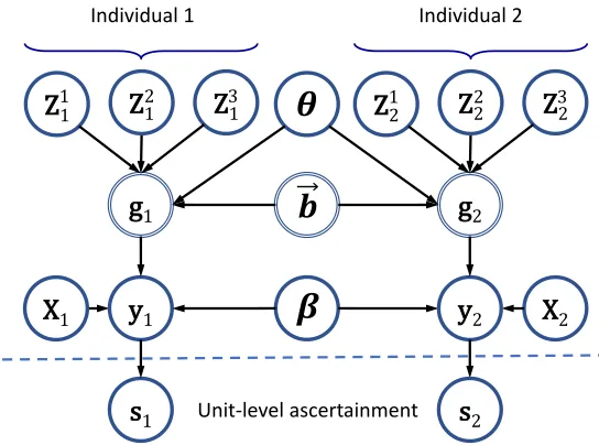
effects, in which case the equivalence with GPs breaks down, but we do not consider such models here. We focus on linear kernels because we are interested in extremely high-dimensional settings, where non-linear kernels often overfit (Weissbrod et al., 2016). A graphical model of GPs and GLMMs is shown in Figure 2.
Our main aim in this work is estimating the kernel hyperparameters θ (i.e., training the model). Given a vector of observed outcomes y= [y1, . . . , yn]T and the matricesX =
[X1, . . . ,Xn]T,Z= [Z1, . . . ,Zn]T, the GP likelihood is given by:
L(β,θ) =P(y |X,Z,θ,β) = Z
P(g|Z,θ)Y
i
P(yi|Xi, gi,β)dg. (1)
X
2g
2Z
21Z
22Z
32g
1Z
1Z
1Z
1X
11 2 3
y
2y
1s
1 Unit-level ascertainments
2Individual 1 Individual 2
𝜽
𝜷
𝒃
Figure 2: A directed graphical model for a GP with one featureX associated with a fixed effectβ, three features Z1, Z2,Z3 associated with an implicit vector of random effects ~b and with a hyperparameter θ, and two sampled units (indicated by subscript indices) with latent variablesg1,g2and observed responsesy1,y2. Also shown is the extension to unit-level ascertainment, which consists of adding a sampling indicatorsi that depends onyi and is equal to 1 for every sampled unit.
Latent (non-observed) random variables are marked with a double-lined border.
2.2. The Implications of Ignoring Ascertainment in GPs
Up until now we implicitly assumed thatnunits were sampled completely at random from an underlying population. We now assume that the sample is ascertained, i.e., that the probability of sampling cases (units withyi = 1) and controls (yi= 0) is different.
We first demonstrate that using GPs while ignoring ascertainment leads to nonsensical conclusions which stand in contrast to fundamental motivations for GP use, like the central limit theorem. We focus on binary GPs, which can be formulated according to the liability threshold model (Dempster and Lerner, 1950). Under this model, every unit ihas a latent liabilityli =gi+i, wherei is an iid latent residual variable whose distribution depends on
the likelihood function (e.g. normally distributed for probit, or logit distributed for logit), and unitiis a case (having yi= 1) if and only ifli > tfor some cutofft. Theprevalence K
is the proportion of units in the population having li > t. We emphasize that a normally
distributed i is completely equivalent to a standard GP with a probit likelihoodh(·).
It is common to use likelihood functions associated with a smooth and symmetrically distributed i, such as logit or probit, which leads to a smooth and symmetric distribution
of liabilities in the population. However, due to the ascertainment mechanism, the liabili-ties and latent variables gi in an ascertained sample follow a non-symmetric and possibly
2
1
0
1
2
3
4
Liability
0.0
0.5
1.0
1.5
Sample density
0.1% Prev.
1% Prev.
10% Prev.
50% Prev.
2
1
0
1
2
3
4
Liability
0.0
0.2
0.4
0.6
0.8
Population density
2
1
0
1
2
3
Latent variable
Assume normality in population
(a)
0.0
0.2
0.4
Sample density
2
1
0
1
2
3
Latent variable
Assume normality in sample
(b)
0.00
0.25
0.50
0.75
1.00
Population density
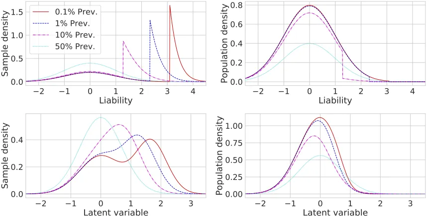
Figure 3: The implications of assuming normality of latent variables in the population from which units are sampled (panel a) or in a case-control study (panel b), for a GP with a probit likelihood and a sample consisting of 50% cases. The liability is given by li = gi +i, gi, i ∼ N(0,
√
0.5). Units with liabilities greater than their (1-prevalence) population quantile are cases. (a) When assuming normality in the population, latent variables and liabilities in a case-control study are not normally distributed (unless the cases prevalence is 50%, in which case there is no ascertainment). (b) When naively assuming normality of latent variables in a case-control study, the latent variables and the liabilities arenot normally dis-tributed in the population from which the data was sampled, in contradiction to the liability threshold model. Specifically, the liabilities distribution is discontin-uous, and the latent variables distribution has a heavy left tail. All distributions were computed analytically by conditioning on the sampling indicators defined in Section 2.3.
studies. Many studies in practice ignore the complexities above, and instead use common likelihood functions such as a logit or a probit in case-control studies (e.g. Chen et al. 2016; Jiang et al. 2015; Kramer et al. 2017; Qi et al. 2017). However, this solution implies a non-symmetric and discontinuous distribution of latent variables in the population from which units are sampled, in stark contrast to the central limit theorem assumptions (Figure 3b). Thus, ignoring the ascertainment scheme in GPs may lead to nonsensical probabilistic settings under common assumptions.
2018), inaccurate risk prediction (Golan and Rosset, 2014) and loss of power in hypothesis testing (Weissbrod et al., 2015; Hayeck et al., 2015; Yang et al., 2014).
2.3. Modeling Ascertainment in GPs
Analysis of ascertained data is typically performed by (1) defining a binary sampling in-dicator si for every uniti such that si depends only onyi (Figure 2); and (2) performing
all statistical inference tasks conditional on s1 = 1, . . . , sn = 1. This requires
specify-ing two numbers: the samplspecify-ing probabilities of cases P(si = 1|yi = 1) and of controls
P(si = 1|yi = 0). There are two main approaches for estimating the hyperparameters
θy|X,Z of the distribution P(y|X,Z) with such indicators, differing with respect to how the sampling probabilities are determined.
Maximum profile likelihood estimatesθy|X,Z by jointly maximizing the so-called profile likelihood P(y|X,Z, s1 = 1, . . . , sn= 1) over bothθy|X,Z and the nuisance hyperparame-ters θs|y of the distributions P(si= 1|yi) of every possible value of yi, i.e., ˆθy|X,Z, ˆθs|y=
argmaxθ
y|X,Z,θs|yP y |X,Z, s1 = 1, . . . , sn= 1,θy|X,Z,θs|y
(Scott and Wild, 2001). The resulting estimator is maximally efficient as it attains the Cram´er-Rao lower bound.
Ascertained Maximum Likelihood (AML) estimatesθy|X,Z using a pre-specified assign-mentθs|y =θ0s|y, i.e., ˆθy|X,Z = argmaxθy|X,Z P
y |X,Z, s1= 1, . . . , sn= 1,θy|X,Z,θs|y0
(Scott and Wild, 1997). For a binary outcome with a population prevalence K and an in-sample prevalence P, any assignment θ0s|y obeying the constraint P(si=1|yi=0)
P(si=1|yi=1) =
K(1−P) (1−K)P
guarantees consistent estimates (i.e., estimators converge to the true parameter values as sample size tends to infinity if the model is true), because it yields the observed case-control ratio in expectation. This approach is often termed pseudo likelihood or conditional like-lihood (Manski, 1981; Hsieh et al., 1985), but as both terms have alternative meanings in GLMM literature, we use the term ascertained likelihood instead. AML is less statistically efficient than maximum profile likelihood, in the sense that the estimator has a larger vari-ance. However, the loss of efficiency has been shown to be negligible in practice (Wild, 1991; Scott and Wild, 1997). AML has previously been used for family-based studies (Glidden and Liang, 2002; Epstein et al., 2002), but to our knowledge it has not been used under the combination of a dependency structure and unit-level sampling.
To combine GPs with the AML framework, we define the ascertained GP likelihood and apply Bayes’ law as follows:
L∗(β,θ) =P(y |X,Z,s= 1,θ,β) = P(y |X,Z,θ,β)
P(s= 1|X,Z,θ,β) Y
i
P(si = 1|yi), (2)
where s = 1 is a shorthand notation for s1 = 1, . . . , sn = 1 and θy|X,Z = {θ,β}. The last term in the rhs of Equation 2 is considered known under AML and requires no special treatment. The numerator is the likelihood of a standard GP under no ascertainment, and the denominator is the likelihood of a GP in which the outcome issi instead of yi. A naive
3. Approximate Inference in GPs under Ascertainment
We now propose two methods for approximate inference in GPs under ascertainment.
3.1. Ascertained Pairwise Likelihood
PL is a composite likelihood approximation, which approximates multivariate joint densities via products of marginal bivariate densities: (Varin et al., 2011; Renard et al., 2004):
P(y |X,Z,θ,β)∝∼Y
i6=j
P(yi, yj |Xi,Xj,Zi,Zj,θ,β), (3)
where i,j iterate over all pairs of units, and ∝∼ indicates approximate proportionality with respect to the hyperparameters θ, β. The maximum pairwise likelihood estimate is ap-proximately the maximum likelihood estimate. PL is computationally efficient owing to its quadratic dependency on the sample size, and is statistically consistent under suitable regularity conditions (Varin et al., 2011).
Ascertained PL (APL) is an extension of PL that approximates the ascertained likeli-hood in Equation 2 by modifying Equation 3 to condition on s= 1 :
P(y |X,Z, s= 1)∝∼Y
i6=j
P(yi, yj |Xi,Xj,Zi,Zj, si= 1, sj = 1)
= Y
i6=j
P(yi, yj |Xi,Xj,Zi,Zj)
P(si=sj = 1 |Xi,Xj,Zi,Zj)
P(si =sj = 1|yi, yj),
where P(si =sj = 1|yi, yj) = P(si= 1|yi)P(sj = 1|yj) are known constants which can
be ignored, and we omitted the hyperparametersβ,θ for brevity. The terms in the numer-ator and the denominnumer-ator can be separately evaluated as in standard PL, where we treat the denominator as a GP with a suitable likelihood function. Unlike Equation 2, the evalu-ation of the ratio is accurate since both the numerator and denominator can be computed exactly. In certain settings, PL evaluation can be substantially accelerated via a Taylor approximation around ZiTZj = 0, which enables factoring each bivariate distribution into
a product of marginal distributions (Appendix A).
3.2. Ascertained Expectation Propagation
EP is a popular approach for approximating complex distributions by iteratively replac-ing every multiplicative term in the joint distribution of the observed and latent vari-ables with a simpler term from an exponential family distribution (Minka, 2001; Ras-mussen and Williams, 2006; Seeger, 2005). This joint distribution in GPs is given by
P(g|Z,θ)Q
iP(yi|Xi, gi,β). EP replaces every term in this product by an unnormalized
Gaussian, P(yi|Xi, gi) ≈ ti(gi) ,riN (gi;αei,eγi), where we omitted the hyperparameters β, θ for brevity, and the site parameters ri,αei, eγi implicitly depend on Xi, yi and β. EP iteratively updates the termsti(gi), such that each term minimizes the generalized Kullback
Leibler divergence (GKL) between the functions q−i(gi)ti(gi) and q−i(gi)P(yi|Xi, gi) (i.e.,
the KL divergence between these functions after standardizing them to integrate to unity), where the cavity distribution q−i(gi) ∝
R
P(g|Z)Q
j6=itj(gj)dgj6=i represents the current
Given an EP approximation, the GP likelihood can be approximated as:
P(y |X,Z)≈
Z
P(g|Z)Y
i
ti(gi)dg.
This expression can be evaluated analytically because it is an integral of a product of (unnormalized) Gaussian densities. EP has proven to consistently outperform alternative approximation methods for binary data (Nickisch and Rasmussen, 2008), and recent theo-retical analysis has demonstrated that is is statistically consistent under certain modeling assumptions (Dehaene and Barthelm´e, 2016, 2018).
Ascertained EP (AEP) is our proposed method to generalize standard EP to handle ascertainment. AEP approximates the ascertained likelihood in Equation 2 by replacing the standard EP step with a modified step that equates the functions R
q−i(gi)ti(gi)dgi
and
R
q−i(gi)P(yi,si|gi,Xi)dgi
R
q−i(gi)P(si|gi,Xi)dgi . Unlike standard EP, we cannot minimize the GKL divergence
beteween these functions, because this will lead to the same solution as standard EP, up to a scaling constant. Instead, AEP finds the unnormalized Gaussian ti(gi) which makes
these functions and their first two partial derivatives with respect to µ−i (the mean of the
Gaussianq−i(gi)) have the same value when evaluated atµ−i (see Appendix B for details).
EP is a special case of AEP, because the proposed step objective coincides with the standard EP objective in the absence of ascertainment (i.e., when P(si|yi) is a constant
regardless of yi). To see this, observe that EP minimizes the GKL divergence between
ˆ
m(gi) , q−i(gi)P(yi|gi,Xi) and ˜m(gi) , q−i(gi)·ti(gi). Since ˜m(gi) is an unnormalized
Gaussian, EP minimizes the GKL divergence by equating its zeroth, first and second mo-ments with those of ˆm(gi) (Rasmussen and Williams, 2006). Hence, standard EP requires
computing the mean ˆµi and variance ˆσi2 of ˆm(gi). A straightforward but lengthy derivation
shows that we can compute these quantities as follows:
ˆ
µi =
∂ ∂µ−i
log
Z ˆ
m(gi)dgi
σ−i2 +µ−i
ˆ
σ2i = ∂ 2
∂(µ−i)2
log
Z ˆ
m(gi)dgi
σ−i2 2 +σ−i2 ,
whereµ−i, σ2−i are the mean and variance of the Gaussian q−i(gi), and the derivatives are
evaluated at the actual value ofµ−i. Hence, there is a one-to-one correspondence between
the first two moments of ˆm(gi) and its first two partial derivatives with respect toµ−i(when
evaluated at µ−i). Consequently, each step of standard EP can alternatively be described
as imposing the constraint that the zeroth, first and second derivatives of the integrals of ˜
m(gi) and ˆm(gi) with respect to µ−i are the same. This is the same constraint used in
AEP. Hence, EP and AEP coincide in the absence of ascertainment, where P(si = 1|yi) is
constant regardless of the value ofyi.
The sampling variance of the AEP maximum likelihood estimator can be estimated effi-ciently via jackknife sampling, by reusing the functionsti(gi) (Opper and Winther, 2000; Qi
rotations (Seeger, 2004). A formal analysis of AEP is difficult because there are relatively few theoretical guarantees for standard EP, which is a special case of AEP, except under relatively strong assumptions (Dehaene and Barthelm´e, 2016, 2018). However, we sketch a heuristic argument supporting the objective function of AEP in Appendix B.
4. Results
We evaluated the performance of our methods using extensive simulations and real data analysis. We first describe our simulation studies, and then present the results obtained on real data.
4.1. Simulations Overview
We simulated data that closely mimics real GWAS-CC using the liability threshold model, where each individual has liability li = XiTβ+gi +i, gi is a GP latent variable, and
individuals withli greater than some cutoff are cases. In most simulations we used a linear
kernel with a single hyperparameter, θ = {σ2
g}, though we also investigate radial basis
function (RBF) kernels below. Our aim was estimating the hyperparameter σ2g, which we call a variance component. Importantly, σg2/var(li) is an estimator of genetic heritability,
defined as the proportion of var(li) explained by genetics.
We simulated genetic data based on single nucleotide polymorphisms (SNPs), which can be encoded as 0/1/2, according to the number of minor alleles carried by an individual at a specific position in the genome. We first generated a minor allele frequencyfj ∼ U(0.05,0.5) for every SNPj, and then sampled a matrixZ of SNP, such thatZij ∼Bin(2, fj). Finally,
we standardized each column in the matrixZ by subtracting the mean and dividing by the standard deviation corresponding to its allele frequency.
To simulate unit-level ascertainment, we (1) generated a population of 1,000,000 individ-uals, where for every individualiwe generated a vector of standardized genotypesZi ∈Rm
as described above, and a vector Xi∼ N(0,I) ∈ Rc representing additional standardized
risk factors such as sex or age; (2) generated vectorsb∼ N0,qσ2
g/mI
of random effects,
and β∼ N0,pσ2
c/cI
of fixed effects; (3) assigned a latent variable gi = ZiTb and a
liability li = gi+XiTβ+i to every individual i, where i∼ N
0,q1−σ2
c−σg2
iid; (4) defined all individuals with li greater than the 1−K quantile of the liability distribution
as cases (i.e., yi = 1), where K is the desired prevalence; and (5) selected a subset of n2
cases and n2 controls for the case-control study, where n is the desired study size. Unless stated otherwise, we usedm= 500, n= 500, K= 1%, σg2 = 0.25, σ2c = 0.25, andc= 1. We generated 100 datasets for each unique combination of evaluated settings.
We evaluated three likelihood-based methods: AEP, APL and plain EP, which does not account for ascertainment. We additionally evaluated the moment-based method PCGC, which is considered the state of the art approach for hyperparameter estimation in genetic case-control studies (Golan et al., 2014). We estimated hyperparameters in the likelihood-based methods via maximum likelihood, and in PCGC by finding the values that minimize the squared loss between the observed and expected values of cov(yi, yj) across all pairs of
ascertainment-0.05
0.25
0.45
True hyperparameter
(a)
0.0
0.2
0.4
0.6
0.8
1.0
Estimated hyperparameter
Method
AEP
APL
PCGC
Plain EP
0.1%
1%
5%
10%
50%
Trait prevalence
(b)
0.0
0.2
0.4
0.6
0.8
1.0
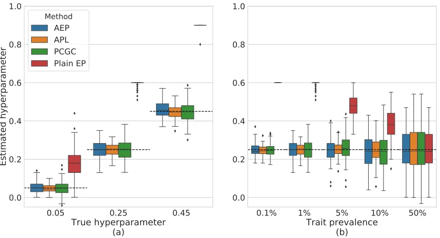
Figure 4: Evaluating hyperparameter estimation accuracy. Shown are box-plots depicting the estimates of each method across 100 different simulations, under data sets with an equal number of cases and controls, and a model with a single scale hyperparameter σg2. The dashed horizontal lines represent the true underlying values ofσg2used to generate the data. (a) AEP, APL and PCGC provide accurate estimates of σg2 when the true trait prevalence (the prevalence of cases in the population) is 1%, for various values of σ2
g, whereas plain EP is severely biased.
(b) All methods except for plain EP accurately estimate σg2 regardless of the underlying trait prevalence. Plain EP is accurate only when the prevalence is 50%, in which case there is no ascertainment.
aware generalized estimating equations (AGEE) approach that we developed, and then adjusted the affection cutoffs accordingly (Appendix C).
4.2. Simulation Studies: Estimating hyperparameters
Our first experiment evaluated variance component estimation accuracy. All methods ex-cept plain EP yielded empirically unbiased estimates, whereas plain EP was severely biased (Figure 4a). We also generated data under different prevalence values K and verified that all methods except plain EP remained accurate regardless ofK, whereas plain EP was only accurate whenK = 0.5, in which case there is no ascertainment (Figure 4b).
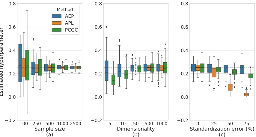
In the next experiment we examined sensitivity to sample size n and dimensionality
100 250 500 1000 2500
Sample size
(a)
0.2
0.0
0.2
0.4
0.6
0.8
Estimated hyperparameter
Method
AEP
APL
PCGC
5 10 50 500 1000
Dimensionality
(b)
0.2
0.0
0.2
0.4
0.6
0.8
0 25 50 75
Standardization error (%)
(c)
0.2
0.0
0.2
0.4
0.6
0.8
Figure 5: Investigating how hyperparameter estimation performance is affected by sample size, data dimensionality and modeling violations. (a) All the methods gain accu-racy as the sample size increases. The sampling variance of PCGC is consistently larger, because it uses a moment-based rather than a likelihood-based estimator. (b) All the methods gain accuracy as dimensionality increases. AEP is substan-tially more accurate than the other methods in the presence of a small number of features, because the other two methods use a first-order Taylor expansion around ZZT = I, which is less accurate in the presence of a small number of features. APL estimates for numbers <50 are equal to 1.0, and are omitted for clarity. (c) AEP is robust to feature standardization misspecification (see main text), whereas PCGC is moderately sensitive and APL is highly sensitive.
more accurate when m < 50 (Figure 5b). This is because the other two methods use a first-order Taylor expansion around ZZT =I, which is less accurate when m is small.
We also examined robustness to modeling violations by introducing noise into the feature standardization procedure. We multiplied the estimated frequency of every binary variable
j by rj ∼ U
1
1+e,1 +e
Next, we examined estimation accuracy under non-linear kernels. We generated data with a scaled RBF kernel, Kij =σg2exp
− kZi−Zjk2/ 2γ2
, and estimated the
hyper-parameters θ = σ2g, γ . Our generative model used σg2 = 0.25, γ = 0.5, and the same values as in the linear kernel simulations for all other parameters, except for restricting to
m=10 normally-distributed features. This is because RBF kernels tend to overfit under a largem, yielding Kij that is very close to either 0 orσ2g regardless ofZ.
A technical challenge of the RBF experiments is that our simulations first generate true latent variables gi for a population of 1M units. This requires computing a 1M ×
1M RBF covariance matrix K and sampling g = [g1, . . . , gn]T from N (0,K), which is
computationally intractable under a non-linear kernel. Instead we (1) generated a base population of 10K feature vectors Zi and a corresponding 10K×10K RBF kernel matrix
K10K; (2) sampled 10K gi values from N(0,K10K); and (3) created a population of 1M
units, such that each unit has a vector Zi and a correspondinggi value selected at random
from the base population, along with uniquely generated values ofXi andi. Afterwards we
followed the same procedure as in the linear kernel simulations of (1) generating a liability
li =XiTβ+gi+ifor each unit; (2) determining the liability cutoff according to the desired
prevalence; and (3) samplingn/2 cases andn/2 controls. We modified PCGC and APL to ignore pairs of units with identical features in these experiments.
AEP was empirically unbiased in the RBF experiments, having an average estimation bias of -0.016 (stdev 0.068) forσ2g and of 0.022 (stdev 0.076) for γ across 100 simulations. In contrast, APL, PCGC and plain EP were severely biased, with an average bias >0.2 in the estimation of σ2g and >0.15 (in absolute value) in the estimation of γ. We verified that the bias was not due to the modified data generation scheme by repeating the same experiments with a linear kernel, wherein PCGC and APL were empirically unbiased. These results likely arise because PCGC and APL both use a first-order Taylor expansion around
Kij = 0, which may be less accurate in the presence of non-linear kernels. We conclude that
PCGC and APL cannot be trivially modified to handle non-linear kernels, whereas AEP can be used in more general settings.
Finally, we examined the computational speed of the methods. PCGC and APL are very efficient compared to AEP, because they scale quadratically with the sample size whereas AEP scales cubically, like standard EP (Nickisch and Rasmussen, 2008). Nevertheless, AEP can perform maximum likelihood estimation in data sets with 3,000 units in less than two hours, and is thus applicable to solve reasonably sized real-world problems. AEP can potentially be scaled up using novel methods developed for GPs (see Discussion).
4.3. Real Data Analysis
280,000-CD
0.1%
0.5%
BD
0.5%
RA
T1D
1%
T2D
3%
CAD
5%
6%
HT
Trait
0.0
0.1
0.2
0.3
0.4
0.5
0.6
0.7
0.8
Estimated heritability
AEP
PCGC
APL
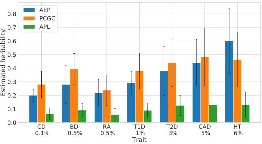
Figure 6: Shown are estimates of heritability (the proportion of liability variance explained by genetic factors) of seven complex disorders from (Wellcome Trust Case Control Consortium et al., 2007). The error bars are the standard deviation multiplied by 1.96, as estimated via jackknife. The disorders are Crohns disease (CD), rheuma-toid arthritis (RA), bipolar disorder (BD), type 1 diabetes (T1D), type 2 diabetes (T2D), coronary artery disease (CAD) and hypertension (HT). The population prevalence of each trait is shown below its name. The estimates of AEP and PCGC are relatively concordant, whereas the APL estimates are significantly down-biased, in agreement with the modeling misspecification simulations.
dimensional vectors encoding the number of minor alleles in SNPs (standardized as in the simulation studies), and θ is a linear scaling factor. We associated sex with a fixed effect and estimated its effect via AGEE. Standard errors were computed via jackknife sampling.
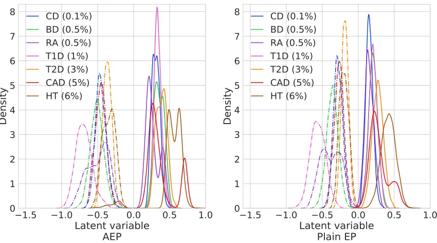
The SNP heritability estimates of the investigated disorders lied in the range 20%-60% (Figure 6). There was a high degree of concordance between PCGC and AEP, whereas the APL estimates were substantially lower, consistent with the simulation studies. To further demonstrate the capabilities of AEP we estimated the posterior distribution of the GP latent variablesgi under both AEP and plain EP, using the standard EP approximation of
1.5
1.0
0.5
0.0
0.5
1.0
Latent variable
AEP
0
1
2
3
4
5
6
7
8
Density
CD (0.1%)
BD (0.5%)
RA (0.5%)
T1D (1%)
T2D (3%)
CAD (5%)
HT (6%)
1.5
1.0
0.5
0.0
0.5
1.0
Latent variable
Plain EP
0
1
2
3
4
5
6
7
8
Density
CD (0.1%)
BD (0.5%)
RA (0.5%)
T1D (1%)
T2D (3%)
CAD (5%)
HT (6%)
Figure 7: Inference of latent variables of complex genetic disorders. Shown is the distri-bution of the posterior mean of latent variables gi provided by AEP (left) and
plain EP (right), estimated via Gaussian kernel density estimation separately for controls (dashed lines) and cases (solid lines). The trait names are the same as in Figure 6, and prevalences are shown in parentheses. Individuals with larger posterior mean estimates carry a greater genetic load of disease-inducing vari-ants. AEP provides a clearer separation between cases and controls by exploiting knowledge about the prevalence and sampling scheme. For both traits, the dis-tribution variance increases with heritability and prevalence. Note that these distributions are not analogous to the ones in Figure 3 because they are based on posterior rather than marginal prior distributions.
5. Discussion
We presented several methods for inference of GP hyperparameters in settings with unit-level ascertainment, and a full-rank, non-sparse covariance structure. This was done by combining the ascertained likelihood framework with GPs and GLMMs, which form the statistical backbone of likelihood based analysis of non-iid data.
the advantage of providing a full probabilistic model with a well-defined likelihood, and it recovers standard EP as a special case under random ascertainment. On the other hand, PCGC has a principled underlying approximation, whereas APL and AEP are less well understood. Hence, the three methods are complementary in terms of their strengths and weaknesses, and we encourage future case-control studies to use multiple methods to gain a deeper understanding of high dimensional dependency structures.
The combination of unit-level ascertainment and a full-rank, non-sparse covariance struc-ture is very common in statistical genetics (Golan et al., 2014), but is often encountered in other scientific domains, such as geostatistics and GP classification (Diggle et al., 1998; Chu et al., 2010; Ziegler et al., 2014; Young et al., 2013). Ascertained sampling is almost inevitable when studying rare phenomena, and the increasing dimensionality of studied data often necessitates the introduction of random rather than fixed effects, which in turn induce full-rank, non-sparse dependency structures. Additionally, it is often more convenient to perform dense sampling in a small number of clusters rather than collecting a large number of clusters (Bellamy et al., 2005; Zhang, 2004; Glidden and Vittinghoff, 2004), leading to non-sparse, full-rank dependency structures at the cluster level. Hence, we expect our work to be applicable in diverse scientific fields.
In this study we extended the well-known EP algorithm (Minka, 2001) to approximate GP likelihood. Another potential approach is MCMC sampling coupled with an integra-tion scheme such as thermodynamic integraintegra-tion (Kuss and Rasmussen, 2005; Nickisch and Rasmussen, 2008; Gelman and Meng, 1998), but in our experience such approaches are too slow and complex for modern sized data sets. In recent years, Bayesian approaches have proven to be potential alternatives to likelihood based approaches in GPs (Ferkingstad and Rue, 2015). However, such approaches can be sensitive to the choice of prior distribution, and require prohibitively computationally expensive MCMC sampling. Several analytical approximations exist, but these are often inaccurate in the presence of binary data (Fong et al., 2010). The potential use of sampling-based approaches for inference in GPs under case-control ascertainment remains to be explored.
In recent years, genetic biobanks with hundreds of thousands of individuals have be-come available (Bycroft et al., 2018). AEP scales cubically with sample size and is thus not scalable to such datasets. GP approximation techniques from the machine learning community, such as mixture-of-experts models (Deisenroth and Ng, 2015), inducing points (Snelson and Ghahramani, 2006; Wilson and Nickisch, 2015; Gardner et al., 2018), random feature expansions (Rahimi and Recht, 2008; Le et al., 2013; Yang et al., 2015) and stochas-tic variational approximations (Hensman et al., 2013; Wilson et al., 2016; Cheng and Boots, 2017), or from the GWAS community (e.g. Loh et al. 2015) can potentially be used to scale up AEP to such large datasets.
models (Zhang and Zimmerman, 2005; Du et al., 2009). Several studies have established the statistical consistency of maximum likelihood estimators for linear mixed models (i.e., GPs with a linear kernel and a normal likelihood) in similar settings using random matrix theory (Bonnet et al., 2015; Jiang et al., 2016b; Dicker and Erdogdu, 2016), but to our knowledge such results have not been derived for GPs with non-normal likelihoods. We conclude that there is a major gap in statistical theory regarding r/m → 0 asymptotics, representing questions of both theoretical and practical importance.
Several topics that remain unexplored in this work are GPs with more advanced kernels, outcome prediction and testing of fixed effects, for which several heuristic methods have been proposed in the statistical genetics literature (Hayeck et al., 2015; Weissbrod et al., 2015; Chen et al., 2016; Jiang et al., 2016a). Extending our approach to handle these topics is a potential avenue for future work.
Acknowledgments
This work was supported by grant 1804/16 from the Israel Science Foundation. This study makes use of data generated by the Wellcome Trust Case Control Consortium. A full list of the investigators who contributed to the generation of the data is available from www.wtccc.org.uk. Funding for the project was provided by the Wellcome Trust under award 076113. We thank Malka Gorfine for fruitful discussions.
Appendix A
Here we describe a fast Taylor expansion-based approximation to APL estimation of GPs with a probit likelihood and a scaling parameter σ2. Denote cov(g
i, gj) = ρσg2, where
gi is the latent variable of unit i and ρ depends on Zi,Zj, and on all the other kernel
hyperparameters. The joint likelihood of each pair of units can be written as:
P(yi =a, yj =b|Xi,Xj,Zi,Zj, si=sj = 1) =
Aab(ρ)
B(ρ) P(si= 1|yi)P(sj = 1|yj), (4)
where Aab(ρ) , P(yi = a, yj = b|Xi,Xj, ρ), B(ρ) , P(si = sj = 1|Xi,Xj, ρ), and
we omitted the hyperparameters θ, β for brevity. Using the law of total probability, we can write: B(ρ) = (s1)2A11(ρ) +s1s0(A10(ρ) +A01(ρ)) + (s0)2A00(ρ), where st =
P(si = 1|yi = t). Next, we explicitly evaluate these quantities at ρ = 0: Aab(0) =
Kia(1−Ki)1−aKjb(1−Kj)1−b, B(0) = s0(1−Ki) +s1Ki
s0(1−Kj) +s1Kj
, where
Ki = P(yi = 1|Xi), and we omitted the dependence on Zi because we assume that
gi ∼ N(0, σ2g) marginally regardless of Zi. The above equations hold because yi, yj and
We next compute the partial derivatives of both expressions with respect to ρatρ= 0. Following (Golan et al., 2014), we have:
d
dρAab(ρ)|ρ=0 =φ(ti)φ(tj)σ
2(−1)a6=b
d
dρB(ρ)|ρ=0 = (s
1)2 d
dρA11(ρ)|ρ=0+ 2s
1s0 d
dρAa6=b(ρ)|ρ=0+ (s
0)2 d
dρA00(ρ)|ρ=0
=φ(ti)φ(tj)σ2 (s1)2+ (s0)2−2s1s0
,
whereφ(·) is the standard normal density, andti= Φ−1(1−K)−XiTβis the liability cutoff
for uniti, with Φ(·) representing the standard normal cumulative density andK being the prevalence of cases in the population.
Finally, we plug in the above expressions into the Taylor expansion of Equation 4 at
ρ= 0, which can be written as follows:
Aab(ρ)
B(ρ) P(si|yi)P(sj|yj) =
A0ab(0)B(0)−B0(0)Aab(0)
B(0)2 ρ+O(ρ 2)
P(si|yi)P(sj|yj).
Appendix B
Here we provide an informal analysis motivating the use of AEP. A formal analysis of AEP is difficult because there are relatively few theoretical guarantees for standard EP (Dehaene and Barthelm´e, 2016, 2018). Instead, we state several assumptions and then provide an informal analysis under these assumptions. Throughout this Appendix, the notation s is a shorthand notation for s1 =. . . =sn = 1, u−i indicates the vector u with theith entry
removed, and we omit the dependence onβ,θ for brevity.
The parametric form of the AEP site approximation
We first demonstrate that in order for AEP to approximate the ascertained likelihood
P(y|X,Z,s) (up to a scaling factor) at its fixed point, the site function ti(gi) needs to
approximately take the following parametric form:
ti(gi)≈
P(yi, si|gi,Xi)
P(si|X,Z,s−i)
. (5)
Note that this is different from the standard EP approximationti(gi)≈P(yi|Xi, gi).
Our derivation requires an additional approximation:
Approximation 1
P(s|X,Z)≈ 1
C(X,Z) Y
i
P(si|X,Z,s−i), for some proportionality factor C(X,Z).
are asymptotically normal with the same mean, the composite likelihood is approximately proportional to the full likelihood around this mean, with the approximation accuracy depending on the ratio between their variances. This ratio depends on the ratio between the diagonal entries of the Fisher and the Godambe information matrices (Varin et al., 2011). Note that if Approximation 1 holds, this implies that it also holds when replacing swiths−j and omittingj from the product. This property will be used in the derivations
below.
Under Equation 5 and Approximation 1, the AEP likelihood R P(g|Z)Q
iti(gi)dg is
approximately proportional to the ascertained likelihoodP(y|X,Z,s):
Z
P(g|Z)Y
i
ti(gi)dg
Equation 5
≈
Z
P(g|Z)Y
i
P(yi, si|gi,Xi)
P(si|X,Z,s−i)
dg
=
Z P(g|Z)Q
iP(si|gi,Xi)
Q
iP(si|X,Z,s−i)
Y
i
P(yi|si, gi,Xi)dg
Approximation 1
≈ C(X,Z)
Z
P(g|Z)P(s|g,X)
P(s|X,Z) P(y|s,g,X)dg
=C(X,Z) Z
P(g|X,Z,s)P(y|s,g,X)dg
=C(X,Z)·P(y|X,Z,s).
The last two equalities use the fact that y, sare conditionally independent of Z given g. We conclude that ifti(gi) approximately takes the form of Equation 5 then the
hyperparam-etersβ,θ which maximize the AEP likelihood are approximately the maximum likelihood estimates.
Derivation of the AEP Step
Here we provide a heuristic motivation for the AEP step procedure. Recall from Section 3.2 that the AEP step consists of finding the unnormalized Gaussianti(gi) that optimizes
the following approximation:
Z
q−i(gi)ti(gi)dgi ≈
R
q−i(gi)P(yi, si|gi,Xi)dgi
R
q−i(gi)P(si|gi,Xi)dgi
, (6)
whereq−i(gi)∝
R
P(g|Z)Q
j6=itj(gj)dg−i, and the optimization is performed by matching
the zeroth, first, and second derivatives of both functions with respect toµ−i.
We first write down the natural analogue of the standard EP step objective for AEP. Ac-cording to Equation 5, this objective finds the unnormalized Gaussianti(gi) that optimizes
the approximation:
Z
q−i(gi)ti(gi)dgi ≈
Z
q−i(gi)
P(yi, si|gi,Xi)
P(si|X,Z,s−i)
dgi. (7)
Unlike standard EP, we cannot minimize the GKL divergence between the functions in the integrals in Equation 7, because this will lead to the same solutionti(gi) as in standard EP
written as q−i(gi)P(yi|gi,Xi)W, where W = P(sP(si|yi)
i|X,Z,s−i) is constant with respect to gi.
Hence, minimizing the GKL divergence will lead to the same approximation as in standard EP, up to the scaling factorW.
Instead of minimizing the GKL divergence, we will approximate the rhs of Equation 7 as follows:
Z
q−i(gi)
P(yi, si|gi,Xi)
P(si|X,Z,s−i)
dgi ≈
R
q−i(gi)P(yi, si|gi,Xi)dgi
R
q−i(gi)P(si|gi,Xi)dgi
. (8)
The AEP step in Equation 6 is obtained by equating the lhs of Equation 7 with the rhs of Equation 8.
It remain to derive Equation 8. Our derivation uses the following assumption:
Assumption 1 Weak dependence between y−i and si conditional on X and on Z:
P(y−i|X,Z,s)≈P(y−i|X,Z,s−i).
The derivation additionally uses the following two approximations, which we derive below by using Equation 5, Approximation 1 and Assumption 1:
Approximation 2 At the fixed point we have: q−i(gi)≈P(gi,X,Z,y−i).
Approximation 3 R
q−i(gi)P(yi,si |gi,Xi)
P(si|X,Z,s−i)dgi ≈P(yi|X,Z,y−i, si).
We complete the derivation of Equation 8 by first using Approximation 3 to approximate the rhs of Equation 7 and the lhs of Equation 8 asP(yi|X,Z,y−i, si), and then using
Approx-imation 2 and the graphical model structure (Figure 2) to approximateP(yi|X,Z,y−i, si)
via q−i(gi) as follows:
P(yi|X,Z,y−i, si) =
P(yi, si|X,Z,y−i)
P(si|X,Z,y−i)
= R
P(gi|X,Z,y−i)P(yi, si|Xi, gi)dgi
R
P(gi|X,Z,y−i)P(si|Xi, gi)dgi
≈
R
q−i(gi)P(yi, si|Xi, gi)dgi
R
q−i(gi)P(si|Xi, gi)dgi
.
This completes the derivation.
Derivation of Approximations 2–3
We now provide heuristic derivations of Approximations 2–3.
Our derivation consists of two stages. First, we define the unnormalized cavity distribution
q−i∗ (gi),
R
P(g|Z)Q
j6=itj(gj)dg−i, and show thatq ∗
−i(gi)≈C(X,Z)·P(gi,y−i|X,Z,s−i):
q−i∗ (gi),
Z
P(g|Z)Y
j6=i
tj(gj)dg−i
Equation 5
≈
Z
P(g|Z)Y
j6=i
P(yj, sj|gj,Xj)
P(sj|X,Z,s−j)
dg−i
Approximation 1
≈ C(X,Z)
Z P(g|Z)
P(s−i|X,Z)
Y
j6=i
P(yj, sj|gi,Xj)dg−i
=C(X,Z) Z
P(g−i|Z)P(gi|g−i,Z)
P(s−i|X,Z)
P(y−i,s−i|g−i,X−i)dg−i
rearrangement
= C(X,Z)
Z P(g
−i|Z)P(s−i|g−i,X−i)
P(s−i|X,Z)
P(y−i,|g−i,s−i,X−i)P(gi|g−i,Z)dg−i
Bayes rule
= C(X,Z) Z
P(g−i|X,Z,s−i)P(y−i,|g−i,s−i,X−i)P(gi|g−i,Z)dg−i
graphical model
= C(X,Z) Z
P(g−i,y−i|X,Z,s−i)P(gi|g−i,X,Z,s−i)dg−i
=C(X,Z) Z
P(g,y−i|X,Z,s−i)dg−i
=C(X,Z)·P(gi,y−i|X,Z,s−i)
Next, we note that since q−i(gi) ,
q∗−i(gi)
R
q−∗i(g
0
i)dg
0
i
is a normalized distribution over gi, we have
q−i(gi)≈P(gi|X,Z,y−i,s−i). Finally, we note thatgi is conditionally independent ofs−i
given y−i due to the graphical model structure, yielding q−i(gi)≈P(gi|X,Z,y−i).
Approximation 3 R q−i(gi)PP((syi,si|gi,Xi)
i|X,Z,s−i)dgi ≈P(yi|X,Z,y−i, si).
First, we invoke Approximation 2 and the graphical model structure to obtain the following approximation:
Z
q−i(gi)
P(yi, si|gi,Xi)
P(si|X,Z,s−i)
dgi
Approximation 2
≈
Z
P(gi|X,Z,y−i)
P(yi, si|gi,Xi)
P(si|X,Z,s−i)
dgi
= Z
P(gi|X,Z)P(y−i|gi,X,Z)
P(y−i|X,Z)
P(yi, si|gi,Xi)
P(si|X,Z,s−i)
dgi
=
Z P(g
i|X,Z)P(y−i|gi,X,Z)
P(y−i|X,Z)
P(yi|gi,X,Z,y−i)P(si|yi)
P(si|X,Z,s−i)
dgi
= R
P(gi|X,Z)P(y|gi,X,Z)dgiP(si|yi)
P(y−i|X,Z)P(si|X,Z,s−i)
= P(y|X,Z)P(si|yi)
P(y−i|X,Z)P(si|X,Z,s−i)
Next, we multiply the rhs of Equation 9 by P(s−i|y−i)P(s−i|X,Z)
P(s−i|y−i)P(s−i|X,Z) and invoke Assumption 1:
P(y|X,Z)P(si|yi)
P(y−i|X,Z)P(si|X,Z,s−i)
P(s−i|y−i)P(s−i|X,Z)
P(s−i|y−i)P(s−i|X,Z)
= P(y|X,Z)
P(y−i|X,Z)
P(s|y)P(s−i|X,Z)
P(s|X,Z)P(s−i|y−i)
= P(y
|X,Z)PP(s(|sX|y,Z))
P(y−i|X,Z)PP((ss−i|y−i)
−i|X,Z)
= P(y|X,Z,s)
P(y−i|X,Z,s−i)
= P(y−i|X,Z,s)P(yi|X,Z,y−i,s)
P(y−i|X,Z,s−i)
Assumption 1
≈ P(y−i|X,Z,s−i)P(yi|X,Z,y−i,s)
P(y−i|X,Z,s−i)
=P(yi|X,Z,y−i,s)
=P(yi|X,Z,y−i, si)
Appendix C
Here we describe our novel development of ascertained generalized estimating equations (AGEE). GEEs are extensions of generalized linear models that can estimate fixed effects while accounting for dependencies without requiring a probabilistic model (Liang and Zeger, 1993). GEEs require a correct specification of the mean of the outcome conditional on the features, µi = E[yi|Xi,β], and a (possibly misspecified) working covariance matrix of
the outcomes, denoted as Ω θΩ and parameterized by θΩ. Given these, β is estimated by solving the estimating equation ∂∂µβΩ θΩ−1(y−µ(β)) = 0. GEEs yield consistent estimates ofβand its sampling variance even if the covariance structure is misspecified and is non-sparse (Xie and Yang, 2003).
GEEs can naturally be adapted to case-control settings by using the ascertained con-ditional mean function E[yi|Xi, si = 1,β] = P(yi= 1|Xi, si = 1,β). We now show how
the GEE fixed effect estimates can be plugged into GPs. In the general case it is not pos-sible to reconcile fixed effect estimates of GEEs and GPs, because GEEs assume that the conditional mean of the outcome is affected only by the fixed effects, whereas GPs assume that it is affected by both the fixed effects and the GP latent variable. Fortunately, the probit likelihood provides a convenient way to reconcile the two approaches. DenoteβGEE and βGP as the vectors of fixed effects used by GEE and GP, respectively. When using a probit likelihood, the GEE conditional mean is given by Φ(XiTβGEE), where Φ(·) is the standard normal cumulative density. In contrast, the GP conditional mean is given by Φ
XT
iβGP
(var(gi)+1)1/2
. If var(gi) is constant for every unit i (which corresponds to a constant
value on the diagonal of the covariance matrix ofg), the two approaches can be reconciled by definingβGP=βGEE(var(gi) + 1)1/2.In practice, the diagonal of the covariance matrix
ofgis often exactly or almost exactly constant, which enables exploiting the above relation. Therefore, we can use the GEE estimates in a GP by settingβGP=βGEE(var(gi) + 1)1/2.
References
Scarlett L. Bellamy, Yi Li, Xihong Lin, and Louise M. Ryan. Quantifying PQL bias in estimating cluster-level covariate effects in generalized linear mixed models for group-randomized trials. Stat. Sin., 15(4):1015–1032, 2005.
Benjamin M. Bolker, Mollie E. Brooks, Connie J. Clark, Shane W. Geange, John R. Poulsen, M. Henry H. Stevens, and Jada-Simone S. White. Generalized linear mixed models: a practical guide for ecology and evolution. Trends Ecol. Evol., 24(3):127–35, 2009.
Anna Bonnet, Elisabeth Gassiat, and Cline Lvy-Leduc. Heritability estimation in high dimensional sparse linear mixed models. Electron. J. Stat., 9(2):2099–2129, 2015.
Norman E. Breslow. Statistics in epidemiology: the case-control study. J. Am. Stat. Assoc., 91(433):14–28, 1996.
Norman E. Breslow and David G. Clayton. Approximate inference in generalized linear mixed models. J. Am. Stat. Assoc., 88(421):9–25, 1993.
Paul R. Burton, Katrina J. Tiller, Lyle C. Gurrin, William OCM Cookson, A. William Musk, and Lyle J. Palmer. Genetic variance components analysis for binary phenotypes using generalized linear mixed models (GLMMs) and Gibbs sampling. Genet. Epidemiol., 17(2):118–140, 1999.
Clare Bycroft, Colin Freeman, Desislava Petkova, Gavin Band, Lloyd T Elliott, Kevin Sharp, Allan Motyer, Damjan Vukcevic, Olivier Delaneau, Jared OConnell, et al. The uk biobank resource with deep phenotyping and genomic data. Nature, 562(7726):203, 2018.
Han Chen, Chaolong Wang, Matthew P. Conomos, Adrienne M. Stilp, Zilin Li, Tamar Sofer, Adam A. Szpiro, Wei Chen, John M. Brehm, Juan C. Celed´on, et al. Control for population structure and relatedness for binary traits in genetic association studies via logistic mixed models. Am. J. Hum. Genet., 98(4):653–666, 2016.
Ching-An Cheng and Byron Boots. Variational inference for Gaussian process models with linear complexity. In Advances in Neural Information Processing Systems, pages 5184– 5194, 2017.
Carlton Chu, Peter Bandettini, John Ashburner, Andre Marquand, and Stefan Kloeppel. Classification of neurodegenerative diseases using Gaussian process classification with automatic feature determination. In Workshop on brain decoding: Pattern recognition challenges in neuroimaging (WBD), 2010, pages 17–20. IEEE, 2010.
David R. Cox and Nancy Reid. A note on pseudolikelihood constructed from marginal densities. Biometrika, 91(3):729–737, 2004.
Guillaume Dehaene and Simon Barthelm´e. Bounding errors of Expectation-Propagation. In Advances in Neural Information Processing Systems, pages 244–252, 2016.
Guillaume Dehaene and Simon Barthelm´e. Expectation Propagation in the large data limit.
Marc Deisenroth and Jun Wei Ng. Distributed Gaussian processes. In International Con-ference on Machine Learning, volume 37, pages 1481–1490, 07–09 Jul 2015.
Everett R. Dempster and I. Michael Lerner. Heritability of threshold characters. Genetics, 35(2):212–36, 1950.
Lee H. Dicker and Murat A. Erdogdu. Maximum likelihood for variance estimation in high-dimensional linear models. In International Conference on Artificial Intelligence and Statistics, pages 159–167, 2016.
Peter J. Diggle, Jonathan A. Tawn, and Rana Moyeed. Model-based geostatistics. J. R. Stat. Soc. C, 47(3):299–350, 1998.
Juan Du, Hao Zhang, and Vidyadhar Mandrekar. Fixed-domain asymptotic properties of tapered maximum likelihood estimators. Ann. Stat., 37(6A):3330–3361, 2009.
Georg B. Ehret, Patricia B. Munroe, Kenneth M. Rice, Murielle Bochud, Andrew D. John-son, Daniel I. Chasman, Albert V. Smith, Martin D. Tobin, Germaine C. Verwoert, Shih-Jen Hwang, et al. Genetic variants in novel pathways influence blood pressure and cardiovascular disease risk. Nature, 478(7367):103–109, 2011.
Michael P. Epstein, Xihong Lin, and Michael Boehnke. Ascertainment-adjusted parameter estimates revisited. Am. J. Hum. Genet., 70(4):886–95, 2002.
Ludwig Fahrmeir and Gerhard Tutz. Multivariate Statistical Modelling Based on General-ized Linear Models. Springer Series in Statistics. Springer New York, Berlin, 2nd edition, 2001. ISBN 978-0-387-95187-4.
Egil Ferkingstad and H˚avard Rue. Improving the INLA approach for approximate Bayesian inference for latent Gaussian models. Electron. J. Stat., 9(2):2706–2731, 2015.
Youyi Fong, H˚avard Rue, and Jon Wakefield. Bayesian inference for generalized linear mixed models. Biostatistics, 11(3):397–412, 2010.
Jacob Gardner, Geoff Pleiss, Ruihan Wu, Kilian Weinberger, and Andrew Wilson. Prod-uct kernel interpolation for scalable Gaussian processes. In International Conference on Artificial Intelligence and Statistics, volume 84, pages 1407–1416, 2018.
Andrew Gelman and Xiao-Li Meng. Simulating normalizing constants: From importance sampling to bridge sampling to path sampling. Stat. Sci., 13(2):163–185, 1998.
David V. Glidden and Kung-Yee Liang. Ascertainment adjustment in complex diseases.
Genet. Epidemiol., 23(3):201–208, 2002.
David V. Glidden and Eric Vittinghoff. Modelling clustered survival data from multicentre clinical trials. Stat. Med., 23(3):369–88, 2004.
David Golan and Saharon Rosset. Effective genetic-risk prediction using mixed models.
David Golan, Eric Lander, and Saharon Rosset. Measuring missing heritability: Inferring the contribution of common variants. Proc. Natl. Acad. Sci. USA, 111(49):E5272–81, 2014.
Tristan J. Hayeck, Noah A. Zaitlen, Po-Ru Loh, Bjarni Vilhjalmsson, Samuela Pollack, Alexander Gusev, Jian Yang, Guo-Bo Chen, Michael E. Goddard, Peter M. Visscher, et al. Mixed model with correction for case-control ascertainment increases association power. Am. J. Hum. Genet., 96(5):720–730, 2015.
Patrick J Heagerty and Subhash R Lele. A composite likelihood approach to binary spatial data. J. Am. Stat. Assoc., 93(443):1099–1111, 1998.
Leonhard Held, Isabel Natrio, Sarah Elaine Fenton, H˚avard Rue, and Nikolaus Becker. Towards joint disease mapping. Stat. Methods Med. Res., 14(1):61–82, 2005.
James Hensman, Nicolo Fusi, and Neil D Lawrence. Gaussian processes for big data. In
Conference on Uncertainty in Artificial Intelligence, 2013.
James Hensman, Alexander G Matthews, Maurizio Filippone, and Zoubin Ghahramani. MCMC for variationally sparse Gaussian processes. In Advances in Neural Information Processing Systems, pages 1648–1656, 2015.
David A Hsieh, Charles F Manski, and Daniel McFadden. Estimation of response probabil-ities from augmented retrospective observations. J. Am. Stat. Assoc., 80(391):651–662, 1985.
Duo Jiang, Joelle Mbatchou, and Mary Sara McPeek. Retrospective association analysis of binary traits: overcoming some limitations of the additive polygenic model. Hum. Hered., 80(4):187–195, 2015.
Duo Jiang, Sheng Zhong, and Mary Sara McPeek. Retrospective binary-trait association test elucidates genetic architecture of Crohn disease. Am. J. Hum. Genet., 98(2):243–255, 2016a.
Jiming Jiang, Cong Li, Debashis Paul, Can Yang, and Hongyu Zhao. On high-dimensional misspecified mixed model analysis in genome-wide association study. Ann. Stat., 44(5): 2127–2160, 2016b.
Julia E Kelsall and Peter J. Diggle. Spatial variation in risk of disease: a nonparametric binary regression approach. J. Royal Stat. Soc. C, 47(4):559–573, 1998.
H. K¨onig. Eigenvalue Distribution of Compact Operators. Operator Theory: Advances and Applications. Birkh¨auser Basel, 2013. ISBN 9783034862783.
Malte Kuss and Carl Edward Rasmussen. Assessing approximate inference for binary Gaus-sian process classification. J. Mach. Learn. Res., 6:1679–1704, 2005.
Quoc Le, Tamas Sarlos, and Alexander Smola. Fastfood - computing Hilbert space expan-sions in loglinear time. InInternational Conference on Machine Learning, pages 244–252, 2013.
Sang Hong Lee, Naomi R. Wray, Michael E. Goddard, and Peter M. Visscher. Estimat-ing missEstimat-ing heritability for disease from genome-wide association studies. Am. J. Hum. Genet., 88(3):294–305, 2011.
Kung-Yee Liang and Scott L Zeger. Longitudinal data analysis using generalized linear models. Biometrika, 73(1):13–22, 1986.
Kung-Yee Liang and Scott L Zeger. Regression analysis for correlated data. Annu. Rev. Public Health, 14(1):43–68, 1993.
Po-Ru Loh, Gaurav Bhatia, Alexander Gusev, Hilary K Finucane, Brendan K Bulik-Sullivan, Samuela J Pollack, Teresa R de Candia, Sang Hong Lee, Naomi R Wray, Ken-neth S Kendler, et al. Contrasting genetic architectures of schizophrenia and other com-plex diseases using fast variance-components analysis. Nat. Genet., 47(12):1385–1392, 2015.
Charles F. Manski. Alternative estimators and sample designs for discrete choice analysis. The MIT Press, 1981.
Charles E McCulloch, Shayle R Searle, and John M Neuhaus. Generalized, Linear, and Mixed Models. Wiley Series in Probability and Statistics, 2nd edition, 2008. ISBN 0-470-01181-5.
Thomas P Minka. Expectation Propagation for approximate Bayesian inference. In Uncer-tainty in Artificial Intelligence, pages 362–369, 2001. ISBN 1-55860-800-1.
J. M. Neuhaus, Alastair J. Scott, Chris J. Wild, Y. Jiang, C. E. McCulloch, and R. Boylan. Likelihood-based analysis of longitudinal data from outcome-related sampling designs.
Biometrics, 70(1):44–52, 2014.
John M. Neuhaus and Nicholas P. Jewell. The effect of retrospective sampling on binary regression models for clustered data. Biometrics, 46(4):977–990, 1990.
John M. Neuhaus, Alastair H. Scott, and Chris J. Wild. The analysis of retrospective family studies. Biometrika, 89(1):23–37, 2002.
John M. Neuhaus, Alastair J. Scott, and Chris J. Wild. Family-specific approaches to the analysis of case-control family data. Biometrics, 62(2):488–94, 2006.
Yukinori Okada, Di Wu, Gosia Trynka, Towfique Raj, Chikashi Terao, Katsunori Ikari, Yuta Kochi, Koichiro Ohmura, Akari Suzuki, Shinji Yoshida, et al. Genetics of rheumatoid arthritis contributes to biology and drug discovery. Nature, 506(7488):376–381, 2014.
Manfred Opper and C´edric Archambeau. The variational Gaussian approximation revisited.
Neural Comput, 21(3):786–92, 2009.
Manfred Opper and Ole Winther. Gaussian processes for classification: Mean-field algo-rithms. Neural Comput, 12(11):2655–2684, 2000.
Dirk Pfeiffer. Spatial Analysis in Epidemiology. Oxford University Press, 2008.
Alkes L. Price, Chris C. A. Spencer, and Peter Donnelly. Progress and promise in under-standing the genetic basis of common diseases. Proc Biol Sci, 282(1821), 2015.
Qibin Qi, Adrienne M Stilp, Tamar Sofer, Jee-Young Moon, Bertha Hidalgo, Adam A Szpiro, Tao Wang, Maggie CY Ng, Xiuqing Guo, Yii-Der Ida Chen, et al. Genetics of type 2 diabetes in US Hispanic/Latino individuals: results from the Hispanic Community Health Study/Study of Latinos (HCHS/SOL). Diabetes, 66(5):1419–1425, 2017.
Yuan Alan Qi, Thomas P Minka, Rosalind W Picard, and Zoubin Ghahramani. Predic-tive automatic relevance determination by Expectation Propagation. In International Conference on Machine Learning, page 85, 2004.
Sophia Rabe-Hesketh, Anders Skrondal, and Andrew Pickles. Generalized multilevel struc-tural equation modeling. Psychometrika, 69(2):167–190, 2004.
Sophia Rabe-Hesketh, Anders Skrondal, and Andrew Pickles. Maximum likelihood estima-tion of limited and discrete dependent variable models with nested random effects. J. Econom., 128(2):301–323, 2005.
Ali Rahimi and Benjamin Recht. Random features for large-scale kernel machines. In
Advances in Neural Information Processing Systems, pages 1177–1184, 2008.
Carl E. Rasmussen and Christopher K. I. Williams. Gaussian Processes for Machine Learn-ing. The MIT Press, 2006. ISBN 978-0-262-18253-9.
Stephen W. Raudenbush, Meng-Li Yang, and Matheos Yosef. Maximum likelihood for generalized linear models with nested random effects via high-order, multivariate Laplace approximation. J. Comp. Graph. Stat., 9(1):141–157, 2000.
Didier Renard, Geert Molenberghs, and Helena Geys. A pairwise likelihood approach to estimation in multilevel probit models. Comput. Stat. Data Anal., 44(4):649–667, 2004.
Stephen Sawcer, Garrett Hellenthal, Matti Pirinen, Chris CA Spencer, Nikolaos A Pat-sopoulos, Loukas Moutsianas, Alexander Dilthey, Zhan Su, Colin Freeman, Sarah E Hunt, et al. Genetic risk and a primary role for cell-mediated immune mechanisms in multiple sclerosis. Nature, 476(7359):214–9, 2011.
Alastair J Scott and Chris J Wild. Fitting regression models to case-control data by maxi-mum likelihood. Biometrika, 84(1):57–71, 1997.
Alastair J. Scott and Chris J. Wild. Maximum likelihood for generalised case-control studies.
J. Stat. Plan. Inference, 96(1):3–27, 2001.
Matthias Seeger. Low rank updates for the cholesky decomposition. Technical report, 2004.
Matthias Seeger. Expectation propagation for exponential families. Technical report, 2005.
Zhenming Shun and Peter McCullagh. Laplace approximation of high dimensional integrals.
J. R. Stat. Soc. B, 57(4):749–760, 1995.
Edward Snelson and Zoubin Ghahramani. Sparse Gaussian processes using pseudo-inputs. In Advances in Neural Information Processing Systems, pages 1257–1264, 2006.
Luke Tierney and Joseph B Kadane. Accurate approximations for posterior moments and marginal densities. J. Am. Stat. Assoc., 81(393):82–86, 1986.
Cristiano Varin, Nancy Reid, and David Firth. An overview of composite likelihood meth-ods. Stat. Sin., 21(1):5–42, 2011.
Aki Vehtari, Tommi Mononen, Ville Tolvanen, Tuomas Sivula, and Ole Winther. Bayesian leave-one-out cross-validation approximations for Gaussian latent variable models. J. Mach. Learn. Res., 17(1):3581–3618, 2016.
Peter M. Visscher, Naomi R. Wray, Qian Zhang, Pamela Sklar, Mark I. McCarthy, Matthew A. Brown, and Jian Yang. 10 years of GWAS discovery: biology, function, and translation. Am. J. Hum. Genet., 101(1):5–22, 2017.
Omer Weissbrod, Christoph Lippert, Dan Geiger, and David Heckerman. Accurate liability estimation improves power in ascertained case-control studies. Nat. Methods, 12(4):332–4, 2015.
Omer Weissbrod, Dan Geiger, and Saharon Rosset. Multikernel linear mixed models for complex phenotype prediction. Genome Res., 26(7):969–79, 2016.
Omer Weissbrod, Jonathan Flint, and Saharon Rosset. Estimating SNP-based heritability and genetic correlation in case-control studies directly and with summary statistics. Am. J. Hum. Genet., 103(1):89–99, 2018.