Formulation of Finite Element Method for 1-D
Poisson Equation
Mrs. Pallavi P. Chopade#, Dr. Prabha S. Rastogi*
#
Research Scholar, *Department of Mathematics Shri. J. J. T. University, Jhunjhunu, Rajasthan, India
Abstract -This paper focuses on the use of solving electrostatic one-dimension Poisson differential equation boundary-value problem. Sample problems that introduce the finite element methods are presented here and evaluated with analytical and numerical approaches. These approaches are developed in MATLAB and their solutions are compared and verified. Error analysis is also presented in this paper where the numerical error is compute dusing two different definitions namely the percent error and the error based on the L2 norm. this numerical error is reduced by increasing in number of elements.
Keywords: Boundary-value problems, Differential equation, Electrostatics, Finite Element Method, Poisson’s equation.
I. INTRODUCTION
Differential equations have wider applications in various fields of engineering and science disciplines. Generally, these are used to model variations of any physical quantity (temperature, pressure, displacement, stress, etc) with respect to time ‘t’ or space having coordinates (x,y,z).Based on the involvement of ordinary or partial derivatives, differential equations can be classified as an ordinary differential equation or partial differential equation. They can be also classified as linear/non-linear.
The Poisson’s equation, Fourier equation, heat equation and Poisson’s equation are among the most prominent PDEs that undergraduate engineering students will encounter. The usual practice is to introduce the student to the analytical solution of these equations via the method of separation of variables. Under the assumption of linearity, the method naturally leads to the formulation of solutions as Fourier series expansions.
The numerical solution of differential equations has become one of powerful activity during the last sixty years or so, primarily due to advances in computer technology and the introduction of numerical computing applications like MATLAB, Mathematica, Maple which in turn has led to improvements in the numerical methods that are used. As a result, many scientific and engineering problems that involve linear and nonlinear singular ordinary differential equations and partial differential equations that were previously unsolved can now be resolved by using suitable numerical methods.
The three-dimensional Poisson equation for a function (𝑥, 𝑦, 𝑧) , describing the electrostatic potential when unpaired electric charge is present is given as [8], [9],
𝜕2 𝑉
𝜕𝑥2 +
𝜕2 𝑉
𝜕𝑦2 +
𝜕2 𝑉
𝜕𝑧2 = −
𝜌 𝜀0
𝑜𝑟 ∇2𝑉 = −𝜌
𝜀0
#1
where 𝑥, 𝑦 and 𝑧 are the independent variables, 𝑉is the unknown function, and ∇2is the Laplacian operator.The
solution of equation to be found is supplemented by initial and/or boundary conditions.
Consider the variation of potential in one of the three independent variables. The Poisson’s equation becomes an ordinary derivative and reduces to one dimensional as[2], [3], [5],
𝑑2𝑉
𝑑𝑥2= −
𝜌
𝜀0, 𝑜𝑟 𝑑2𝑉
𝑑𝑦2= −
𝜌
𝜀0, 𝑜𝑟 𝑑2𝑉
𝑑𝑧2 = −
𝜌 𝜀0#2
with initial and final points as boundary conditions.
In this paper finite element method is presented in the context of problems arising in electrostatics particularly one-dimensionPoisson equation with Dirichlet boundary conditions, to understand the concept of finite element method in engineering field [6].
II. FINITE ELEMENT SOLUTION TO ONE DIMENSIONAL DIFFERENTIAL EQUATION
The basic concept used in finite element method is representation of domain into smaller subdomains known as finite elements. The distribution of the primary unknown quantity inside these elements is interpolated based on the values of the edge, if vector elements are provided or based on values of nodes, if nodal elements are used. The shape function or interpolations used to distribute these elements must be a complete set of polynomials. The accuracy of the solution provided depends upon the order of the polynomials used. This solution is obtained after solving set of linear equations by one of the methods used in algebra.The linear equations are formed by converting the governing differential equation and associated boundary conditions to an integrodifferential formulation either by use of weighted residual method (Galerkin approach) or by minimizing a function[1], [4], [7].
The key steps involved in applying the Galerkin method to obtain the FEM solution of a boundary value problem are-
Step 1: Domain discretization using finite elements
Step2: Chose appropriate interpolation function or shape function or basis function
Step3: Obtain corresponding linear equation for single element by applying the boundary conditions. Step 4: Formulate the Global matrix system of equations through assembly of all elements and then
apply the Dirichlet boundary conditions.
Step5: Solve the linear equation using one of the linear algebra techniques such as Cramer’s rule,etc. Step 6: Post process the obtained results.
Here, a one-dimension electrostatic boundary value problem is studied whose solution is obtained using finite element method.The reason to choose one dimensional problem is to understand the steps involved in solving rather than dealing with extensive mathematical derivations and geometrical complications. Further, it can be extended to two-dimensional and three-dimensional problems.The accuracy and effectiveness of the FEM is evaluated by comparing the numerical result with analytical results [1], [10].
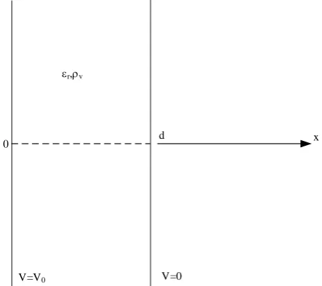
Problem definition: Consider a two infinite in extent parallel conducting plates that are positioned normal to the x-axis and separated by a distance𝑑, as shown in Figure1. One plate is kept a fixed potential𝑉 = 2and these condplate is maintained at𝑉 = 0(ground). The region between the plates is filled with anon magnetic medium having a dielectric constant 𝜀𝑟and a uniform electron volume charge density𝜌𝑣 = −𝜌0.Obtain the electric (orelectrostatic)potential in the region between the two parallel plates.
x d
V=V0 V=0
0
er,rv
Fig. 1: Electrostatic Numerical showing boundary condition
A)Analytical Solution:
The potential distribution at any point between the two plates is governedby Poisson’s equation as,
∇ 𝜀𝑟∇𝑉 = −
𝜌𝑣 𝜀0
#3
which is subject to set of boundary conditions,
𝑉 0 = 𝑉0
and
For a simple nonmagnetic medium (homogeneous, linear and isotropic), Poisson’s equation in one dimension can be suitably written as,
𝑑2𝑉
𝑑𝑥2 =
𝜌0 𝜀𝑟𝜀0
#4
where 𝜌𝑣was replaced by −𝜌0. Integrating equation 4 twice, the equation of potential is,
𝑉 𝑥 = 𝜌0 2𝜀𝑟𝜀0𝑥
2+ 𝑐
1𝑥 + 𝑐0#5
where 𝑐1 and 𝑐0 are constants to be determined from set of given Dirichletconditions. Thus, imposing the two boundary conditions in equation 5, the analytical solution takes the form,
𝑉 𝑥 = 𝜌0 2𝜀𝑟𝜀0
𝑥2− 𝜌0𝑑
2𝜀𝑟𝜀0
+𝑉0
𝑑 𝑥 + 𝑉0#6
B) FEM Solution
This is one of the powerful numerical method to solve the given problem. Our main objective is to compute the electric potential distribution between two parallel plates separated by a distance 𝑑 and positioned normal to the x-axis.
The leftmost plate is maintained at a constant potential𝑉0 whereas the rightmost plate is grounded. The region between the plates is characterizedby a dielectric constant 𝜀𝑟 and a uniform electron charge density −𝜌0.
For a finite element simulation and comparison of the numerical solution with the exact analytical solution, following parameters are considered,
𝜀𝑟= 1
𝑉0= 2𝑉 𝑑 = 8 𝑐𝑚 𝜌0= 10−8 𝐶/𝑚3
Consider, the domain between plates is equally divided into four linear finite elements as shown in figure 2.
4
3
2 1
2
1 3 4 5
x1=0 x2=2 x3=4 x4=6 x5=8
x(cm)
Fig. 2: Discretization of given domain in four elements
All the elements in the domain are characterized by the same length 𝑙𝑒and the same dielectric constant 𝜀
𝑟𝑒. Thus,
the element coefficient matrix 𝐾𝑒is given by,
𝐾𝑒= 8.85 ∗ 10−12
2 ∗ 10−12
+1 −1
−1 +1 = 4.425 ∗ 10
−10 +1 −1
−1 +1 #7
where 𝜀𝑒 = 𝜀
𝑟𝑒𝜀0= 8.85 ∗ 10−12 𝐹/𝑚 and 𝑙𝑒 = 2 ∗ 10−2 𝑚.The element right hand side vector 𝑓𝑒becomes,
𝑓𝑒= −2 ∗ 10
−2∗ 10−8
2
1
1 = −10−10 1 1 #8
The contribution of the right-hand-side vector 𝑑𝑒 to the global right-hand-side vector,is zero for all nodes except
for the two end nodes of the domain. However, at these two end nodes, Dirichlet boundary conditions must be imposed and, therefore, the contribution by vector 𝑑𝑒is effectively discarded. Thus, the global matrix system for
the finite elements mesh becomes,
4.425 ∗ 10−10
1 −1 0 0 0 −1 2 −1 0 0 0 −1 2 −1 0 0 0 −1 2 −1 0 0 0 −1 1
𝑉1 𝑉2 𝑉3 𝑉4 𝑉5 = −10−10 1 2 2 2 1 #9
Evaluating further we get,
1 −1 0 0 0 −1 2 −1 0 0 0 −1 2 −1 0 0 0 −1 2 −1 0 0 0 −1 1
𝑉1 𝑉2 𝑉3 𝑉4 𝑉5 = −0.2259887 −0.4519774 −0.4519774 −0.4519774 −0.2259887 #10
𝑏𝑖 = 𝑏𝑖−𝑘𝑖 𝑉0#11
Thus, the matrix gets reduced to,
2 −1 0 0 −1 2 −1 0 0 −1 2 −1 0 0 −1 1
𝑉2 𝑉3 𝑉4 𝑉5 = 1.5480226 −0.4519774 −0.4519774 −0.2259887 #12
The secondary condition 𝑉 = 0 at node 5 is imposed by eliminating the entire last row of matrix system and last column of coefficient matrix.
Thus, the final global matrix becomes,
2 −1 0 −1 2 −1
0 −1 2 𝑉2 𝑉3 𝑉4 = 1.5480226 −0.4519774 −0.4519774 #13
This global matric can be solved using Cramer’s rule giving the values of 𝑉2, 𝑉3 𝑎𝑛𝑑 𝑉4i.e. the electric potential at three interior nodes of finite element domain.
∴ 𝑉2= 0.8220339, 𝑉3= 0.0960451 𝑎𝑛𝑑 𝑉4= −0.1779661#14
The electric potential at intermediate points requires the use of the interpolation or shape functions employed for each finite element for plotting of graph. For the given numerical, linear interpolation functions were used and, thus, the numerical solution at intermediate points inside an element is given by,
𝑉 𝜉 = 𝑉1𝑒𝑁
1 𝜉 + 𝑉2𝑒𝑁2 𝜉 #15
where
𝑁1 𝜉 =
1 − 𝜉 2 #16 𝑁2 𝜉 =
1 + 𝜉 2 #17
and
𝜉 =2 𝑥 − 𝑥1
𝑒
𝑥2𝑒− 𝑥 1𝑒
− 1#18
Substituting these values equations 16 and 17 becomes,
𝑁1 𝑥 =
𝑥2𝑒− 𝑥
𝑥2𝑒− 𝑥1𝑒#19
and
𝑁2 𝑥 = 𝑥 − 𝑥1
𝑒
𝑥2𝑒− 𝑥 1𝑒
#20
Hence,
𝑉 𝜉 = 𝑉1𝑒
𝑥2𝑒− 𝑥
𝑥2𝑒− 𝑥 1𝑒
+ 𝑉2𝑒
𝑥 − 𝑥1𝑒
𝑥2𝑒− 𝑥 1𝑒
#21
where 𝑉1𝑒and 𝑉
2𝑒are the values of the electric potential at the two end nodes of the element.
C)FEM Algorithm in MATLAB
The FEM Algorithm developed in MATLAB is discussed as
Step1: Define the parameters by initialising it.
Step2: Discretise the domain by number of elements.
Step 3: Calculate the element coefficient matrix.
Step 4: Based on assembly process, calculate the global matrix system for finite element mesh by imposing the boundary conditions.
Step 5: Post process the result.
Results
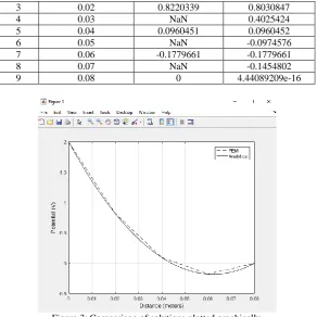
The electric potential for the four-element mesh over the complete domain is evaluated using the developed algorithm. The results obtained are shown in table 1 and is graphically plotted in figure 3.
TABLE 1:COMPARISON OF RESULTS
Sr. No. x
(Distance in meters)
Potential (V) using FEM Solution
Potential (V) using Analytical Solution
1 0 2 2
3 0.02 0.8220339 0.8030847
4 0.03 NaN 0.4025424
5 0.04 0.0960451 0.0960452
6 0.05 NaN -0.0974576
7 0.06 -0.1779661 -0.1779661
8 0.07 NaN -0.1454802
9 0.08 0 4.44089209e-16
Figure 3: Comparison of solutions plotted graphically
From the Figure 3, the electric potential at the nodes of the finite element mesh matches perfectly the analytical solution, whereas at intermediate evaluation points there is a deviation between the two solutions. The reason for this deviation stems from the fact that the numerical solution at intermediate points is an interpolation of the nodal values using linear shape functions. An acceptable representation of the numerical error between the finite element solution and the analytical solution is defined as the area bounded by the two curves, which are depicted in Figure 3, as compared to the total area under the curve described by the exact solution. The numerical error is given by,
𝑒𝑟𝑟𝑜𝑟 % = 1 𝐴𝑎𝑛
𝐴𝑎𝑛 𝑒 − 𝐴𝑓𝑒𝑚 𝑒
𝑁𝑒
𝑒=1
∗ 100%#22
The L2 norm that represents the distance between two methods, is computed to quantify the numerical
discrepancy between the finite element solution and analytical solution is given as,
𝐿2𝑛𝑜𝑟𝑚 = 𝑉𝑎𝑛 − 𝑉𝑓𝑒𝑚
2= 𝑉𝑎𝑛 𝑒 − 𝑉
𝑓𝑒𝑚 𝑒 2𝑑𝑥 Ω𝑒
𝑁𝑒
𝑒=1
1 2
#23
The numerical error as function of number of linear elements is shown in Table II. TABLE II:NUMERICAL ERROR FUNCTION
Sr. No. Number of linear elements Percentage error (Numerical) Error based on L2 norm
1 4 9.4786729 0.0116700
2 8 2.3696682 0.0029175
3 12 1.0531858 0.0012966
4 16 0.5924170 7.2937539e-04
5 20 0.3791469 4.6680025e-04
6 24 0.2632964 3.2416684e-04
From Table II it is observed that as the number of linear elements is doubling, both the error reduces at the same rate (by a factor of four). Thus, increase in the number of elements the numerical solution converges to analytical solution.
III. CONCLUSION
deviation is because of interpolation of nodal values which uses linear shape functions. A n increase in the number of elements the numerical solution approaches to analytical solution. Further, using higher order interpolation functions, the finite element solution will be accurately represented within discretized domain substantially reducing the numerical error.
REFERENCES
[1]. Lonngren, K.E., Savov, S.V. and Jost, R.J., 2007.Fundamentals of Electromagnetics with MATLAB. Scitech publishing.
[2]. Papanikos, G. and Gousidou-Koutita, M.C., 2015. A Computational Study with Finite Element Method and Finite Difference Method for 2D Elliptic PartialDifferential Equations.Applied Mathematics,6(12), p.2104.
[3]. Chaudhari, T.U. and Patel, D.M., 2015. Finite Element Solution of Poisson’s equation in a homogeneous medium.
[4]. Brenner, S. and Scott, R., 2007.The mathematical theory of finite element methods(Vol. 15). Springer Science & Business Media.
[5]. Sharma, N., Formulation of Finite Element Method for 1D and 2D Poisson Equation.
[6]. Agbezuge, L., 2006. Finite Element Solution of the Poisson equation with Dirichlet Boundary Conditions in a rectangular domain. [7]. Jain, M.K., 2003.Numerical methods for scientific and engineering computation. New Age International.
[8]. Rao, N., 2008.Fundamentals of Electromagnetics for Engineering. Pearson Education India.
[9]. Sadiku, M.N., 2011.Numerical techniques in electromagnetics with MATLAB. CRC press.