A New And Efficient Proposed Approach For Optimizing The Initial Basic Feasible Solution Of A Linear Transportation Problem

ISSN: 2231-5373

http://www.ijmttjournal.org

Page 104

A New And Efficient Proposed Approach For

Optimizing The Initial Basic Feasible Solution

Of A Linear Transportation Problem

Opara Jude1, Oruh Ben Ifeanyichukwu2, Ihekuna Stephen, O.3, Okenwe Idochi4

1

Department of Statistics, Michael Okpara University of Agriculture Umudike P.M.B. 7267, Umuahia Abia State, Nigeria

2

Department of Mathematics, Michael Okpara University of Agriculture, Umudike P.M.B. 7267, Umuahia, Abia State, Nigeria

3

Department of Statistics, Imo State University, PMB 2000, Owerri Nigeria

4

Department of Statistics, School of Applied Sciences, Ken Saro Wiwa Polytechnic PMB 20, Bori, Rivers State Nigeria

Abstract

In this research, a new approach (Loop Product Difference) for optimizing the initial basic feasible solution of a balanced transportation problem is proposed. The proposed technique has been tested and proven efficient by solving several number of cost minimizing transportation problems and it was discovered that the method gives the same result as that of optimal solution obtained by using MODI/Stepping stone methods. Conclusively, it can be said that proposed technique is easy to adopt and close to optimality if employed with the Inverse Coefficient of Variation Method as an improved technique of obtaining Initial Basic Feasible Solution.

Keywords: Transportation Problem, Inverse Coefficient of Variation Method, Initial Basic Feasible Solution, Optimal Solution, Loop Product Difference.

INTRODUCTION

Transportation Problem (TP) is linked with supply and demand of commodities transported from several sources to the different destinations. The destinations where commodities arrive are regarded as the demand while the sources from which one needs to transport are regarded as the supply. Transportation problem is popular in operations research for its real life wide application. This is a special kind of network optimization problems which deals with the determination of a minimum-cost schedule for transporting a single commodity from a number of sources (warehouses) to a number of destinations (markets). This class of problem which is basically a linear programming problem can be extended to some practical applications such as inventory control, staff assignment, job scheduling, cash flow etc. The optimal solution to the classical transportation problem requires the determination of a number of units of commodities to be transported from each origin to various destinations, satisfying source availability and destination demands so that the total cost of transportation is minimum. The available amounts at the supply points and the amounts required at the demand points are the parameters of the transportation problem (Deshabrata et al, 2013).

ISSN: 2231-5373

http://www.ijmttjournal.org

Page 105

There are basically three stages for the solution procedure for the transportation problem:

Stage 1: Mathematical formulation of the transportation problem, Stage 2: Finding an initial basic feasible solution,

Stage 3: Optimize the initial basic feasible solution which is obtained in Stage 2.

Our focus in this study is on stage 3: to propose a new and easy technique for optimizing the initial basic feasible solution.

Related Literature Review

Abul and Mosharraf (2018) carried out a research on an Innovative Algorithmic Approach for Solving Profit Maximization Problems. In their study, a new algorithmic technique was developed to tackle the profit maximization problems using transportation algorithm of Transportation Problem (TP) which included three basic parts; first converting the maximization problem into the minimization problem, second formatting the Total Opportunity Table (TOT) from the converted Transportation Table (TT), and last allocations of profits using the Row Average Total Opportunity Value (RATOV) and Column Average Total Opportunity Value (CATOV). The algorithm considered the average of the cell values of the TOT along each row identified as RATOV and the average of the cell values of the TOT along each column identified as CATOV. Allocations of profits are started in the cell along the row or column which has the highest RATOVs or CATOVs. The study concluded that the Initial Basic Feasible Solution (IBFS) obtained by the method is better than some other familiar methods which were discussed in the study with the three different examples, even though the results or outcomes of the algorithm were optimal or near optimal solutions.

Amaravathy et al (2018) worked on Optimal Solution of OFSTF, MDMA Methods with Existing Methods Comparison. In their study, a different approach OFSTF (Origin, First, Second, Third, and Fourth quadrants) Method was applied for obtaining a feasible solution for transportation problems directly. The proposed method was a unique, it gave always feasible (may be optimal for some extant) solution without disturbance of degeneracy condition. The method involved minimum iterations to reach optimality. A numerical example was solved to check the validity of the proposed method and degeneracy problem was also discussed.

In the present work we experiment with a new transportation technique for optimal solution with less calculation, using Inverse Coefficient of Variation Method (ICVM) as a technique for obtaining initial feasible solution to a transportation problem.

Model Formulation of a Linear Transportation Problem

The formulation of the transportation model employs double – subscripted variables of the form xij. Thus, the

general formulation of the transportation problem with supply (sp), demand (d), n sources and m destinations, is given by

Minimize





 

m

1 j

ij ij n

1 i

x

C

Subject to (sp)i sp i 1,2,3, ,n

n

1 i

  





m

j

d

d

j m

j

,

,

3

,

2

,

1

1











The general formulation of the transportation problem reveals that m supply constraints and n demand constraints translate into m + n total constraints.

ISSN: 2231-5373

http://www.ijmttjournal.org

Page 106

The algorithm for the method for determining the optimal solution to transportation problem of the proposed approach is stated as follows:

► Determine the initial basic feasible solution by using Northwest Corner Method (NWCM), Least Cost Method (LCM), Vogel’s Approximation Method (VAM), Row Minimum Method (RMM), Column Minimum Method (CMM), Allocation Table Method (ATM) or Inverse Coefficient of Variation Method (ICVM).

In this study, the Inverse Coefficient of Variation Method (ICVM) gives a better result (close to optimal) according to Opara et al (2017). Hence, it was employed to obtain the initial basic feasible solution in this study.

Test for Optimality using the Proposed Technique (Loop Product Difference)

Basically, there are two well known methods of obtaining optimal solution indirectly (obtaining first the initial basic feasible solution), which are MODI method and Stepping Stone method. Hence, the new algorithm for obtaining the optimal solution of the linear transportation problem indirectly is discussed below.

Step 1: Form a closed path for the entire non basic cell. The closed path has the following properties: ►It starts and ends in the identified cell.

►It consists of a series of alternate horizontal and vertical connected lines only (no diagonals). ►It can be traced anticlockwise or clockwise.

►All other corners of the path lie in the allocated cells only. ► The path may skip over any number of allocated or vacant cells.

► There will always be one and only one closed path, which may be traced.

It should be noted that the closed path has even number of corners (4, 6, 8, 10, etc) and any allocated cell can be considered only once. The shape of a closed path may or may not be square or rectangular; it may have a peculiar configuration and the lines may even cross over.

● Having formed the closed path, mark the identified empty cell as positive and each occupied cell at the corners of the path alternately –ve, +ve, –ve, +ve and so on.

Step 2: For each non basic cell, determine

P

_ts



C

_ts

C

_mc



C

_mc

C

_nmc



C

_tqand if

P

_ts



0

, stop. Otherwise obtain

P

ts



min



C

ts

C

mc



C

mc

C

nmc





C

tq and go to step 3, where

C

ts is the cost of the leaving variable in

the closed path with a positive sign,

C

_mcis the smallest cost in the closed path with a positive sign,

C

_mc is the

smallest cost in the closed path with a negative sign, and

C

_nmcis the next smallest cost in the closed path with a negative sign.

Step 3: The non basic variable say

C

_tqenters the basis since

C

_tq



0

. Allocate

x

_tq





, (where



is found as in the linear transportation case) in the concerned closed loop, which when modified by the

x

_tq





value will keep

i

a

and

j

b

values unchanged. Determine the leaving variable say

Btk

x

, where

Btk

x

is the basic variable which

turns to zero while making the modification, and

x

_tq





becomes the new basic variable, and go to Step 1.

Numerical Problems using the Proposed Technique

ISSN: 2231-5373

http://www.ijmttjournal.org

Page 107

Illustration of the New Algorithm

Example 1

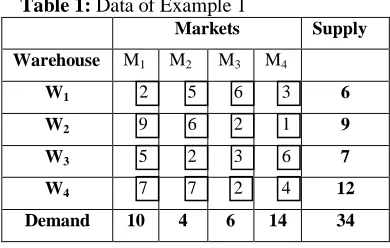
Consider a Transportation problem with four markets and four warehouses. The market demands are 10, 4, 6, and 14 while the warehouse capacities are 6, 9, 7, and 12. The cell entries represent unit cost of transportation, and the table is shown in Table 1.

Table 1: Data of Example 1

Markets Supply

Warehouse M1 M2 M3 M4

W1 2 5 6 3 6

W2 9 6 2 1 9

W3 5 2 3 6 7

W4 7 7 2 4 12

Demand 10 4 6 14 34

Solution

The initial basic feasible solution using Inverse Coefficient of Variation Method (ICVM) is summarized in Table 2.

Table 2: Initial Basic Feasible Solution Table of Example 1

Hence, the total transportation cost is 6(2) + 9(1) + 3(5) + 4(2) + 1(7) + 6(2) + 5(4) = N83.

Test for Optimality using the Proposed Technique (Loop Product Difference)

Steps 1 and 2

For cell (1, 2), the loop can be expressed as:

2 (6)

5

6 3

9 6

2

1 (9) 5

(3)

2 (4)

3

6

7 (1)

7 2

(6)

4 (5)

nmc mc mc

ts

C

C

C

C

_



_{ }



ts

P

;

P

₁₂



C

₁₂

C

₃₁



C

₁₁

C

₃₂



5

(

5

)



2

(

2

)



21

Markets

Warehouses M1 M2 M3 M4

W1 2 (6)

5 6 3

W2 9 6 2 1 (9)

W3 5 (3)

2 (4)

3 6

W4 7 (1)

7 2

(6)

4 (5)

–

– +

ISSN: 2231-5373

http://www.ijmttjournal.org

Page 108

For cell (1, 3), the loop can be expressed as:

2 (6)

5

6 3

9 6

2 1 (9) 5 (3) 2 (4) 3 6 7 (1)

7 2

(6) 4 (5) nmc mc mc

ts

C

C

C

C

_



_{ }



ts

P

;

P

₁₃



C

₁₃

C

₄₁



C

₁₁

C

₄₃



6

(

7

)



2

(

2

)



38

For cell (1, 4), the loop can be expressed as:

2 (6)

5

6 3

9 6

2 1 (9) 5 (3) 2 (4) 3 6 7 (1)

7 2

(6)

4 (5)

;

P

₁₄



C

₁₄

C

₄₁



C

₁₁

C

₄₄



3

(

7

)



2

(

4

)



13

For cell (2, 1), the loop can be expressed as:

2 (6)

5

6 3

9 6

2 1 (9) 5 (3) 2 (4) 3 6 7 (1)

7 2

(6)

4 (5)

;

P

₂₁



C

₂₁

C

₄₄



C

₂₄

C

₄₁



9

(

4

)



1

(

7

)



29

For cell (2, 2), the loop can be expressed as:

2 (6)

5

6 3

9 6

2 1 (9) 5 (3) 2 (4) 3 6 7 (1)

7 2

(6)

4 (5)

;

P

22



C

22

C

44



C

24

C

32



6

(

4

)



1

(

2

)



22

nmc mc mc

ts

C

C

C

C

_



_{ }



ts

P

nmc mc mc

ts

C

C

C

C

_



_{ }



ts

P

nmc mc mc

ts

C

C

C

C

_



_{ }

ISSN: 2231-5373

http://www.ijmttjournal.org

Page 109

For cell (2, 3), the loop can be expressed as:

2 (6)

5

6 3

9 6

2 1 (9) 5 (3) 2 (4) 3 6 7 (1)

7 2

(6)

4 (5)

;

P

₂₃



C

₂₃

C

₄₄



C

₂₄

C

₄₃



2

(

4

)



1

(

2

)



6

For cell (3, 3), the loop can be expressed as:

2 (6)

5

6 3

9 6

2 1 (9) 5 (3) 2 (4) 3 6 7 (1)

7 2

(6)

4 (5)

;

P

33



C

33

C

41



C

43

C

31



3

(

7

)



2

(

5

)



11

For cell (3, 4), the loop can be expressed as: 2

(6)

5

6 3

9 6

2 1 (9) 5 (3) 2 (4) 3 6 7 (1)

7 2

(6)

4 (5)

;

P

₃₄



C

₃₄

C

₄₁



C

₄₄

C

₃₁



6

(

7

)



4

(

5

)



22

For cell (4, 4), the loop can be expressed as:

2 (6)

5

6 3

9 6

2 1 (9) 5 (3) 2 (4) 3 6 7 (1)

7 2

(6)

4 (5)

;

P

₄₄



C

₄₄

C

₃₁



C

₃₂

C

₄₁



7

(

5

)



2

(

7

)



21

nmc mc mc

ts

C

C

C

C

_



_{ }



ts

P

nmc mc mc

ts

C

C

C

C

_



_{ }



ts

P

nmc mc mc

ts

C

C

C

C

_



_{ }



ts

P

– – + + – + + – – + + – – + – + nmc mc mc

ts

C

C

C

C

_



_{ }

ISSN: 2231-5373

http://www.ijmttjournal.org

Page 110

Since none of the product difference

(P

_ts

)

is negative, we stop; the present feasible solution is optimal. Hence, the optimal solution is

6

X₁₁ ,X₂₄ 9, X₃₁3, X₃₂4, X₄₁1, X₄₃6, X₄₄ 5 and the minimum cost for this transportation problem is 6

             

2 9135 42 17 62 54 N83.

Example 2

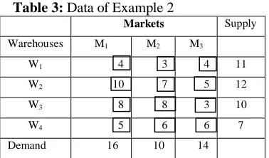
Consider the transportation problem with three markets and four warehouses. The market demands are 16, 10, 14, while the warehouse capacities are 11, 12, 10, 7. The unit cost of transportation is as given in Table 3.

Table 3: Data of Example 2

Markets Supply

Warehouses M1 M2 M3

W1 4 3 4 11

W2 10 7 5 12

W3 8 8 3 10

W4 5 6 6 7

Demand 16 10 14

The initial basic feasible solution using Inverse Coefficient of Variation Method (ICVM) is summarized in Table 4.

Table 4: Initial Basic Feasible Solution Table of Example 1

Markets

Warehouses M1 M2 M3

W1 4

(11)

3 4

W2 10 7

(8)

5 (4)

W3 8 8 3

(10)

W4 5

(5)

6 (2)

6

Total transportation cost = 11(4) + 8(7) + 4(5) + 10(3) + 5(5) + 2(6) = 187

Test for Optimality using the Proposed Technique

Steps 1 and 2

For cell (1, 2), the loop can be expressed as:

4 (11)

3

4

10 7

(8)

5 (4) 8

8 3

(10) 5

(5)

6 (2)

6

;

P

₁₂



C

₁₂

C

₄₁



C

₁₁

C

₄₂



3

(

5

)



4

(

6

)





9

+ –

– +

nmc mc mc

ts

C

C

C

C

_



_{ }

ISSN: 2231-5373

http://www.ijmttjournal.org

Page 111

For cell (1, 3), the loop can be expressed as:

4 (11)

3

4

10 7

(8)

5 (4) 8

8 3

(10) 5 (5) 6 (2) 6

;

P

₁₃



C

₁₃

C

₄₁



C

₁₁

C

₂₃



4

(

5

)



4

(

5

)



0

For cell (2, 1), the loop can be expressed as:

4 (11)

3

4

10 7

(8)

5 (4) 8

8 3

(10) 5 (5) 6 (2) 6

;

P

₂₁



C

₂₁

C

₄₂



C

₄₁

C

₂₂



10

(

6

)



5

(

7

)



25

For cell (3, 1), the loop can be expressed as:

4 (11)

3

4

10 7

(8)

5 (4) 8

8 3

(10) 5 (5) 6 (2) 6

;

P

₃₁



C

₃₁

C

₂₃



C

₃₃

C

₄₁



8

(

5

)



3

(

5

)



25

For cell (3, 2), the loop can be expressed as:

4 (11)

3

4

10 7

(8)

5 (4) 8

8 3

(10) 5 (5) 6 (2) 6

;

P

₃₂



C

₃₂

C

₂₃



C

₃₃

C

₂₂



8

(

5

)



3

(

7

)



19

nmc mc mc

ts

C

C

C

C

_



_{ }



ts

P

nmc mc mc

ts

C

C

C

C

_



_{ }



ts

P

nmc mc mc

ts

C

C

C

C

_



_{ }



ts

P

– – + + + – – – + + – – + + + – – – + + nmc mc mc

ts

C

C

C

C

_



_{ }

ISSN: 2231-5373

http://www.ijmttjournal.org

Page 112

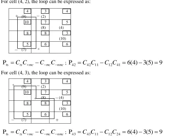
For cell (4, 3), the loop can be expressed as:

4 (11)

3

4

10 7

(8)

5 (4) 8

8 3

(10) 5

(5)

6 (2)

6

;

P

₄₃



C

₄₃

C

₂₂



C

₂₃

C

₄₂



6

(

7

)



5

(

6

)



12

Step 3:





9

min

C

_ts

C

_mc



C

_mc

C

_nmc



P

₁₂





It is obvious that the presence of negative value for the empty cell signifies non optimality; hence we readjust. Therefore

x

₁₂ should enter the basis since it is the most negative empty cell cost, after adjusting the values

x

42 left

the basic.

Markets Supply

Warehouses M1 M2 M3

W1 4

11

3

(-9)

4

(0) 11

W2 10

(25)

7

8

5

4

12

W3 8

(25)

8

(19) 3

10

10

W4 5

5

6

2

6

(12) 7

Demand 16 10 14

The basic variable with the least value among the corners having negative sign in the loop is the leaving variable. Hence,

x

₄₂ with the least value of 2 is the leaving variable. Thus, we increase the corners with + sign by 2, and reduce the ones with – sign by 2. The adjusted tableau becomes:

Markets Supply

Warehouses M1 M2 M3

W1 4

9

3

2

4 11

W2 10 7

8

5

4

12

W3 8 8 3

10

10

W4 5

7

6 6 7

Demand 16 10 14

At the end of this stage of iteration, the basic feasible solution is

nmc mc mc

ts

C

C

C

C

_



_{ }



ts

P

+

– +

–

+

+ –

ISSN: 2231-5373

http://www.ijmttjournal.org

Page 113

9

11



x

,

x

₁₂



2

,

x

₂₂



8

,

x

₂₃



4

,

x

₃₃



10

,

x

₄₁



7

We then go back to Steps 1 and 2

For cell (1, 3), the loop can be expressed as:

4 (9)

3 (2)

4

10 7

(8)

5 (4) 8

8 3

(10) 5 (7) 6 6

;

P

₁₃



C

₁₃

C

₂₂



C

₁₂

C

₂₃



4

(

7

)



3

(

5

)



13

For cell (2, 1), the loop can be expressed as:

4 (9)

3 (2)

4

10 7

(8)

5 (4) 8

8 3

(10) 5 (7) 6 6

;

P

₂₁



C

₂₁

C

₁₂



C

₁₁

C

₂₂



10

(

3

)



4

(

7

)



2

For cell (3, 1), the loop can be expressed as:

4 (9)

3 (2)

4

10 7

(8)

5 (4) 8

8 3

(10) 5 (7) 6 6

;

P

₃₁



C

₃₁

C

₁₂



C

₃₃

C

₁₁



8

(

3

)



3

(

4

)



12

For cell (3, 2), the loop can be expressed as:

4 (9)

3 (2)

4

10 7

(8)

5 (4) 8

8 3

(10) 5 (7) 6 6

;

P

32



C

32

C

23



C

33

C

22



8

(

5

)



3

(

7

)



19

nmc mc mc

ts

C

C

C

C

_



_{ }



ts

P

nmc mc mc

ts

C

C

C

C

_



_{ }



ts

P

nmc mc mc

ts

C

C

C

C

_



_{ }



ts

P

nmc mc mc

ts

C

C

C

C

_



_{ }

ISSN: 2231-5373

http://www.ijmttjournal.org

Page 114

For cell (4, 2), the loop can be expressed as:

4 (9)

3 (2)

4

10 7

(8)

5 (4) 8

8 3

(10) 5

(7)

6

6

;

P

42



C

42

C

11



C

12

C

41



6

(

4

)



3

(

5

)



9

For cell (4, 3), the loop can be expressed as:

4 (9)

3 (2)

4

10 7

(8)

5 (4) 8

8 3

(10) 5

(7)

6

6

;

P

₄₃



C

₄₃

C

₁₁



C

₁₂

C

₂₄



6

(

4

)



3

(

5

)



9

Since none of the product difference

(P

_ts

)

is negative, we stop; the present feasible solution is optimal. Hence, the optimal solution is

9

11



x

,

x

₁₂



2

,

x

₂₂



8

,

x

₂₃



4

,

x

₃₃



10

,

x

₄₁



7

and the minimum cost for this transportation problem is

9

       

4



2

3



8

7



4

5



10

   

3



7

5



183

.

The remaining five examples shall be presented in their last tableau without illustration.

Example 3

Dangote Flour Mills Plc is a manufacturing company located in Calabar. The company produces Bread Flour (BF), Confectionery Flour (CF), Penny Semolina (PS) and Wheat Offals (WO). These products are supplied to thefollowing states (locations) Bayelsa, Anambra, Rivers, Kano, Abia, Enugu, AkwaIbom etc. For the purpose ofthis study, only four (4) of these demand points shall be considered; Enugu, Akwa-Ibom, Anambra and Rivers. Theestimated supply capacities of the four products, the demand requirements at the four sites (states) and the transportation cost per bag of each product are given in Table 5.

Table 5: Data of Example 3 Enugu Akwa

-Ibom

Anambra Rivers Supply

BF 45 52 63 57 15500

CF 58 48 56 54 12000

PS 52 55 62 58 14400

WO 65 48 44 54 11600

Demand 12600 12500 13000 15400 53500

The initial basic feasible solution using Inverse Coefficient of Variation Method (ICVM) is summarized in Table 6.

nmc mc mc

ts

C

C

C

C

_



_{ }



ts

P

nmc mc mc

ts

C

C

C

C

_



_{ }



ts

P

+

–

–

+

+ –

–

ISSN: 2231-5373

http://www.ijmttjournal.org

Page 115

Table 6: Initial Basic Feasible Solution Table of Example 3 Enugu

Akwa-Ibom

Anambra Rivers

BF 45

(12600)

52 (2900)

63 57

CF 58 48

(9600)

56 (1400)

54 (1000)

PS 52 55 62 58

(14400)

WO 65 48 44

(11600)

54

Hence, the total transportation cost is 12600(45) + 2900(52) + 9600(48) + 1400(56) + 1000(54) + 14400(58) + 11600(44) = 2,656,600.

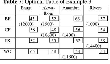
The optimal table using the proposed technique is summarized in Table 7

Table 7: Optimal Table of Example 3 Enugu

Akwa-Ibom

Anambra Rivers

BF 45

(12600)

52 (1900)

63 57 (1000)

CF 58 48

(10600)

56 (1400)

54

PS 52 55 62 58

(14400)

WO 65 48 44

(11600)

54

The solution is optimal at iteration two and the optimal solution is

x

₁₁



12600

,

x

₁₂



1900

,

x

₂₂



10600

,

1400

23



x

,

x

₃₄



14400

,

x

₄₃



11600

and the minimum cost for this transportation problem is



12600



52



1900



57



1000



48



10600



56



1400



58



14400



44



11600



2

,

655

,

600

45















.

Example 4

Consider a Transportation problem with four markets and three warehouses. The market demands are 10, 6, 8, and 12 while the warehouse capacities are 12, 14, and 10.The cell entries represent unit cost of transportation, and the table is shown in Table 8.

Table 8: Data of Example 4

Markets

Warehouses M1 M2 M3 M4 Supply

W1 5 7 9 6 12

W2 6 7 10 5 14

W3 7 6 8 1 10

Demand 10 6 8 12 36

The initial basic feasible solution using Inverse Coefficient of Variation Method (ICVM) is summarized in Table 9.

Table 9: Initial Basic Feasible Solution Table of Example 4

Markets

Warehouses M1 M2 M3 M4

W1 5

(10)

7 9

(2)

6

W2 6 7

(6)

10 (6)

5 (2)

W3 7 6 8 1

(10)

ISSN: 2231-5373

http://www.ijmttjournal.org

Page 116

Example 5

A company manufactures motor cars and it has three factories F1, F2 and F3whose weekly production capacities are

300, 400 and 500 pieces of cars respectively. The company supplies motor cars to its four showrooms located at D1,

D2, D3 and D4 whose weekly demands are 250, 350, 400 and 200 pieces of cars respectively. The transportation

costs per piece of motor cars are given in the transportation Table 10. Find out the schedule of shifting of motor cars from factories to showrooms with minimum cost:

Table 10: Data of Example 5

Showrooms Factories D1 D2 D3 D4

F1 3 1 7 4 300

F2 2 6 5 9 400

F3 8 3 3 2 500

Demand 250 350 400 200

The initial basic feasible solution using Inverse Coefficient of Variation Method (ICVM) is summarized in Table 11.

Table 11: Initial Basic Feasible Solution Table of Example 5

Showrooms Factories D1 D2 D3 D4

F1 3 1

(300)

7 4

F2 2

(250)

6 5

(150) 9

F3 8 3

(50)

3 (250)

2 (200)

Total transportation cost = 300(1) + 250(2) + 150(5) + 50(3) + 250(3) + 200(2) = 2850. The present initial basic feasible solution is optimal using the proposed technique.

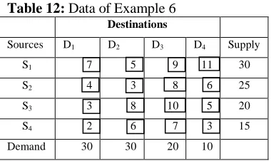
Example 6

Consider the following transportation problem (Transportation Table 12) involving four sources and four destinations. The cell entries represent the cost of transportation per unit. Obtain an initial basic feasible solution.

Table 12: Data of Example 6

Destinations

Sources D1 D2 D3 D4 Supply

S1 7 5 9 11 30

S2 4 3 8 6 25

S3 3 8 10 5 20

S4 2 6 7 3 15

Demand 30 30 20 10

The initial basic feasible solution using Inverse Coefficient of Variation Method (ICVM) is summarized in Table 13.

Table 13: Initial Basic Feasible Solution Table of Example 6

Destinations

Sources D1 D2 D3 D4

S1 7

(5)

5 (5)

9 (20)

11

S2 4 3

(25)

8 6

S3 3

(20)

ISSN: 2231-5373

http://www.ijmttjournal.org

Page 117

S4 2

(5)

6 7 3

(10)

Total transportation cost = 5(7) + 5(5) + 20(9) + 25(3) + 20(3) + 5(2) + 10(3) = 415. The optimal solution table using the proposed technique is summarized in Table 14

Table 14: Optimal Table of Example 6

Destinations

Sources D1 D2 D3 D4

S1 7 5

(10)

9 (20)

11

S2 4

(5)

3 (20)

8 6

S3 3

(20)

8 10 5

S4 2

(5)

6 7 3

(10)

The solution is optimal at iteration two and the optimal solution is

x

₁₂



10

,

x

13



20

,

x

21



5

,

x

22



20

,

20

31



x

,

x

₄₁



5

,

x

₄₄



10

and the minimum cost for this transportation problem is

 

5

20

   

9

5

4

20

 

3

20

   

3

5

2

10

 

3

410

10















.

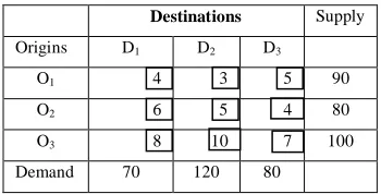
Example 7

Consider the following transportation problem (Transportation Table 15) involving three origins and three destinations. The cell entries represent the cost of transportation per unit. Obtain an initial basic feasible solution.

Table 15: Data of Example 7

Destinations Supply Origins D1 D2 D3

O1 4 3 5 90

O2 6 5 4 80

O3 8 10 7 100

Demand 70 120 80

The initial basic feasible solution using Inverse Coefficient of Variation Method (ICVM) is summarized in Table 16.

Table 16: Initial Basic Feasible Solution Table of Example 7

Destinations

Origins D1 D2 D3

O1 4 3

(90)

5

O2 6 5

(30)

4 (50)

O3 8

(70)

10 7

(30)

The transportation cost = 90(3) + 30(5) + 50(4) + 70(8) + 30(7) = 1390. The present initial basic feasible solution is optimal using the proposed technique.

CONCLUSION

ISSN: 2231-5373

http://www.ijmttjournal.org

Page 118

adopt and close to optimality if employed with the Inverse Coefficient of Variation Method as an improved technique of obtaining Initial Basic Feasible Solution.

REFERENCES

[1] Abul, K. A., and Mosharraf, H. (2018). An Innovative Algorithmic Approach for Solving Profit Maximization Problems. Mathemati cs Letters. Vol. 4, No. 1, 2018, pp. 1-5. doi: 10.11648/j.ml. 20180401.11

[2] Amaravathy, A., Thiagarajan, K. and Vimala, S. (2018). Optimal Solution of OFSTF, MDMA Methods with Existing Methods Comparison. International Journal of Pure and Applied Mathematics. Volume 119 No. 10 2018, 989-1000.

[3] Deshabrata, R. M., Sankar, K. R., Mahendra, P.B. (2013). Multi-choice stochastic transportation problem involving extreme value distribution. 37(4).

[4] Gurupada, M., Sankar, K. R., and José, L. V. (2016). Multi-Objective Transportation Problem With Cost Reliability Under Uncertain Environment. International Journal of Computational Intelligence Systems, 9(5).

[5] Hakim, M.A. (2012). An Alternative Method to Find Initial Basic Feasible Solution of a Transportation Problem, Annals of Pure and Applied Mathematics, Vol. 1, No. 2, 2012, 203-209.

[6] Opara, J., Oruh, B. I., Iheagwara, A. I., and Esemokumo, P. A. (2017). A New and Efficient Proposed Approach to Find Initial Basic Feasible Solution of a Transportation Problem. American Journal of Applied Mathematics and Statistics, 2017, Vol. 5, No. 2. [7] Roy, S.K. (2016). Transportation Problem with Multi-choice Cost and Demand and Stochastic Supply J. Operations Research of

China (2016) 4(2), 193-204, DOI 10.1007/s40305-016-0125-3

[8] Roy, S.K., Maity, G. & Weber, G.W. (2017). Multi-objective two-stage grey transportation problem using utility function with goals Cent Eur. J. Oper. Res. (2017) 25: 417.

[9] Sankar, K.R., Gurupada, M., Gerhard, W.W., Sirma, Z.A.G. (2016). Conic Scalarization Approach to solve choice Multi-objective Transportation Problem with interval goal. Annals of Operations Research · August 2016 DOI: 10.1007/s10479-016-2283-4. [10] Sudipta, M. & Sankar, K. R. (2014). Solving Single-Sink, Fixed-Charge, Multi-Objective, Multi-Index Stochastic Transportation