Statistical Analysis and Parameter Selection for Mapper
Mathieu Carri`ere [email protected]
Inria Saclay
91120 Palaiseau, France
Bertrand Michel [email protected]
LMJL UMR 6629– Ecole Centrale Nantes 44322 Nantes, France
Steve Oudot [email protected]
Inria Saclay
91120 Palaiseau, France
Editor:Kevin Murphy and Bernhard Sch¨olkopf
Abstract
In this article, we study the question of the statistical convergence of the 1-dimensional Mapper to its continuous analogue, the Reeb graph. We show that the Mapper is an optimal estimator of the Reeb graph, which gives, as a byproduct, a method to automatically tune its parameters and compute confidence regions on its topological features, such as its loops and flares. This allows to circumvent the issue of testing a large grid of parameters and keeping the most stable ones in the brute-force setting, which is widely used in visualization, clustering and feature selection with the Mapper.
Keywords: Topological Data Analysis, Mapper, Parameter Selection, Confidence Re-gions, Extended Persistence
1. Introduction
In statistical learning, a large class of problems can be categorized into supervised or un-supervised problems. For un-supervised learning problems, an output quantity Y must be predicted or explained from the input measures X. On the contrary, for unsupervised problems there is no output quantity Y to predict and the aim is to explain and model the underlying structure or distribution in the data. In a sense, unsupervised learning can be thought of as extracting features from the data, assuming that the latter come with unstructured noise. Many methods in data sciences can be qualified as unsupervised meth-ods, among the most popular examples are association methmeth-ods, clustering methmeth-ods, linear and non linear dimension reduction methods and matrix factorization to cite a few (see for instance Chapter 14 in Friedman et al. (2001)). Topological Data Analysis (TDA) has emerged in the recent years as a new field whose aim is to uncover, understand and exploit the topological and geometric structure underlying complex and possibly high-dimensional data. Most of TDA methods can thus be qualified as unsupervised. In this paper, we study a recent TDA algorithm called Mapper which was first introduced in Singh et al. (2007).
Starting from a point cloudXnsampled from a metric space X, the idea of the Mapper
is to study the topology of the sublevel sets of a function f : Xn → R defined on the
c
point cloud1. The functionf is called afilter functionand it has to be chosen by the user. The Mapper construction depends on the choice of a cover I of the image of f by open sets. Pulling back I through f gives an open cover of the domain Xn. It is then refined
into a connected cover by splitting each element into its various clusters using a clustering algorithm whose choice is left to the user. Then, the Mapper is defined as the nerve of the connected cover, having one vertex per element, one edge per pair of intersecting elements, and more generally, one k-simplex per non-empty (k+ 1)-fold intersection. It can also be seen as a discrete approximation of its continuous counterpart called theReeb graph, which was originally introduced in Reeb (1946).
In practice, the Mapper has two major applications. The first one is data visualization and clustering. Indeed, when the cover I is minimal in terms of cardinality, i.e. no more than two cover elements can intersect at once, the Mapper provides a visualization of the data in the form of a graph whose topology reflects that of the data. As such, it brings additional information to the usual clustering algorithms by identifying flares and loops
that outline potentially remarkable subpopulations in the various clusters. See e.g. Yao et al. (2009); Lum et al. (2013); Sarikonda et al. (2014); Hinks et al. (2015) for examples of applications. The second application of Mapper is about feature selection. Indeed, each feature of the data can be evaluated on its ability to discriminate the interesting subpopulations mentioned above (flares, loops) from the rest of the data, using for instance Kolmogorov-Smirnov tests. See e.g. Lum et al. (2013); Nielson et al. (2015); Rucco et al. (2015) for examples of applications.
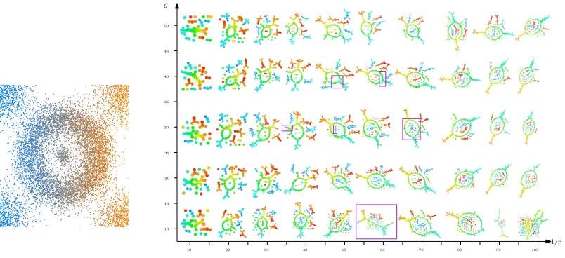
Unsupervised methods generally depend on parameters that need to be chosen by the user, such as the number of selected dimensions for dimension reduction methods or the number of clusters for clustering methods. Contrarily to supervised problems, it can be very difficult to evaluate the output of unsupervised methods and thus to select parameters. Re-garding Mapper, the only answer proposed in the literature consists in selecting parameters in a range of values for which the Mapper seems to be stable—see for instance Nielson et al. (2015). But with non trivial data sets, it is not easy to tune Mapper this way. The problem is illustrated for instance in Figure 1 on a data set that we study further in Sec-tion 5. More generally, we believe that such an approach is not satisfactory since it does not provide statistical guarantees on the inferred Mapper. This major drawback of Mapper is an important obstacle to its use in exploratory data analysis.
Contributions. Our main goal in this article is to provide a statistical method to tune the parameters of the Mapper automatically in various settings (Equations (8), (9) and (10)) by computing its rate of convergence (Propositions 11 and 13 and Corollary 14) to its continu-ous counterpart called the Reeb graph, avoiding the computational cost of testing millions of candidates and selecting the most stable ones in the brute-force setting of many practi-tioners. We also provide methods to assess stability, rates of convergence and confidence regions (Proposition 15) for the topological features of the Mapper. We believe that this set of methods open the way to an accessible and intuitive utilization of Mapper for non expert researchers in applied topology.
1. The Mapper was originally defined more generally for functions with values inRd, with arbitraryd >0.
g
1/r
10 20 30 40 50 60 70 80 90 100
10 20 30 40 50
15 25 35 45
Figure 1: A collection of Mappers computed with various parameters. Left: crater data set. Right: outputs of Mapper with various parameters. One can see that for some Mappers (the ones with purple squares), topological features suddenly appear and disappear. These are discretization artifacts, that we overcome in this article by appropriately tuning the parameters.
Related work. Theoretical properties of Reeb graphs and Mappers have been the topic of several recent articles. Reeb graphs are now well understood and have been used in a wide range of applications. Algorithms for their computation have been proposed, as well as studies of their homology groups, like in Dey et al. (2017), and metrics for their comparison, such as the functional distortion distance of Bauer et al. (2014), the interleaving distance
of de Silva et al. (2016) and the edit distance of di Fabio and Landi (2016). We refer the interested reader to the survey Biasotti et al. (2008) and to the introductions of Bauer et al. (2014) and Bauer et al. (2015) for a comprehensive list of references.
Concerning the Mapper, Babu (2013) characterized the Mapper with coarsened levelset zigzag persistence modules and showed that, as the lengths of the intervals in the coverI go to zero uniformly, the Mapper of a real-valued function converges to the Reeb graph in the bottleneck distance (defined in Section 2.2). Similarly, Munch and Wang (2016) recently characterized the Mapper with constructible cosheaves and showed the same type of con-vergence for the Mapper in the interleaving distance. Their result holds in the general case of vector-valued functions. However, in both approaches, the quantification of convergence is not precise enough to enable parameter selection.
Map-per. In this article, the authors provide a way to go from the input space to the Mapper using small perturbations. We build on this precise relation between the input space and its Mapper to show that the Mapper is itself a measurable construction. In Carri`ere and Oudot (2017b), the authors also show that the topological structure of the Mapper can actually be predicted from the cover I by looking at appropriate signatures that take the form of extended persistence diagrams. In this article, we use this observation, together with an approximation inequality, to show that the Mapper, computed with a specific set of parameters, is actually an optimal estimator of its continuous analogue, the so-calledReeb graph. Moreover, these specific parameters act as natural candidates to obtain a reliable Mapper with no artifacts.
Plan of the article. Section 2 presents the necessary background on the Reeb graph and the Mapper, and it also gives an approximation inequality—Theorem 7—for the Reeb graph with the Mapper. From this approximation result, we derive rates of convergences as well as candidate parameters in Section 3, and we show how to get confidence regions in Section 4. Section 5 illustrates the validity of our parameter tuning and confidence regions with numerical experiments on smooth and noisy data.
2. Approximation of a Reeb graph with the Mapper
2.1 Background on the Reeb graph and the Mapper
We start with some background on the Reeb graph and the Mapper. In particular, we present the specific Mapper algorithm that we study in this article.
Reeb graph. Let X be a topological space and letf :X →R be a continuous function. Such a function on X is called a filter function in the following. Then, we define the equivalence relation ∼f as follows: for all x and x0 in X, x and x0 are in the same class (x ∼f x0) if and only if x and x0 belong to the same connected component of f−1(y), for
somey in the image off.
Definition 1 The Reeb graph Rf(X) of X computed with the filter function f is the
quo-tient space X/∼f endowed with the quotient topology.
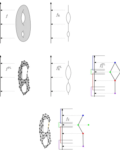
See Figure 2 for an illustration. Note that, since f is constant on equivalence classes, there is an induced map fR : Rf(X) → R such that f = fR◦π, where π is the quotient map X →Rf(X). The topological structure of a Reeb graph can be described if the pair
(X, f) is regular enough. From now on, we will assume that the filter function f :X →R
is Morse-type. Morse-type functions are generalizations of classical Morse functions that share some of their properties without having to be differentiable (nor even defined over a smooth manifold).
Definition 2 Let f be a continuous real-valued function defined on a compact space X. Then f is called of Morse typeif:
(i) There is a finite set Crit(f) = {a1 < ... < an}, called the set of critical values,
such that over every open interval (a0 = −∞, a1), ...,(ai, ai+1), ...,(an, an+1 = +∞)
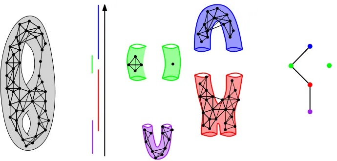
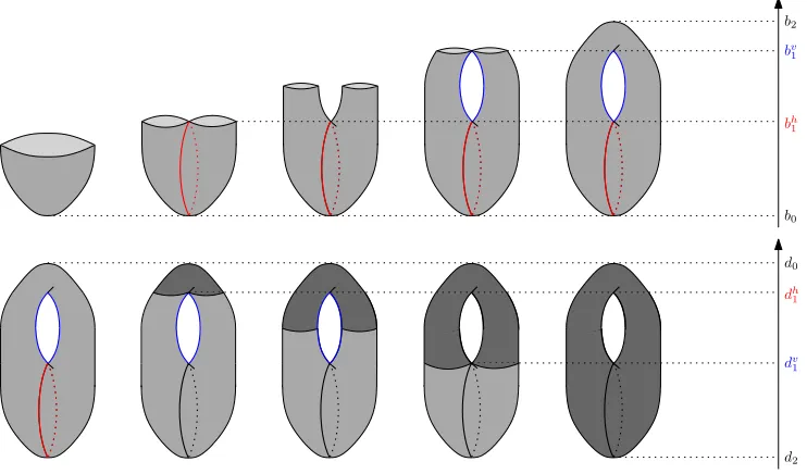
Figure 2: Example of Reeb graph computed on a double torus with the height function. Connected components of the level sets of the function (such as the three different ones drawn on the double torus) are contracted into single points.
(ai, ai+1)→f−1((ai, ai+1)) such that ∀i= 0, ..., n, f|f−1((ai,ai
+1))=π2◦µ −1
i , where π2
is the projection onto the second factor;
(ii) ∀i= 1, ..., n−1, µiextends to a continuous functionµ¯i :Yi×[ai, ai+1]→f−1([ai, ai+1])
and similarly µ0 extends to µ¯0 :Y0×(−∞, a1]→ f−1((−∞, a1]) and µn extends to
¯
µn:Yn×[an,+∞)→f−1([an,+∞));
(iii) Each levelset f−1(t) has a finitely-generated homology.
Key fact 1a. (Proposition 2.10 in de Silva et al. (2016)) For f : X → R a Morse-type function, the Reeb graph Rf(X) is a multigraph.
For our purposes, in the following we further assume that X is a smooth and compact submanifold ofRD. The set of Reeb graphs computed with Morse-type functions over such spaces is denotedRin this article. Whenever it is necessary, it will be equipped with extra structures in the following, such as pseudometrics or topologies.
Mapper. The Mapper is introduced in Singh et al. (2007) as a statistical version of the Reeb graph Rf(X) in the sense that it is a discrete and computable approximation of the
Reeb graph computed with some filter function. Assume that we observe a point cloud Xn = {X1, . . . , Xn} ⊂ X with known pairwise distances. A filter function is chosen and
can be computed on each point ofXn. The generic version of the Mapper algorithm onXn
computed with the filter functionf can be summarized as follows:
1. Cover the range of values Yn =f(Xn) with a set of consecutive intervals {Is}1≤s≤S
which overlap.
2. Apply a clustering algorithm to each pre-image f−1(Is), s ∈ {1, ..., S}. This defines
a pullback cover C={C1,1, . . . ,C1,k1, . . . ,CS,1, . . . ,CS,kS} of the point cloud Xn, where Cs,k denotes thekth cluster of f−1(Is).
3. The Mapper is then the nerve of C. Each vertex vs,k of the Mapper corresponds to
Figure 3: Example of Mapper computed on a sampling of the double torus with the height functionf and a coverI of its range with four open intervals. Clusters are given by a neighborhood graph built on the sampling. Note that the rightmost green vertex is not connected to the other vertices of the Mapper since its corresponding cluster (which contains only one point) has no common points with the others.
See Figure 3 for an illustration. Even for one given filter function, many versions of the Mapper algorithm can be proposed depending on how one chooses the intervals that cover the image of f, and which method is used to cluster the pre-images. Moreover, note that the Mapper can be defined as well for continuous spaces. The definition is strictly the same except for the clustering step, which is replaced by taking the connected components of each pre-imagef−1(Is), s∈ {1, ..., S}.
Our version of Mapper. In this article, we focus on a Mapper algorithm that uses neighborhood graphs. Of course, more sophisticated versions of Mapper can be used in practice but then the statistical analysis is more tricky. We assume that there exists a distance on Xn and that the matrix of pairwise distances is available. First, from the
distance matrix we compute the δ-neighborhood graph built on top of Xn, i.e. we draw
an edge between two different points whenever their pairwise distance is less thanδ. This object plays the role of an approximation of the underlying and unknown metric space X
on which the data are sampled. Second, givenYn=f(Xn) the set of filter values, we choose
a regular cover of Yn with open intervals, where no more than two intervals can intersect
at a time. More precisely, we use open intervals with same length r (apart from the first and the last one, which can have any positive length): ∀s∈ {2, . . . , S−1},
r =`(Is) (1)
where` is the Lebesgue measure onR. The overlap g between two consecutive intervals is also a fixed constant: ∀s∈ {1, . . . , S−1},
0< g= `(Is∩Is+1)
r <
1
The parametersg andr are generally called thegainand theresolutionin the literature on the Mapper algorithm. Finally, for the clustering step, we simply consider the connected components of the pre-imagesf−1(Is) that are induced by the δ-neighborhood graph. The
corresponding Mapper is denoted Mr,g,δ(Xn,Yn) or Mn for short in the following. When
dealing with a continuous spaceX, there is no need to compute a neighborhood graph since the connected components are well-defined, so we let Mr,g(X, f) denote our version of the
Mapper in this case.
Key fact 1b. The Mapper Mr,g,δ(Xn,Yn) is a combinatorial graph.
Moreover, following Carri`ere and Oudot (2017b), we can define a function on the nodes of Mn as follows.
Definition 3 Let v be a node of Mn, i.e. v represents a connected component of f−1(Is)
for some s∈ {1, . . . , S}. Then, we let
fI(v) = mid( ˜Is),
where I˜s =Is\(Is−1∪Is+1) and mid( ˜Is) denotes the midpoint of the interval I˜s.
Filter functions. In practice, it is common to choose filter functions that are coordinate-independent, in order to avoid depending on solid transformations of the data like rotations or translations. The two most common filters that are used in the literature are:
• theeccentricity: x7→supy∈Xd(x, y),
• the eigenfunctions of the covariance matrix as used in Principal Component Analysis.
2.2 Extended persistence signatures and the persistence metric
In this section, we introduce extended persistence and its associated metric, thebottleneck distance, which we will use later to compare Reeb graphs and Mappers. We merely provide a short introduction containing the necessary definitions since the statement of our results does not require a deep understanding of these notions. The understanding of the proofs of these results is more demanding, so we refer the reader willing to read proofs and already familiar with homology to Appendix C for more details, and to Edelsbrunner and Harer (2010); Oudot (2015) for a thorough treatment of extended persistence.
Extended persistence. Given any graphG= (V, E) and a function defined on its nodes f :V →R, the so-calledextended persistence diagramDg(G, f), originally defined in Cohen-Steiner et al. (2009), is a multiset of points in the Euclidean planeR2 that can be computed with extended persistence theory. Each of the diagram points has a specific type, which is either Ord0, Rel1, Ext+0 or Ext
−
Ext+0
Ord0
Rel1
Ext−1
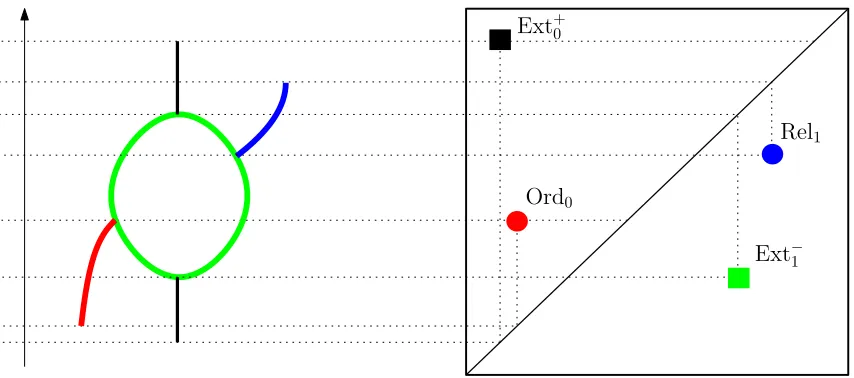
Figure 4: Example of correspondences between topological features of a graph and points in its corresponding extended persistence diagram. Note that ordinary persistence is unable to detect the blue upwards branch.
Topological dictionary. Given a topological space X and a Morse-type function f :
X →R, there is a nice interpretation of Dg(Rf(X), fR) in terms of the structure of Rf(X).
Orienting the Reeb graph vertically sofR is the height function, we can see each connected component of the graph as a trunk with multiple branches (some oriented upwards, others oriented downwards) and holes. Then, one has the following correspondences, where the
vertical span of a feature is the span of its image byfR:
• The vertical spans of the trunks are given by the points in Ext+0(Rf(X), fR);
• The vertical spans of the branches that are oriented downwards are given by the points in Ord0(Rf(X), fR);
• The vertical spans of the branches that are oriented upwards are given by the points in Rel1(Rf(X), fR);
• The vertical spans of the holes are given by the points in Ext−1(Rf(X), fR).
These correspondences provide a dictionary to read off the structure of the Reeb graph from the corresponding extended persistence diagram. See Figure 4 for an illustration.
Note that it is a bag-of-features type descriptor, taking an inventory of all the features (trunks, branches, holes) together with their vertical spans, but leaving aside the actual layout of the features. As a consequence, it is an incomplete descriptor: two Reeb graphs with the same persistence diagram may not be isomorphic.
Definition 4 Given two persistence diagrams D, D0, a partial matchingbetweenDandD0
is a subset Γ of D×D0 such that:
∀p∈D, there is at most onep0∈D0 such that(p, p0)∈Γ,
∀p0 ∈D0, there is at most one p∈D such that(p, p0)∈Γ.
Furthermore, Γ must match points of the same type (ordinary, relative, extended) and of the same homological dimension only. Let ∆ be the diagonal ∆ = {(x, x) : x ∈ R}. The cost of Γ is:
cost(Γ) = max
max
p∈D δD(p), pmax0∈D0 δD 0(p0)
,
where
δD(p) =kp−p0k∞ if ∃p0 ∈D0 such that (p, p0)∈Γ, otherwiseδD(p) = inf
q∈∆kp−qk∞,
δD0(p0) =kp−p0k∞ if ∃p∈D such that (p, p0)∈Γ, otherwise δD0(p0) = inf
q∈∆kp 0−
qk∞. Definition 5 Let D, D0 be two persistence diagrams. The bottleneck distance between D
and D0 is:
d∆(D, D0) = inf
Γ cost(Γ),
where Γ ranges over all partial matchings between D and D0.
Note that d∆ is only a pseudometric and not a true metric, because diagrams which only differ at the diagonal will have zero distance.
Definition 6 Let G1 = (V1, E1) and G2 = (V2, E2) be two combinatorial graphs with
real-valued functions f1 : V1 → R and f2 : V2 → R attached to their nodes. The persistence metric d∆ between the pairs (G1, f1) and (G2, f2) is:
d∆(G1, G2) =d∆(Dg(G1, f1),Dg(G2, f2)).
For a Morse-type function f defined onX and for a finite point cloudXn ⊂ X, we can
thus consider Dg(Rf(X)) = Dg(Rf(X), fR) and Dg(Mn) = Dg(Mn, fI), with fI as in Defi-nition 3. In this context the bottleneck distanced∆(Rf(X),Mn) =d∆(Dg(Rf(X)),Dg(Mn))
is well defined and we use this quantity to assess if the Mapper Mn is a good approximation
2.3 An approximation inequality for Mapper
We are now ready to give the key ingredient of this paper to derive a statistical analysis of the Mapper. The ingredient is an upper bound on the bottleneck distance between the Reeb graph of a pair (X, f) and the Mapper computed with the same filter function f and a specific cover I of a sampled point cloud Xn ⊂ X. From now on, it is assumed that the
underlying space X is a smooth and compact submanifold embedded in RD, and that the filter functionf is Morse-type on X.
Regularity of the filter function. Intuitively, approximating a Reeb graph computed with a filter function f that has large variations is more difficult than for a smooth filter function, for some notion of regularity that we now specify. Our result is given in a general setting by considering the modulus of continuity of f. In our framework, f is assumed to be Morse-type and thus uniformly continuous on the compact setX. Following for instance Section 6 in DeVore and Lorentz (1993), we define the exact modulus of continuity off as:
ωf(δ) = sup
kx−x0k≤δ
|f(x)−f(x0)|
for any δ >0, wherek · k denotes the Euclidean norm in RD. Then ωf satisfies :
1. ωf(δ)→ω(0) = 0 whenδ →0 ;
2. ωf is non-negative and non-decreasing onR+ ;
3. ωf is subadditive : ωf(δ1+δ2)≤ωf(δ1) +ωf(δ2) for anyδ1,δ2 >0; 4. ωf is continous onR+.
In this paper we say that a functionωdefined onR+isa modulus of continuity if it satisfies the four properties above and we say that it isa modulus of continuity forf if, in addition, we have
|f(x)−f(x0)| ≤ω(kx−x0k), for any x, x0 ∈ X.
Theorem 7 Assume that X has positive reach rch and convexity radius ρ. Let Xn be a
point cloud of n points, all lying in X. Assume that the filter function f is Morse-type on
X. Let ω be a modulus of continuity for f. Finally, let r, g be Mapper parameters defined as per Equations (1) and (2). If the three following conditions hold:
δ≤ 1
4min{rch, ρ}, (3)
max{|f(X)−f(X0)| : X, X0 ∈Xn and kX−X0k ≤δ}< gr, (4)
4dH(X,Xn)≤δ, (5)
where dH denotes the Hausdorff distance, then the Mapper Mn = Mr,g,δ(Xn,Yn) with
pa-rameters r,g andδ is such that:
d∆(Rf(X),Mn)≤r+ 2ω(δ). (6)
Analysis of the hypotheses. On the one hand, the scale parameter δ of the neigh-borhood graph could not be smaller than the approximation error corresponding to the Hausdorff distance between the sample and the underlying spaceX (Assumption (5)). On the other hand, it must be smaller than the reach and convexity radius to provide a correct estimation of the geometry and topology of X (Assumption (3)). The quantity gr corre-sponds to the minimum scale at which the filter’s codomain is analyzed. This minimum resolution has to be compared with the regularity of the filter at scaleδ (Assumption (4)). Indeed the pre-images of a filter with strong variations will be more difficult to analyze than when the filter does not vary too fast.
Analysis of the upper bound. The upper bound given in (6) makes sense in that the approximation error is controlled by the resolution level in the codomain and by the regularity of the filter. If one uses a filter with strong variations, or if the grid in the codomain has a too rough resolution, then the approximation will be poor. On the other hand, a sufficiently dense sampling is required in order to take rsmall, as prescribed in the assumptions.
Lipschitz filters. A large class of filters used for the Mapper are actually Lipschitz func-tions and of course, in this case, one can take ω(δ) = cδ for some positive constant c. In particular, c = 1 for linear projections (PCA, SVD, Laplacian or coordinate filter for instance). The distance to a measure (DTM) is also a 1-Lipschitz function, see Chazal et al. (2011). On the other hand, the modulus of continuity of filter functions defined from estimators, e.g. density estimators, is less obvious although still well-defined.
Filter approximation. In some situations, the filter function ˆf used to compute the Mapper is only an approximation of the filter function f with which the Reeb graph is computed. In this context, the pair (Xn,fˆ) appears as an approximation of the pair (X, f).
The following result is directly derived from Theorem 7 and Theorem 5.1 in Carri`ere and Oudot (2017b) (that derives stability for Mappers building on the stability theorem of extended persistence diagrams proved by Cohen-Steiner et al. (2009)):
Corollary 9 Let fˆ:X →R be a Morse-type filter function approximatingf. Assume that Assumptions (3) and (5) of Theorem 7 are satisfied, and assume moreover that
max{max{|f(X)−f(X0)|,|fˆ(X)−fˆ(X0)|} : X, X0∈Xn,kX−X0k ≤δ}< gr. (7)
Then, the MapperMˆn= Mr,g,δ(Xn,fˆ(Xn))built on Xn with filter functionfˆand parameters r, g, δ satisfies:
d∆(Rf(X),Mˆn)≤2r+ 2ω(δ) + max
1≤i≤n|f(Xi)−
ˆ f(Xi)|.
3. Statistical Analysis of Mapper
From now on, the set of observationsXnis assumed to be composed ofnindependent points X1, ..., Xnsampled from a probability distributionPinRD(endowed with its Borel algebra). We assume that each pointXi comes with a filter value which is represented by a random
variable Yi. Contrarily to the Xi’s, the filter values Yi’s are not necessarily independent.
filter f is a deterministic function, in the second one, Yi = ˆf(Xi) where ˆf is an estimator
of the filter function f. In the latter case, the Yi’s are obviously dependent. We first
provide the following proposition, whose proof is deferred to Appendix A.4, which states that computing probabilities on the Mapper makes sense:
Proposition 10 For any fixed choice of parameters r, g, δ and for any fixed n ∈ N, the function
Φ :
(RD)n×Rn → R (Xn,Yn) 7→ Mr,g,δ(Xn,Yn)
is measurable, whereRdenotes the set of Reeb graphs computed from Morse-type functions.
3.1 Statistical Model for the Mapper
In this section, we study the convergence of the Mapper for a general generative model and a class of filter functions. We first introduce the generative model and next we present different settings depending on the nature of the filter function.
Generative model. The set of observationsXnis assumed to be composed ofn
indepen-dent points X1, ..., Xn sampled from a probability distributionP inRD. The support ofP is denotedXP and is assumed to be a smooth and compact submanifold ofRD with positive reach and positive convexity radius, as in the setting of Theorem 7. We also assume that 0<diam(XP)≤L. Next, the probability distributionPis assumed to be (a, b)-standard for some constants a >0 and b≥D, that is for any Euclidean ballB(x, t) centered onx∈ X
with radius t:
P(B(x, t))≥min(1, atb).
This assumption is popular in the literature about set estimation (see for instance Cuevas, 2009; Cuevas and Rodr´ıguez-Casal, 2004). It is also widely used in the TDA literature (Chazal et al., 2015b; Fasy et al., 2014; Chazal et al., 2015a). For instance, when b =D, this assumption is satisfied when the distribution is absolutely continuous with respect to the Hausdorff measure onXP. We introduce the set Pa,b=Pa,b,κ,ρ,L which is composed of all the (a, b)-standard probability distributions for which the support XP is a smooth and compact submanifold of RD with reach larger than κ, convexity radius larger than ρ and diameter less than L.
Filter functions in the statistical setting. The filter function f : XP → R for the Reeb graph is assumed as before to be a Morse-type function. Two different settings have to be considered regarding how the filter function is defined. In the first setting, the same filter function is used to define the Reeb graph and the Mapper. The Mapper can be defined by taking the exact values of the filter function at the observation points f(X1), . . . , f(Xn). Note that this does not mean that the functionf is completely known
the following. It corresponds to PCA or Laplacian eigenfunctions, distance functions (such as the DTM), or regression and density estimators.
Risk of the Mapper. We study, in various settings, the problem of inferring a Reeb graph using Mappers and we use the metric d∆ to assess the performance of the Mapper, seen as an estimator of the Reeb graph. Hence, we study the following quantity:
E[d∆(Mn,Rf(XP))],
where Mn is computed with the exact filter f or the inferred filter ˆf, depending on the
context.
3.2 Reeb graph inference with exact filter and known generative model
We first consider the exact filter setting in the simplest situation where the parameters a and b of the generative model are known. In this setting, for a given neighborhood graph parameter δ, gain g and resolution r, the Mapper Mn = Mr,g,δ(Xn,Yn) is computed with
Yn=f(Xn).
Parameter selection. We now tune the triple of parameters (r, g, δ) depending on the parameters aand b. More precisely, we take:
an arbitraryg∈
1 3,
1 2
, δn= 8
2log(n) an
1/b
, rn=
Vn(δn)+
g , (8)
where Vn(δn) = max{|f(X)−f(X0)| : X, X0 ∈Xn,kX−X0k ≤δn}, andVn(δn)+ denotes
a value that is strictly larger but arbitrarily close toVn(δn).
Upper bound. We give below a general upper bound on the risk of Mn with these
parameters, which depends on the regularity of the filter function and on the parameters of the generative model. We show a uniform convergence over a class of possible filter functions. This class of filters necessarily depends on the support of P, so we define the class of filters for each probability measure inPa,b. For anyP∈ Pa,b, we letF(P, ω) denote the set of filter functionsf :XP →Rsuch thatf is Morse-type on XP with ωf ≤ω.
Proposition 11 Letωbe a modulus of continuity forf such thatω(x)/xis a non-increasing function on R+. For n large enough, the Mapper computed with parameters (rn, g, δn) as
per Equation (8) satisfies
sup
P∈Pa,b
E
"
sup
f∈F(P,ω)
d∆(Rf(XP),Mn)
#
≤C ω
2·8b a
log(n) n
1/b
where the constant C only depends on a, b, and on the geometric parameters of the model.
filter function and on the parameter b which roughly represents the intrinsic dimension of the data. For Lipschitz filter functions, the rate is similar to the one for persistence diagram inference in Chazal et al. (2015b), namely it corresponds to the one of support estimation for the Hausdorff metric (see for instance Cuevas and Rodr´ıguez-Casal (2004)) and Genovese et al. (2012a)). In the other cases where the filters only admit a concave modulus of continuity, we see that the “distortion” created by the filter function slows down the convergence of the Mapper to the Reeb graph.
We now give a lower bound that matches with the upper bound of Proposition 11.
Proposition 12 Let ω be a modulus of continuity for f. Then, for any estimator Rˆn of
Rf(XP),, we have
sup
P∈Pa,b
E
"
sup
f∈F(P,ω)
d∆
Rf(XP),Rˆn
#
≥C ω
1 an
1b ,
where the constant C only depends on a, b and on the geometric parameters of the model.
Propositions 11 and 12 together show that, with the choice of parameters given before, Mn is minimax optimal up to a logarithmic factor log(n) inside the modulus of continuity.
Note that the lower bound is also valid whether or not the coefficientsaandband the filter functionf and its modulus of continuity are given.
3.3 Reeb graph inference with exact filter and unknown generative model We still assume that the exact values Yn = f(Xn) of the filter on the point could can be
computed and that at least a modulus of continuity for the filter is known. However, the parameters a and b are not assumed to be known anymore. We adapt a subsampling ap-proach proposed by Fasy et al. (2014). As before, for a given neighborhood graph parameter δ, gaingand resolutionr, the Mapper Mn= Mr,g,δ(Xn,Yn) is computed with Yn=f(Xn).
Parameter selection. We introduce the sequence sn = (lognn)1+β for some fixed value β >0. Let ˆXsnn be an arbitrary subset ofXn that contains sn points. Then, we take:
an arbitrary g∈
1 3,
1 2
, δn=dH( ˆXnsn,Xn), rn=
Vn(δn)+
g , (9)
whereVn+ is defined as in Equation (8).
Upper bound. Using these parameters, we can then derive the following upper bound: Proposition 13 Let ω be a modulus of continuity for f such that x 7→ ω(x)/x is a non-increasing function. Then, using the same notations as in the previous section, the Mapper
Mn computed with parameters (rn, g, δn) as per Equation (9) satisfies
sup
P∈Pa,b
E
"
sup
f∈F(P,ω)
d∆(Rf(XP),Mn)
#
≤C ω
C0log(n)2+β n
1/b ,
Up to logarithmic factors inside the modulus of continuity, we find that this Mapper is still minimax optimal over the classPa,b by Proposition 12.
3.4 Reeb graph inference with inferred filter and unknown generative model One of the nice properties of the Mapper is that it can be easily computed with any filter function, including estimated filter functions such as PCA eigenfunctions, eccentricity func-tions, DTM funcfunc-tions, Laplacian eigenfuncfunc-tions, density estimators, regression estimators, and many other filters directly estimated from the data. In this section, we assume that the
true filterf is unknown but can be estimated from the data using an estimator ˆf. Without loss of generality, we assume that bothf and ˆf are defined onRD. As before, parametersa andbare not assumed to be known and we have to tune the triple of parameters (rn, g, δn).
Parameter selection. In this context, the quantityVn+ of Equations (8) and (9) cannot be computed as before because there is no direct access to the values off: we only know an estimation ˆf of it. However, in many cases, a modulus of continuityω1 forf is known, which makes possible the tuning of the parameters. For instance, PCA (and kernel) projectors, eccentricity functions, DTM functions (see Chazal et al. (2011)) are all 1-Lipschitz functions, and Corollary 14 below can be applied.
Let ˆVn(δn) = max{|fˆ(X)−fˆ(X0)| : X, X0 ∈ Xn,kX −X0k ≤ δn}, and let ω1 be a modulus of continuity for f. Then, we take:
an arbitraryg∈
1 3,
1 2
, δn=dH( ˆXnsn,Xn), rn=
max{ω1(δn),Vˆn(δn)}+
g . (10)
Upper bound. Following the lines of the proof of Proposition 13 and applying Corol-lary 9, we obtain:
Corollary 14 Let f : RD → R be a Morse-type filter function and let fˆ: RD → R be a
Morse-type estimator of f. Let ω1 (resp. ω2) be a modulus of continuity for f (resp. fˆ).
Let ω = max{ω1, ω2} such that x 7→ ω(x)/x is a non-increasing function. Let also Mˆn =
Mrn,g,δn(Xn,fˆ(Xn)) be the Mapper built on Xn with function fˆand parameters g, δn, rn as
in Equation (10). Then, Mˆn satisfies
E
h d∆
Rf(XP),Mˆn
i
≤Cω
C0log(n)2+β n
1b +E
max
1≤i≤n|f(Xi)−
ˆ f(Xi)|
,
where the constants C, C0 only depends on a, b, and on the geometric parameters of the model.
Note that ω1 has to be known to compute ˆMn in Corollary 14 since it appears in the
definition ofrn. On the contrary,ω2—and thusω—is not required to tune the parameters. PCA eigenfunctions. In the setting of this article, the measureµhas a finite second mo-ment. Following Biau and Mas (2012), we define the covariance operator Γ(·) =E(hX,·iX) and we let Πk denote the orthogonal projection onto the space spanned by the k-th
eigen-vector of Γ. In practice, we consider the empirical version of the covariance operator
ˆ Γn(·) =
1 n
n X
i=1
and the empirical projection ˆΠk onto the space spanned by the k-th eigenvector of ˆΓn.
According to Biau and Mas (2012)(see also Blanchard et al. (2007); Shawe-Taylor et al. (2005)), we have
E
h
kΠk−Πˆkk∞
i =O
1
√
n
.
This, together with Corollary 14 and the fact that both Πk and ˆΠk are 1-Lipschitz, gives
that the rate of convergence of the Mapper of ˆΠk(Xn) computed with parameters δn,g and rn as in Equation (10) (which gives rn=g−1δn+) satisfies
E
h d∆
RΠk(XP),Mrn,g,δn(Xn,Πˆk(Xn)) i
=O max
(
log(n)2+β n
1b ,√1
n )!
.
Hence, the rate of convergence of Mapper is not deteriorated by using ˆΠk instead of Πk if
the intrinsic dimension bof the support ofµ is at least 2.
The distance to measure. It is well known that TDA methods may fail completely in the presence of outliers. To address this issue, Chazal et al. (2011) introduced an alterna-tive distance function which is robust to noise, the distance-to-measure (DTM). A similar analysis as with the PCA filter can be carried out with the DTM filter using the rates of convergence proven in Chazal et al. (2016b).
4. Confidence sets for Reeb signatures
4.1 Confidence sets for extended persistence diagrams
In practice, computing a Mapper Mnand its signature Dg(Mn, fI) is not sufficient: we need to know how accurate these estimations are. One natural way to answer this problem is to provide a confidence set for the Mapper using the bottleneck distance. For α ∈(0,1), we look for some value ηn,α such that
P(d∆(Mn,Rf(XP))≥ηn,α)≤α
or at least such that
lim sup
n→∞ P(d∆(Mn,Rf(
XP))≥ηn,α)≤α.
Let
Mα={R∈ R : d∆(Mn,R)≤α}
be the closed ball of radiusα in the bottleneck distance and centered at the Mapper Mnin
the space of Reeb graphs R. Following Fasy et al. (2014), we can visualize the signatures of the points belonging to this ball in various ways. One first option is to center a box of side length 2α at each point of the extended persistence diagram of Mn—see the right
Several methods have been proposed in Fasy et al. (2014) and Chazal et al. (2014) to define confidence sets for persistence diagrams. We now adapt these ideas to provide confidence sets for Mappers. Except for the bottleneck bootstrap (see Section 4.3), all the methods proposed in these two articles rely on the stability results for persistence diagrams, which say that persistence diagrams equipped with the bottleneck distance are stable under Hausdorff or Wasserstein perturbations of the data. Confidence sets for diagrams are then directly derived from confidence sets in the sample space. Here, we follow a similar strategy using Theorem 7, as explained in the next section.
4.2 Confidence sets derived from Theorem 7
In this section, we always assume that an upper boundωon the exact modulus of continuity ωf of the filter function is known. We start with the following remark: if we can takeδ of
the order ofdH(XP,Xn) in Theorem 7 and if all the conditions of the theorem are satisfied,
thend∆(Mn,Rf(XP)) can be bounded in terms ofω(dH(XP,Xn)). This means that we can
adapt the methods of Fasy et al. (2014) to Mappers.
Known generative model. Let us first consider the simplest situation where the param-etersaanbare also known. Following Section 3.2, we choose forg, δn, rnas per Equation (8).
Let εn =dH(XP,Xn). As shown in the proof of Proposition 11 (see Appendix A.5), for n
large enough, Assumption (3) and (4) are always satisfied and then
P(d∆(Mn,Rf(XP))≥η)≤P
δn≥ω−1
η g−1+ 2
.
Consequently,
P(d∆(Mn,Rf(XP))≥η)≤P(d∆(Mn,Rf(XP))≥η∩εn≤4δn) +P(εn>4δn)
≤Iω(δn)≥ g
1+2gη+ min
1, 2 b
2log(n)n
= Φn(η).
where Φn depends on the parameters of the model (or some bounds on these parameters)
which are here assumed to be known. Hence, given a probability levelα, one has:
P d∆(Mn,Rf(XP))≥Φ
−1
n (α)
≤α.
Unknown generative model. We now assume that a and b are unknown. To com-pute confidence sets for the Mapper in this context, we approximate the distribution of dH(XP,Xn) using the distribution of dH( ˆXsnn ,Xn) conditionally toXn. There areN1= snn
subsets of size sn inside Xn, so we let X1sn, . . . ,XNsn1 denote all the possible configurations.
Define
Ln(t) =
1 N1
N1
X
k=1 IdH(Xk
sn,Xn)>t.
Letsbe the function onN defined bys(n) =sn and lets2n=s(s(n)).There areN2= sn2
n
subsets of size s2n inside Xn. Again, we let Xks2
and we also introduce
Fn(t) =
1 N2
N2
X
k=1 I
dH
Xks2
n ,Xsn
>t.
Proposition 15 Let η >0. Then, one has the following confidence set:
P(d∆(Rf(XP),Mn)≥η)≤Fn
1 4ω
−1
g 1 + 2gη
+Ln
1 4ω
−1
g 1 + 2gη
+osn n
14 .
Both Fn and Ln can be computed in practice, or at least approximated using Monte
Carlo procedures. The upper bound on P(d∆(Rf(XP),Mn)≥η) then provides an
asymp-totic confidence region for the persistence diagram of the Mapper Mn, which can be
explic-itly computed in practice. See the green squares in the first row of Figure 5. The main drawback of this approach is that it requires knowing a modulus of continuityω and, more importantly, the number of observations has to be very large, which is not the case on our examples in Section 5.
Modulus of continuity of the filter function. As shown in Proposition 15, the mod-ulus of continuity of the filter function is a key quantity to describe the confidence regions. Inferring the modulus of continuity of the filter from the data is a tricky problem. For-tunately, in practice, even in the inferred filter setting, a modulus of continuity for the function is known in many situations. For instance, projections such as PCA eigenfunctions and DTM functions are 1-Lipschitz.
4.3 Bottleneck Bootstrap
The two methods given before both require an explicit upper bound on the modulus of continuity of the filter function. Moreover, these methods both rely on the approximation result Theorem 7, which often leads to conservative confidence sets. An alternative strategy is the bottleneck bootstrap introduced in Chazal et al. (2014), and which we now apply to our framework.
Bootstrap. The bootstrap is a general method for estimating standard errors and com-puting confidence intervals. Let Pn be the empirical measure defined from the sample
(X1, Y1), . . . ,(Xn, Yn). Let (X1∗, Y1∗). . . ,(Xn∗, Yn∗) be a sample from Pn and let also M∗n be
the random Mapper defined from this sample. We then take for ˆηn,α the quantity ˆη∗n,α
defined by
P d∆(M∗n,Mn)>ηˆ∗n,α|X1, . . . , Xn
=α. (11)
Note that ˆηn,α∗ can be easily estimated with Monte Carlo procedures. It has been shown in Chazal et al. (2014) that the bottleneck bootstrap is valid when computing the sublevel sets of a density estimator. The validity of the bottleneck bootstrap has not been proven for the extended persistence diagram of any distance function. For Mapper, it would require writingd∆(M∗n,Mn) in terms of the distance between the extrema of the filter function and
Extension of the analysis. As pointed out in Section 2.1, many versions of the Mapper exist in the literature. One of them, called theedge-based MultiNerve MapperM4r,g,δ(Xn,Yn),
is described in Section 8 of Carri`ere and Oudot (2017b). The main advantage of this ver-sion is that it allows for finer resolutions than the usual Mapper while remaining fast to compute. Our analysis can actually handle this version as well by replacing gr by r in Assumption (4) of Theorem 7—see Remark 8, and changing constants accordingly in the proofs. In particular, this improves the resolutionrn in Equation (9) sinceg−1Vn(δn)+
be-comesVn(δn)+. Hence, we use this edge-based version in Section 5, where this improvement
on the resolutionrn allows us to compensate for the low number of observations.
5. Numerical experiments
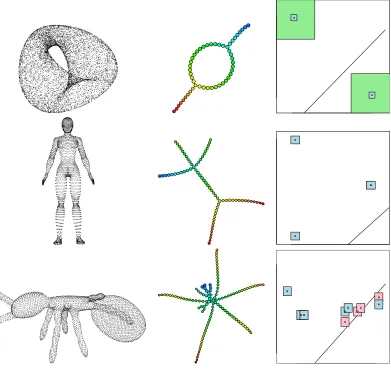
In this section, we provide few examples of parameter selections and confidence regions (which are unions of squares in the extended persistence diagrams) obtained with bot-tleneck bootstrap. The interpretation of these regions is that squares that intersect the diagonal, which are drawn in pink color, represent topological features in the Mappers that may be horizontal or artifacts due to the cover, and that may not be present in the Reeb graph. We show in Figure 5 various Mappers (in each node of the Mappers, the left num-ber is the cluster ID and the right numnum-ber is the numnum-ber of observations in that cluster) and 85 percent confidence regions computed on various data sets. All δ parameters and resolutions were computed with Equation (9) (the δ parameters were also averaged over N = 100 subsamplings with β = 0.001), and all gains were set to 40%. The code we used is available in the Gudhi open source library (see Carri`ere (2017)). The confidence regions were computed by bootstrapping data 100 times. Note that computing confidence regions with Proposition 15 is possible, but the numbers of observations in all of our data sets were too low, leading to conservative confidence regions that did not allow for interpretation.
5.1 Mappers and confidence regions
Synthetic example. We computed the Mapper of an embedding of the Klein bottle into R4 with 10,000 points with the height function. In order to illustrate the conserva-tivity of confidence regions computed with Proposition 15, we also plot these regions for an embedding with 10,000,000 points using the fact that the height function is 1-Lipschitz. Corresponding squares are drawn in green color. Their very large sizes show that Propo-sition 15 requires a very large number of observations in practice. See the first row of Figure 5.
3D shapes. We computed the Mapper of an ant shape and a human shape from Chen et al. (2009) embedded inR3 (with 4,706 and 6,370 points respectively) Both Mappers were computed with the height function. One can see that the confidence squares for the features that are almost horizontal (such as the small branches in the Mapper of the ant) intersect indeed the diagonal. See the second and third rows of Figure 5.
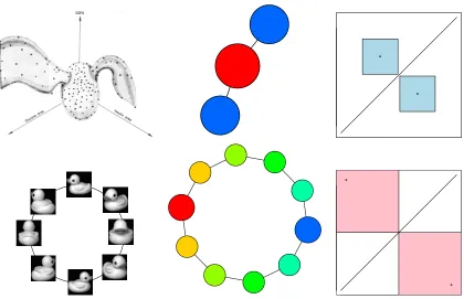
Figure 6: Mappers computed with automatic tuning (middle) and 85 percent confidence regions for their topological features (right) are provided for the Reaven-Miller data set (first row) and the COIL data set (second row).
the projection pursuit method, and in Singh et al. (2007), the authors applied Mapper with hand-crafted parameters to get back this result. Here, we normalized the data to zero mean and unit variance, and we obtained the two flares in the Mapper computed with the eccentricity function. Moreover, these flares are at least 85 percent sure since the confidence squares on the corresponding points in the extended persistence diagrams do not intersect the diagonal. See the first row of Figure 6.
COIL data set. The second data set is an instance of the 16,384-dimensional COIL data set of Nene et al. (1996). It contains 72 observations, each of which being a picture of a duck taken at a specific angle. Despite the low number of observations and the large number of dimensions, we managed to retrieve the intrinsic loop lying in the data using the first PCA eigenfunction. However, the low number of observations made the bootstrap fail since the confidence squares computed around the points that represent this loop in the extended persistence diagram intersect the diagonal. See the second row of Figure 6.
5.2 Noisy data
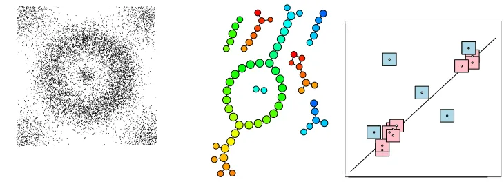
Figure 7: Mappers computed with automatic tuning (middle) and 85 percent confidence regions for their topological features (right) are provided for a noisy crater in the Euclidean plane.
use an alternative filtration of simplicial complexes instead of the Rips filtration. A first option is to consider the upper level sets of a density estimator rather than the distance to the sample (see Section 4.4 in Fasy et al. (2014)). Another solution is to consider the sublevel sets of the DTM and apply persistence homology inference in Chazal et al. (2014).
Crater data set. To handle noise in our crater data set, we simply smoothed the data set by computing the empirical DTM with 10 neighbors on each point and removing all points with DTM less than 40 percent of the maximum DTM in the data set. Then we computed the Mapper with the height function. One can see that all topological features in the Mapper that are most likely artifacts due to noise (like the small loops and con-nected components) have corresponding confidence squares that intersect the diagonal in the extended persistence diagram. See Figure 7.
6. Conclusion
In this article, we provided a statistical analysis of the Mapper. Namely, we proved the fact that the Mapper is a measurable construction in Proposition 10, and we used the ap-proximation Theorem 7 to show that the Mapper is a minimax optimal estimator of the Reeb graph in various contexts—see Propositions 11, 12 and 13—and that corresponding confidence regions can be computed—see Proposition 15 and Section 4.3. Along the way, we derived rules of thumb to automatically tune the parameters of the Mapper with Equa-tions (8), (9) and (10). Finally, we provided few examples of our methods on various data sets in Section 5.
Future directions. We plan to investigate several questions for future work.
• We believe that using weighted versions ofδ-neighborhood graphs, as defined in Buchet et al. (2015), would improve the quality of the confidence regions on the Mapper fea-tures, and would probably be a better way to deal with noise that our current solution.
• We plan to adapt our statistical setting to the question of selecting variables, which is one of the main applications of the Mapper in practice.
Acknowledgements. This work was supported by ERC grant Gudhi (ERC-2013-ADG-339025) and by ANR project TopData (ANR-13-BS01-0008). The authors would like to thank the anonymous referees for their constructive criticism and comments. The third author acknowledges the support of ICERM and Brown University, as part of this work was carried out while he was participating in the ICERM program Topology in Motion during the Fall of 2016.
Appendix A. Proofs
A.1 Preliminary results
In order to prove the results of this article, we need to state several preliminary definitions and theorems. All of them can be found, together with their proofs, in Dey and Wang (2013) and Carri`ere and Oudot (2017b). In this section, we letXn⊂ X be a point cloud of npoints sampled on a smooth and compact submanifoldX embedded inRD, with positive reach rch and convexity radius ρ. Since δ-neighborhood graphs can be seen as 1-skeletons of Rips complexes with parameter δ, as per Definition 55 in Carri`ere and Oudot (2017b), and since many results are phrased with Rips complexes in the literature, we also use these complexes to state our results in this section. Letf :X →Rbe a Morse-type filter function,
I be an open cover of the range off with resolution r and gain g < 12 (which ensures that no more than two cover elements can intersect at once, i.e. the cover is minimal), and
|Ripsδ(Xn)| denote a geometric realization of the Rips complex built on top of Xn with
parameter δ, and fPL :|Ripsδ(Xn)| →R be the piecewise-linear interpolation of f on the simplices of Ripsδ(Xn).
Definition 16 Let G= (Xn, E) be a graph built on top of Xn. Let e= (X, X0)∈E be an
edge of G, and let I(e) be the open interval (min{f(X), f(X0)},max{f(X), f(X0)}). Then
e is said to be intersection-crossing if there is a pair of consecutive intervals I, J ∈ I such that∅ 6=I ∩J ⊆I(e).
Theorem 17 (Lemma 61 and 62 in Carri`ere and Oudot (2017b)). Let Rips1δ(Xn)
de-note the 1-skeleton of Ripsδ(Xn). If Rips1δ(Xn) has no intersection-crossing edges, then
Mr,g,δ(Xn, f(Xn)) andMr,g(|Ripsδ(Xn)|, fPL) are isomorphic as combinatorial graphs.
Theorem 18 (Theorem 54 in Carri`ere and Oudot (2017b)). Letf :X →Rbe a Morse-type
function. Then, we have the following inequality between extended persistence diagrams:
d∆(Dg(Rf(X), fR),Dg(Mr,g(X, f), fI))≤r. (12)
Moreover, given another Morse-type function fˆ:X →R, we have:
Theorem 19 (Theorem 4.6, Remark 2 in Dey and Wang (2013) and Theorem 59 in Carri`ere and Oudot (2017b)). If 4dH(X,Xn)≤δ≤min{rch/4, ρ/4}, then:
d∆(Dg(Rf(X), fR),Dg(RfPL(|Ripsδ(Xn)|), fRPL))≤2ω(δ).
Note that the original version of this theorem is only proven for Lipschitz functions in Dey and Wang (2013), but it extends at no cost to functions with modulus of continuity.
A.2 Proof of Theorem 7
Let |Ripsδ(Xn)| denote a geometric realization of the Rips complex built on top of Xn
with parameter δ. Moreover, let fPL :|Ripsδ(Xn)| →R be the piecewise-linear interpola-tion of f on the simplices of Ripsδ(Xn), whose 1-skeleton is denoted by Rips1δ(Xn). Since
(|Ripsδ(Xn)|, fPL) is a metric space, we also consider its Reeb graph RfPL(|Ripsδ(Xn)|),
with induced function fPL
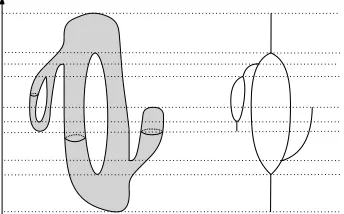
R , and its Mapper Mr,g(|Ripsδ(Xn)|, fPL), with induced function fIPL. See Figure 8. Then, the following inequalities lead to the result:
d∆(Rf(X),Mn) =d∆(Dg(Rf(X), fR),Dg(Mn, fI)) =d∆ Dg(Rf(X), fR),Dg(Mr,g(|Ripsδ(Xn)|, fPL), fIPL)
(14)
≤d∆ Dg(Rf(X), fR),Dg(RfPL(|Ripsδ(Xn)|), fRPL)
+d∆ Dg(RfPL(|Ripsδ(Xn)|), fRPL),Dg(Mr,g(|Ripsδ(Xn)|, fPL), fIPL)
(15)
≤2ω(δ) +r. (16)
Let us prove every (in)equality:
Equality (14). Let X1, X2 ∈Xn such that (X1, X2) is an edge of Rips1δ(Xn) i.e. kX1−
X2k ≤δ. Then, according to (4): |f(X1)−f(X2)|< gr. Hence, there is nos∈ {1, . . . , S−1} such thatIs∩Is+1⊆[min{f(X1), f(X2)},max{f(X1), f(X2)}]. It follows that there are no intersection-crossing edges in Rips1δ(Xn). Then, according to Theorem 17, there is a graph
isomorphism i : Mn = Mr,g,δ(Xn, f(Yn)) → Mr,g(|Ripsδ(Xn)|, fPL). SincefI =fIPL◦i by definition offI and fIPL, the equality follows.
Inequality (15). This inequality is just an application of the triangle inequality. Inequality (16). According to (3), we have δ≤min{rch/4, ρ/4}. According to (5), we also have δ≥4dH(X,Xn). Hence, we have
d∆(Dg(Rf(X), fR),Dg(RfPL(|Ripsδ(Xn)|), fRPL))≤2ω(δ),
according to Theorem 19. Moreover, we have
d∆(Dg(RfPL(|Ripsδ(Xn)|), fRPL),Dg(Mr,g(|Ripsδ(Xn)|, fPL), fIPL))≤r,
f
f
Rf
PLf
RPLf
IPLf
IA.3 Proof of Corollary 9
Let|Ripsδ(Xn)|denote a geometric realization of the Rips complex built on top of Xnwith
parameterδ. Moreover, letfPL:|Ripsδ(Xn)| →Rbe the piecewise-linear interpolation off on the simplices of Ripsδ(Xn), whose 1-skeleton is denoted by Rips1δ(Xn). Similarly, let ˆfPL
be the piecewise-linear interpolation of ˆf on the simplices of Rips1δ(Xn). As before, since
(|Ripsδ(Xn)|, fPL) and (|Ripsδ(Xn)|,fˆPL) are metric spaces, we also consider their Mappers
Mr,g(|Ripsδ(Xn)|, fPL) and Mr,g(|Ripsδ(Xn)|,fˆPL). Then, the following inequalities lead to
the result:
d∆(Rf(X),Mˆn)≤d∆(Rf(X),Mn) +d∆(Mn,Mˆn) by the triangle inequality
=d∆(Rf(X),Mn) +d∆(Mr,g(|Ripsδ(Xn)|, fPL),Mr,g(|Ripsδ(Xn)|,fˆPL)) (17)
≤r+ 2ω(δ) +d∆(Mr,g(|Ripsδ(Xn)|, fPL),Mr,g(|Ripsδ(Xn)|,fˆPL)) by Theorem 7
≤r+ 2ω(δ) +r+kfPL−fˆPLk∞ by Equation (13) = 2r+ 2ω(δ) + max{|f(X)−fˆ(X)| : X ∈Xn}
Let us prove Equality (17). By definition of r, there are no intersection-crossing edges for bothf and ˆf. According to Theorem 17, Mr,g(|Ripsδ(Xn)|, fPL) and Mnare isomorphic
and similarly for Mr,g(|Ripsδ(Xn)|,fˆPL) and ˆMn. See also the proof of Equality (14).
A.4 Proof of Proposition 10
We check that not only the topological signature of the Mapper but also the Mapper itself is a measurable object and thus can be seen as an estimator of a target Reeb graph. This problem is more complicated than for the statistical framework of persistence diagram inference, for which the existing stability results give for free that persistence estimators are measurable for adequate sigma algebras.
Let ¯R=R∪ {+∞}denote the extended real line. Given a fixed integer n≥1, let C[n] be the set of abstract simplicial complexes over a fixed set of n vertices. We see C[n] as a subset of the power set 22[n], where [n] ={1,· · ·, n}, and we implicitly identify 2[n]with the set [2n] via the map assigning to each subset {i1,· · ·, ik}the integer 1 +Pkj=12ij−1. Given a fixed parameterδ >0, we define the application
Φ1:
(
(RD)n×Rn → C[n]×R¯2 [n]
(Xn,Yn) 7→ (K, fK)
whereK is the abstract Rips complex of parameterδover thenlabeled points inRD, minus the intersection-crossing edges and their cofaces, and where fK is a function defined by:
fK :
2[n] → R¯
σ 7→
(
maxi∈σYi ifσ ∈K
The space (RD)n×Rnis equipped with the standard topology, denoted byT1, inherited fromR(D+1)n. The spaceC[n]×R¯2
[n]
is equipped with the product, denoted byT2 hereafter, of the discrete topology onC[n]and the topology induced by the extended distanced(f, g) = max{|f(σ)−g(σ)| : σ ∈ 2[n], f(σ) or g(σ) 6= +∞} on ¯R2
[n]
. In particular, K 6= K0 ⇒
d(fK, fK0) = +∞.
Note that the map (Xn,Yn) 7→ K is piecewise-constant, with jumps located at the
hypersurfaces defined by kXi−Xjk2 =δ2 (for combinatorial changes in the Rips complex)
orYi = cst∈End((r, g)) (for changes in the set of intersection-crossing edges) in (RD)n×Rn, where End((r, g)) denotes the set of endpoints of elements of the gomic (r, g). We can then define a finite measurable partition (C`)`∈L of (RD)n×Rn whose boundaries are included in these hypersurfaces, and such that (Xn,Yn) 7→ K is constant over each set C`. As a
byproduct, we have that (Xn,Yn)7→f is continuous over each setC`.
We now define the operator
Φ2 :
(
C[n]×R¯2[n]
→ A
(K, f) 7→ (|K|, fPL)
whereAdenotes the class of topological spaces filtered by Morse-type functions, and where fPL is the piecewise-linear interpolation of f on the geometric realization |K| of K. For a fixed simplicial complex K, the extended persistence diagram of the lower-star filtration induced byf and of the sublevel sets offPLare identical—see e.g. Morozov (2008), therefore the map Φ2is distance-preserving (hence continuous) in the pseudometricsd∆on the domain and codomain. Since the topologyT2 onC[n]×R¯2
n
is a refinement2 of the topology induced by d∆, the map Φ2 is also continuous when C[n]×R¯2
[n]
is equipped with T2.
Let now Φ3 :A → Rmap each Morse-type pair (X, f) to its Mapper Mf(X,I), where
I = (r, g) is the gomic induced by r and g. Note that, similarly to Φ1, the map Φ3 is piecewise-constant, since combinatorial changes in Mf(X,I) are located at the regions
Crit(f)∩End(I) 6=∅. Hence, Φ3 is measurable in the pseudometricd∆. For more details on Φ3, we refer the reader to Definition 7.6 in Carri`ere and Oudot (2017b).
Moreover, MfPL(|K|,I) is isomorphic to Mr,g,δ(Xn,Yn) by Theorem 17 since all of the
intersection-crossing edges were removed in the construction of K. Hence, the map Φ defined by Φ = Φ3◦Φ2◦Φ1 is a measurable map that sends (Xn,Yn) to Mr,g,δ(Xn,Yn).
A.5 Proof of Proposition 11
We fix some parametersa >0 andb≥1. First note that Assumption (4) is always satisfied by definition of rn. Next, there existsn0 ∈N such that for anyn≥n0, Assumption (3) is satisfied because δn→0 and ω(δn)→0 as n→+∞. Moreover, n0 can be taken the same for all f ∈S
P∈P(a,b)F(P, ω).
Let εn = dH(X,Xn). Under the (a, b)-standard assumption, it is well known that (see
for instance Cuevas and Rodr´ıguez-Casal (2004); Chazal et al. (2015b)):
P(εn≥u)≤min
1, 4 b
aube
−a(u
2)
b n
,∀u >0. (18)
In particular, regarding the complementary of (5) we have:
P
εn>
δn
4
≤min
1, 2 b
2log(n)n
. (19)
Recall that diam(XP) ≤ L. Let ¯C = ω(L) be a constant that only depends on the parameters of the model. Then, for any P∈ P(a, b), we have:
sup
f∈F(P,ω)
d∆(Rf(XP),Mn)≤C.¯ (20)
Forn≥n0, we have : sup
f∈F(P,ω)
d∆(Rf(XP),Mn) = sup f∈F(P,ω)
d∆(Rf(XP),Mn) Iεn>δn/4
+ sup
f∈F(P,ω)
d∆(Rf(XP),Mn) Iεn≤δn/4
and thus
E
"
sup
f∈F(P,ω)
d∆(Rf(XP),Mn) #
≤ C¯P
εn>
δn
4
+rn+ 2ω(δn)
≤ C¯min
1, 2 b
2log(n)n
+
1 + 2g g
ω(δn) (21)
where we have used (20), Theorem 7 and the fact thatVn(δn)+ can be chosen less or equal
toω(δn). Fornlarge enough, the first term in (21) is of the order ofδnb, which can be upper
bounded by δn and thus byω(δn) (up to a constant) sinceω(δ)/δ is non-increasing. Since
1+2g
g <6 because
1
3 < g < 1
2, we get that the risk is bounded by ω(δn) for n≥ n0 up to a constant that only depends on the parameters of the model. The same inequality is of course valid for any n by taking a larger constant, because n0 itself only depends on the parameters of the model.
A.6 Proof of Proposition 12
The proof follows closely Section B.2 in Chazal et al. (2015b). Let X0 = [0, a−1/b] ⊂RD.
Obviously, X0 is a smooth and compact submanifold of RD. Let U(X0) be the uniform measure on X0. Let Pa,b,X0 denote the set of (a, b)-standard measures whose support is
included inX0. Let x0 = 0∈ X0 and{xn}n∈N∗ ∈ X0N such thatkxn−x0k= (an)−1/b. Now, let
f0 :
X0 →R
x 7→ω(kx−x0k)
Rf0|X
P
(XP). Then, we have:
sup
P∈Pa,b
E
"
sup
f∈F(P,ω)
d∆
Rf(XP),Rˆn
#
≥ sup
P∈Pa,b,X0 E
"
sup
f∈F(P,ω)
d∆
Rf(XP),Rˆn
#
≥ sup
P∈Pa,b,X0 E
h d∆
Rf0|X
P(
XP),Rˆn i
= sup
P∈Pa,b,X0 E
h ρ
θ0(P),Rˆn i
,
where ρ = d∆. For any n ∈ N∗, we let P0,n = δx0 be the Dirac measure on x0 and P1,n = (1−1n)P0,n+1nU([x0, xn]). As a Dirac measure, P0,n is obviously inPa,b,X0. We now
check that P1,n∈ Pa,b,X0.
• Let us studyP1,n(B(x0, r)). Assume r≤(an)−1/b. Then
P1,n(B(x0, r)) = 1− 1 n+
1 n
r (an)−1/b ≥
1− 1
n+ 1 n
r (an)−1/b
b ≥ 1 2+ 1 n
anrb ≥arb.
Assume r >(an)−1/b. Then
P1,n(B(x0, r)) = 1≥min{arb}. • Let us studyP1,n(B(xn, r)). Assumer≤(an)−1/b. Then
P1,n(B(xn, r)) =
1 n
r (an)−1/b ≥
1 n
r (an)−1/b
b
=arb.
Assume r >(an)−1/b. Then
P1,n(B(xn, r)) = 1≥min{arb}.
• Let us studyP1,n(B(x, r)), wherex∈(x0, xn). Assume r ≤x. Then
P1,n(B(x, r))≥
1 n
r
(ab)−1/b ≥ar
b (see previous case).
Assume r > x. ThenP1,n(B(x, r)) = 1−n1 +1n(
x+min{r,(an)−1/b−x})
(an)−1/b .
If min{r, (an)−1/b−x}=r, then we have
P1,n(B(x, r))≥1−
1 n+
1 n
r
(ab)−1/b ≥ar
b (see previous case).
Otherwise, we have
ThusP1,n is inPa,b,X0 as well. Hence, we apply Le Cam’s lemma (see Section B) to get:
sup
P∈Pa,b,X0 E
h ρ
θ0(P),Rˆn i
≥ 1
8ρ(θ0(P0,n), θ0(P1,n)) [1−TV(P0,n,P1,n)] 2n
.
By definition, we have:
ρ(θ0(P0,n), θ0(P1,n)) =d∆
Rf0|{x0}({x0}),Rf0|[x0,xn](U[x0, xn])
.
Since DgRf0|{x0}({x0})
={(0,0)} and DgRf0|[x0,xn](U[x0, xn])
={(f(x0), f(xn))}
be-cause f0 is increasing by definition ofω, it follows that
ρ(θ0(P0,n), θ0(P1,n)) =
1
2|f(xn)−f(x0)|= 1 2ω
(an)−1/b. It remains to compute TV(P0,n,P1,n) =
1− 1− 1 n
+1
n(an)
−1/b= 1
n+o
1
n
. The propo-sition follows then from the fact that [1−TV(P0,n,P1,n)]2n→e−2.
A.7 Proof of Proposition 13
Let P ∈ Pa,b and ω a modulus of continuity for f. Using the same notation as in the
previous section, we have
P(δn≥u)≤P
dH(Xn,XP)≥
u 2
+P
dH(Xsnn ,XP)≥
u 2
≤P
εn≥
u 2
+P
εsn ≥
u 2
. (22)
Note that for any f ∈ F(P, ω), according to (6) and (20)
d∆(Rf(XP),Mn)≤[r+ 2ω(δ)]IΩn+ ¯CIΩcn (23)
where Ωn is the event defined by
Ωn={4δn≤min{κ, ρ}} ∩ {4εn≤δn}.
This gives
E
"
sup
f∈F(P,ω)
d∆(Mn,Rf(X)) #
≤
Z C¯
0 P
ω(δn)≥ g 1 + 2gα
dα
| {z }
(A)
+ ¯CP
εn≥
δn
4
| {z }
(B) + ¯CP
δn≥min nκ
4, ρ 4
o
| {z }
(D)
.
Let us bound the three terms (A), (B) and (C).
• Term(B). Lettn= 2
2log(n) an
1/b
andAn={εn< tn}. We first prove thatδn≥4εn
on the eventAn, fornlarge enough. We follow the lines of the proof of Theorem 3 in
Section 6 in Fasy et al. (2014).
Let qn be the tn-packing numberof XP, i.e. the maximal number of Euclidean balls
B(X, tn)∩XP, whereX∈ XP, that can be packed intoXPwithout overlap. It is known
(see for instance Lemma 17 in Fasy et al. (2014)) that qn = Θ(t−nd), where d is the
(intrinsic) dimension of XP. Let Packn = {c1,· · ·, cqn} be a corresponding packing
set, i.e. the set of centers of a family of balls of radius tn whose cardinality achieves
the packing number qn. Note that dH(Packn,XP) ≤ 2tn. Indeed, for any X ∈ XP,
there must exist c ∈ Packn such that kX −ck ≤ 2tn, otherwise X could be added
to Packn, contradicting the fact that Packn is maximal. By contradiction, assume n< tn andδn≤4n. Then:
dH(Xsnn ,Packn)≤dH(Xsnn ,Xn) +dH(Xn,XP) +dH(XP,Packn)
≤5dH(Xn,XP) + 2tn≤7tn.
Now, one has qnsn = Θlog(nn1)−1−b/db/d+β
. Since b ≥D ≥d by definition, it follows that sn= o(qn). In particular, this means that dH(Xsnn ,Packn) >7tn forn large enough,
which yields a contradiction.
Hence, one hasδn≥4εn on the eventAn. Thus, one has:
P
εn≥
δn
4
≤P
εn≥
δn
4 |An
| {z }
=0
P(An) +P(Anc) =P(Acn).
Finally, the probability ofAcnis bounded with (18):
P(Acn)≤
2b 2log(n)n.
• Term (A). This is the dominating term. First, note that since ω is increasing, one has for allu >0:
P(ω(δn)≥u) =P δn≥ω−1(u)
. (24)
Then, using (22) and (24), we have:
(A)≤
Z C¯
0 P
εn≥
1 2ω
−1
gα 1 + 2g
dα+
Z C¯
0 P
εsn ≥
1 2ω
−1
gα 1 + 2g
dα.
We only bound the first integral, but the analysis extends verbatim to the second integral when replacingn bysn. Let
αn=
1 + 2g
g ω
"
4blog(n) an
Since x7→ ω(xx) is non-increasing, it follows that x7→ ω−1x(x) is non-decreasing, and ω−1(x)≥ x
yω
−1(y), ∀x≥y >0. (25)
Taking inspiration from Section B.2 in Chazal et al. (2015b) and using (18), we have the following inequalities:
Z C¯
0 P
εn≥
1 2ω
−1
gα 1 + 2g
dα
≤αn+
8b a
Z C¯ αn
1
ω−1 gα
1+2g bexp
"
−an
4bω
−1
gα 1 + 2g
b# dα
≤αn+
8b a
Z C¯ αn
αbn h
αω−1gαn
1+2g
ibexp "
− anα
b
(4αn)b ω−1
gαn
1 + 2g b#
dα
≤αn+αn
2b4n1−1/b ba1/bω−1gαn
1+2g
Z
u≥an
4bω−1
gαn
1+2g bu
1/b−2 e−udu
=αn+αn
2bn blog(n)1/b
Z
u≥log(n)
u1/b−2e−udu≤
1 + 2
b
blog(n)2
αn sinceb≥1
≤C(b)αn,
where we used (25) with x = 1+2gαg and y = 1+2gαng for the second inequality. The constantC(b) only depends on b.
Hence, since 1+2gg < 6, there exist constants K, K0 > 0 that depend only of the geometric parameters of the model such that:
(A)≤Kω
K0log(sn) sn
1/b .
Final bound. Since sn =nlog(n)−(1+β), by gathering all four terms, there exist
con-stants C, C0 >0 such that:
E
"
sup
f∈F(P,ω)
d∆(Rf(XP),Mn)
#
≤Cω
C0log(n)2+β n
1/b .
A.8 Proof of Proposition 15
We have the following bound by using (23) in the proof of Proposition 13:
P(d∆(,Rf(XP),Mn)≥η)
≤P
ω(δn)≥ g 1 + 2gη
+P
εn≥
δn
4
+P
δn≥min nκ 4, ρ 4 o ≤P εn≥
1 2ω
−1
g 1 + 2gη
+P
εsn ≥
1 2ω
−1
g 1 + 2gη
+o
1 nlog(n)