Finding All Bayesian Network Structures within a Factor of Optimal

The Thirty-Third AAAI Conference on Artificial Intelligence (AAAI-19)

Finding All Bayesian Network Structures within a Factor of Optimal

Zhenyu A. Liao,

Charupriya Sharma,

James Cussens,

Peter van Beek

2_{Department of Computer Science, University of York, York, United Kingdom} {z6liao, c9sharma, vanbeek}@uwaterloo.ca, james.cussens@york.ac.uk

Abstract

A Bayesian network is a widely used probabilistic graphical model with applications in knowledge discovery and predic-tion. Learning a Bayesian network (BN) from data can be cast as an optimization problem using the well-known score-and-search approach. However, selecting a single model (i.e., the best scoring BN) can be misleading or may not achieve the best possible accuracy. An alternative to committing to a sin-gle model is to perform some form of Bayesian or frequentist model averaging, where the space of possible BNs is sam-pled or enumerated in some fashion. Unfortunately, existing approaches for model averaging either severely restrict the structure of the Bayesian network or have only been shown to scale to networks with fewer than 30 random variables. In this paper, we propose a novel approach to model averaging inspired by performance guarantees in approximation algo-rithms. Our approach has two primary advantages. First, our approach only considerscrediblemodels in that they are op-timal or near-opop-timal in score. Second, our approach is more efficient and scales to significantly larger Bayesian networks than existing approaches.

Introduction

A Bayesian network is a widely used probabilistic graphical model with applications in knowledge discovery, explana-tion, and prediction (Darwiche 2009, Koller and Friedman 2009). A Bayesian network (BN) can be learned from data using the well-knownscore-and-search approach, where a scoring function is used to evaluate the fit of a proposed BN to the data, and the space of directed acyclic graphs (DAGs) is searched for the best-scoring BN. However, selecting a single model (i.e., the best-scoring BN) may not always be the best choice. When one is using BNs for knowledge dis-covery and explanation with limited data, selecting a single model may be misleading as there may be many other BNs that have scores that are very close to optimal and the pos-terior probability of even the best-scoring BN is often close to zero. As well, when one is using BNs for prediction, se-lecting a single model may not achieve the best possible ac-curacy.

An alternative to committing to a single model is to per-form some per-form of Bayesian or frequentist model averag-ing (Claeskens and Hjort 2008, Hoetaverag-ing et al. 1999, Koller

Copyright c2019, Association for the Advancement of Artificial Intelligence (www.aaai.org). All rights reserved.

and Friedman 2009). In the context of knowledge discovery, Bayesian model averaging allows one to estimate, for exam-ple, the posterior probability that an edge is present, rather than just knowing whether the edge is present in the best-scoring network. Previous work has proposed Bayesian and frequentist model averaging approaches to network struc-ture learning that enumerate the space of all possible DAGs (Koivisto and Sood 2004), sample from the space of all pos-sible DAGs (He, Tian, and Wu 2016, Madigan and Raftery 1994), consider the space of all DAGs consistent with a given ordering of the random variables (Buntine 1991, Dash and Cooper 2004), consider the space of tree-structured or other restricted DAGs (Madigan and Raftery 1994, Meil˘a and Jaakkola 2000), and consider only the k-best scoring DAGs for some given value of k (Chen, Choi, and wiche 2015, Chen, Choi, and Darwiche 2016, Chen, Dar-wiche, and Choi 2018, Chen and Tian 2014, He, Tian, and Wu 2016, Tian, He, and Ram 2010). Unfortunately, these existing approaches either severely restrict the structure of the Bayesian network, such as only allowing tree-structured networks or only considering a single ordering, or have only been shown to scale to small Bayesian networks with fewer than 30 random variables.

In this paper, we propose a novel approach to model av-eraging for BN structure learning that is inspired by perfor-mance guarantees in approximation algorithms. LetOPTbe the score of the optimal BN and assume without loss of gen-erality that the optimization problem is to find the minimum-score BN. Instead of finding thek-best networks for some fixed value ofk, we propose to find all Bayesian networksG

that are within a factorρof optimal; i.e.,

OPT ≤score(G)≤ρ·OPT, (1)

for some given value ofρ≥1, or equivalently,

OPT ≤score(G)≤OPT +, (2)

for = (ρ−1)·OPT. Instead of choosing arbitrary val-ues for,≥0, we show that for the two scoring functions BIC/MDL and BDeu, a good choice for the value of is closely related to the Bayes factor, a model selection crite-rion summarized in (Kass and Raftery 1995).

or sample from the space of all possible models consider DAGs with scores that can be far from optimal; for exam-ple, for the BIC/MDL scoring function the ratio of worst-scoring to best-worst-scoring network can be four or five orders of magnitude1. A similar but more restricted case can be made against the approach which finds thek-best networks since there is noa priori way to know how to set the parame-terksuch that only credible networks are considered. Sec-ond, and perhaps most importantly, our approach is signifi-cantly more efficient and scales to Bayesian networks with almost 60 random variables. Existing methods for finding the optimal Bayesian network structure, e.g., (Bartlett and Cussens 2013, van Beek and Hoffmann 2015) rely heav-ily for their success on a significant body of pruning rules that remove from consideration many candidate parent sets both before and during the search. We show that many of these pruning rules can be naturally generalized to preserve the Bayesian networks that are within a factor of optimal. We modify GOBNILP (Bartlett and Cussens 2013), a state-of-the-art method for finding an optimal Bayesian network, to implement our generalized pruning rules and to find all near-optimal networks. We show in an experimental eval-uation that the modified GOBNILP scales to significantly larger networks without resorting to restricting the structure of the Bayesian networks that are learned.

Background

In this section, we briefly review the necessary background in Bayesian networks and scoring functions, and define the Bayesian network structure learning problem (for more background on these topics see (Darwiche 2009, Koller and Friedman 2009)).

Bayesian Networks

A Bayesian network (BN) is a probabilistic graphical model that consists of a labeled directed acyclic graph (DAG),

G = (V,E)in which the verticesV ={V1, . . . , Vn}

cor-respond ton random variables, the edges E represent di-rect influence of one random variable on another, and each vertexVi is labeled with a conditional probability

distribu-tionP(Vi|Πi)that specifies the dependence of the variable Vi on its set of parentsΠi in the DAG. A BN can

alterna-tively be viewed as a factorized representation of the joint probability distribution over the random variables and as an encoding of the Markov condition on the nodes; i.e., given its parents, every variable is conditionally independent of its non-descendents.

Each random variableVi has state spaceΩi = {vi1, . . . , viri}, whereriis the cardinality ofΩiand typicallyri ≥2.

EachΠi has state spaceΩΠi = {πi1, . . . , πirΠi}. We use rΠi to refer to the number of possible instantiations of the

parent setΠi ofVi (see Figure 1). The setθ = {θijk}for

alli = {1, . . . , n}, j = {1, . . . , rΠi}andk ={1, . . . , ri}

represents parameters inGwhere each element inθ,θijk= P(vik|πij).

1

Madigan and Raftery (1994) deem such modelsdiscredited when they make a similar argument for not considering models whose probability is greater than a factor from the most probable.

E

F

B

G

H

C

A

Figure 1: Example Bayesian network: VariablesA, B, Fand Ghave the state space{0,1}. The variablesCandEhave state space{0,1,3}andHhas state space{2,4}ThusrA= rB =rF =rG = 2,rC =rE = 3andrH = 2. Consider

the parent set of G,ΠG ={B, C} The state space ofΠG

isΩΠG={{0,0},{0,1},{0,3},{1,0},{1,1},{1,3}}.and rΠG= 6.

The predominant method for Bayesian network structure learning (BNSL) from data is thescore-and-searchmethod. LetI={I1, . . . , IN}be a dataset where each instanceIiis

ann-tuple that is a complete instantiation of the variables in

V. Ascoring functionσ(G | I)assigns a real value mea-suring the quality ofG = (V,E)given the dataI. Without

loss of generality, we assume that a lower score represents a better quality network structure and omitIwhen the data is clear from context.

Definition 1. Given a non-negative constantand a dataset I ={I1, . . . , IN}, acredible networkGis a network that

has a score σ(G)such thatOPT ≤ σ(G) ≤ OPT +, whereOPT is the score of the optimal Bayesian network.

In this paper, we focus on solving a problem we call the -Bayesian Network Structure Learning (BNSL). Note that the BNSL for the optimal network(s) is a special case of BNSL where= 0.

Definition 2. Given a non-negative constant, a dataset I={I1, . . . , IN}over random variablesV ={V1, . . . ,Vn}

and a scoring functionσ, the-Bayesian Network Structure Learning (BNSL) problem is to find all credible networks.

Scoring Functions

Scoring functions usually balance goodness of fit to the data with a penalty term for model complexity to avoid overfitting. Common scoring functions include BIC/MDL (Lam and Bacchus 1994, Schwarz 1978) and BDeu (Bun-tine 1991, Heckerman, Geiger, and Chickering 1995). An important property of these (and most) scoring functions is decomposability, where the score of the entire networkσ(G)

can be rewritten as the sum of local scores associated to each vertexPn

i=1σ(Vi,Πi)that only depends onViand its parent

setΠi inG. The local score is abbreviated below asσ(Πi)

when the local nodeViis clear from context.

Pruning techniques can be used to reduce the number of candidate parent sets that need to be considered, but in the worst-case the number of candidate parent sets for each vari-ableViis exponential inn, wherenis the number of vertices

In this work, we focus on the Bayesian Information Cri-terion (BIC) and the Bayesian Dirichlet, specifically BDeu, scoring functions. The BIC scoring function in this paper is defined as,

BIC:σ(G) =−max

θ LG,I(θ) +t(G)·w.

Here,w= log₂N,t(G)is a penalty term andLG,I(θ)is the

log likelihood, given by,

LG,I(θ) = n

X

i=1

rΠi

X

j=1

ri

X

k=1

logθnijk ijk ,

wherenijkis the number of instances inIwherevikandπij

co-occur. As the BIC function is decomposable, we can as-sociate a score toΠi, a candidate parent set ofVias follows,

BIC:σ(Πi) =−max

θi L(θi) +t(Πi)·w.

Here, L(θi) = P rΠi j=1

Pri

k=1nijklogθijk and t(Πi) = rΠi(ri−1). The BDeu scoring function in this paper is

de-fined as,

BDeu:σ(G) =− n

X

i=1

rΠi

X

j=1

log Γ(α)

Γ(α+nij)

− n

X

i=1

rΠ_i

X j=1 ri X k=1 logΓ( α

ri +nijk)

Γ(_rα

i) ,

whereαis the equivalent sample size andnij =Pknijk.

As the BDeu function is decomposable, we can associate a score toΠi, a candidate parent set ofVias follows,

BDeu:σ(Πi) =− rΠ_i

X

j=1

log Γ(α)

Γ(α+nij)

− rΠi

X j=1 ri X k=1 logΓ( α

ri +nijk)

Γ(α ri)

.

The Bayes Factor

In this section, we show that a good choice for the value of for theBNSL problem is closely related to the Bayes factor (BF), a model selection criterion summarized in (Kass and Raftery 1995).

The BF was proposed by Jeffreys as an alternative to sig-nificance test (Jeffreys 1967). It was thoroughly examined as a practical model selection tool in (Kass and Raftery 1995). LetG0 andG1 be DAGs (BNs) in the set of all DAGs G defined overV. The BF in the context of BNs is defined as,

BF(G0,G1) =

P(I|G0) P(I|G1) ,

namely the odds of the probability of the data predicted by networkG0andG1. The actual calculation of the BF often relies on Bayes’ Theorem as follows,

P(G0|I) P(G1|I)

= P(I|G0)

P(I|G1)

·P(G0)

P(G1)

= P(I,G0)

P(I,G1) .

Since it is typical to assume the prior over models is uniform inBNSL, the BF can then be obtained using eitherP(G |

I)orP(I,G)∀G ∈ G. We use those two representations to show how BIC and BDeu scores relate to the BF.

Using Laplace approximation and other simplifications in (Ripley 1996), Ripley derived the following approximation to the logarithm of the marginal likelihood for networkG(a similar derivation is given in (Claeskens and Hjort 2008)),

logP(I|G) =LG,I(ˆθ)−t(G)·

logN

2 +t(G)· log 2π

2

−1

2log|JG,I(ˆθ)|+ logP(ˆθ|G),

whereθˆis the maximum likelihood estimate of model pa-rameters andJG,I(ˆθ)is the Hessian matrix evaluated atθˆ. It

follows that,

logP(I|G) =−BIC(I,G) +O(1).

The above equation shows that the BIC score was designed to approximate the log marginal likelihood. If we drop the lower-order term, we can then obtain the following equation,

BIC(I,G1)−BIC(I,G0) = log

P(I|G0) P(I|G1) = logBF(G0,G1). It has been indicated in (Kass and Raftery 1995) that as N → ∞, the difference of the two BIC scores, dubbed the Schwarz criterion, approaches the true value oflogBFsuch that,

BIC(I,G1)−BIC(I,G0)−logBF(G0,G1) logBF(G0,G1)

→0.

Therefore, the difference of two BIC scores can be used as a rough approximation to logBF. Note that some papers define BIC to be twice as large as the BIC defined in this paper, but the above relationship still holds albeit with twice the logarithm of the BF.

Similarly, the difference of the BDeu scores can be ex-pressed in terms of the BF. In fact, the BDeu score is the log marginal likelihood where there are Dirichlet distributions over the parameters (Buntine 1991, Heckerman, Geiger, and Chickering 1995); i.e.,

logP(I,G) =−BDeu(I,G), and thus,

BDeu(I,G1)−BDeu(I,G0) = log

and Chickering (1995) proposed the following interpreting scale for the BF: a BF of 1 to 3 bears only anecdotal evi-dence, a BF of 3 to 20 suggests some positive evidence that

G0is better, a BF of 20 to 150 suggests strong evidence in favor ofG0, and a BF greater than 150 indicates very strong evidence. If we deem 20 to be the desired BF in BNSL, i.e.,G0 = G∗ and = log(20), then any network with a score less thanlog(20)away from the optimal score would becredible, otherwise it would bediscredited. Note that the ratio of posterior probabilities was defined asλin (Tian, He, and Ram 2010, Chen and Tian 2014) and was used as a met-ric to assess arbitrary values ofkin finding thek-best net-works.

Finally, theBNSL problem using the BIC or BDeu scor-ing function given a desired BF can be written as,

OPT ≤score(G)≤OPT + logBF . (3)

Pruning Rules for Candidate Parent Sets

To find all near-optimal BNs given a BF, the local score σ(Πi)for each candidate parent setΠi⊆2V−{Vi}and each

random variableVi must be computed. As this is very cost

prohibitive, the search space of candidate parent sets can be pruned, provided that global optimality constraints are not violated.

A candidate parent setΠi can besafely pruned given a

non-negative constant∈R+ifΠicannot be the parent set

ofVi in any network in the set of credible networks. Note

that for= 0, the set of credible networks just contains the optimal network(s). We discuss the original rules and their generalization below and proofs for them can be found in theextended version.

Teyssier and Koller (2005) gave a pruning rule for all de-composable scoring functions. This rule compares the score of a candidate parent set to those of its subsets. We give a relaxed version of the rule.

Lemma 1. Given a vertex variableVj, candidate parent sets

ΠjandΠ0j, and some∈R

+_{, ifΠ}

j ⊂Π0jandσ(Πj) + < σ(Π0_j),Π0_jcan be safely pruned.

Pruning with BIC/MDL Score

A pruning rule comparing the BIC score and penalty asso-ciated to a candidate parent set to those of its subsets was introduced in (de Campos and Ji 2011). The following theo-rem gives a relaxed version of that rule.

Theorem 2. Given a vertex variable Vj, candidate parent

setsΠjandΠ0j, and some∈R+, ifΠj ⊂Π0jandσ(Πj)− t(Π0_j) + < 0,Π0_j and all supersets of Π0_j can be safely pruned ifσis the BIC function.

Another pruning rule for BIC appears in (de Campos and Ji 2011). This provides a bound on the number of possible instantiations of subsets of a candidate parent set. The fol-lowing theorem relaxes that rule.

Theorem 3. Given a vertex variable Vi, and a candidate

parent setΠisuch thatrΠi > N w

logri

ri−1 +for some∈R

+_,

ifΠi ( Π0i , thenΠ0i can be safely pruned ifσis the BIC

scoring function.

The following corollary of Theorem 3 gives a useful upper bound on the size of a candidate parent set.

Corollary 4. Given a vertex variableViand candidate

par-ent setΠi, ifΠihas more thandlog2(N+)eelements, for some∈R+,Πican be safely pruned ifσis the BIC

scor-ing function.

Corollary 4 provides an upper-bound on the size of parent sets based solely on the sample size. The following table summarizes such an upper-bound given different amounts of dataNand a BF of 20.

N 100 500 103 _5×103 ₁₀4 _5×104 ₁₀5

|Π| 10 12 13 16 17 19 20

The entropy of a candidate parent set is also a useful mea-sure for pruning. A pruning rule, given by (de Campos et al. 2018), provides an upper bound on conditional entropy of candidate parent sets and their subsets. We give a relaxed version of their rule. First, we note that entropy for a vertex variableViis given by,

H(Vi) =− ri

X

k=1 nik

N log nik

N ,

wherenikrepresents how many instances in the dataset

con-tainvik, wherevikis an element in the state spaceΩiofVi.

Similarly, entropy for a candidate parent setΠiis given by,

H(Πi) =− rΠ_i

X

j=1 nij

N log nij

N .

Conditional information is given by,

H(X |Y) =H(X∪Y)−H(Y).

Theorem 5. Given a vertex variableVi, and candidate

par-ent setΠi, letVj ∈/ Πisuch thatN·min{H(Vi|Πi), H(Vj |

Πi)} ≥(1−rj)·t(Πi) +for some∈R+. Then the

can-didate parent setΠ0_i = Πi∪ {Vj}and all its supersets can

be safely pruned ifσis the BIC scoring function.

Pruning with BDeu Score

A pruning rule for the BDeu scoring function appears in (de Campos et al. 2018) and a more general version is included in (Cussens and Bartlett 2012). Here, we present a relaxed version of the rule in (Cussens and Bartlett 2012).

Theorem 6. Given a vertex variableViand candidate

par-ent sets Πi and Π0i such thatΠi ⊂ Π0i and Πi 6= Π0i, let r+_i (Π0_i)be the number of positive counts in the contingency table forΠ0_i. Ifσ(Πi) + < ri+(Π0i) logri, for some∈R+

thenΠ0_iand the supersets ofΠ0_ican be safely pruned ifσis the BDeu scoring function..

Experimental Evaluation

Data n N T3(s) |G3| |M3| T20(s) |G20| |M20| T150(s) |G150| |M150|

tic tac toe 10 958 1.9 192 64 2.0 192 64 3.3 544 160

wine 14 178 4.1 308 51 24.9 3,449 576 143.7 26,197 4,497

adult 14 32,561 17.5 324 162 45.1 1,140 570 55.7 2,281 1,137 nltcs 16 3,236 53.8 240 120 201.7 1,200 600 1,005.1 4,606 2,303 msnbc 17 58,265 3,483.0 24 24 7,146.9 960 504 8,821.4 1,938 1,026

letter 17 20,000 OT — — OT — — OT — —

voting 17 435 1.3 27 2 4.0 441 33 14.3 2,222 170

zoo 17 101 8.1 49 13 21.9 1,111 270 299.3 21,683 5,392

hepatitis 20 155 7.1 580 105 513.3 87,169 15,358 1,452.8 150,000 49,269 parkinsons 23 195 30.7 1,088 336 3,165.9 150,000 39,720 4,534.3 150,000 116,206

sensors 25 5456 OT — — OT — — OT — —

autos 26 159 95.0 560 200 2,382.8 50,374 17,790 6,666.9 150,000 54,579 insurance 27 1,000 49.8 8,226 2,062 244.9 104,870 25,580 414.5 148,925 36,072 horse 28 300 18.8 1,643 246 1,358.8 150,000 28,186 1,962.5 150,000 69,309 flag 29 194 16.1 773 169 4,051.9 150,000 39,428 5,560.9 150,000 122,185 wdbc 31 569 396.1 398 107 10,144.2 28,424 8,182 45,938.2 150,000 54,846

mildew 35 1000 1.2 1,026 2 1.2 1,026 2 2.1 2,052 4

soybean 36 266 7,729.4 150,000 150,000 16,096.8 150,000 62,704 8,893.5 150,000 118,368 alarm 37 1000 6.3 1,508 122 684.2 123,352 9,323 2,258.4 150,000 8,484 bands 39 277 100.9 7,092 810 2,032.6 150,000 44,899 16,974.8 150,000 95,774 spectf 45 267 432.4 27,770 4,510 7,425.2 150,000 51,871 19,664.8 150,000 63,965 sponge 45 76 16.8 1,102 65 1,301.0 146,097 7,905 1,254.4 150,000 90,005

barley 48 1000 0.8 182 1 0.8 364 2 1.3 1,274 5

hailfinder 56 100 171.5 150,000 20 149.4 150,000 748 214.6 150,000 294 hailfinder 56 500 286.1 150,000 30,720 314.1 150,000 18,432 217.3 150,000 24,576 lung cancer 57 32 584.3 150,000 40,621 966.6 150,000 79,680 2,739.7 150,000 48,236

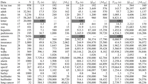
Table 1: The search timeT, the number of collected networks|G|and the number of MECs|M|in the collected networks at BF = 3, 20 and 150 using BIC, wherenis the number of random variables in the dataset,N is the number of instances in the dataset and OT = Out of Time.

collects more networks in a shorter period of time. With the pruning rules generalized above, our method can scale up to datasets with 57 variables in BIC scoring, whereas the pre-vious best results are reported on a network of 29 variables using thek-best approach with score pruning (Chen, Dar-wiche, and Choi 2018).

The datasets are obtained from the UCI Machine Learn-ing Repository (Dheeru and Karra Taniskidou 2017) and the Bayesian Network Repository2_{. Some of the complete local}

scoring files are downloaded from the GOBNILP website3 and are used for thek-best related experiments only. Since not all solvers in thek-best experiments can take in scoring files, we exclude the time to compute local scores from the comparison. Both BIC/MDL (Schwarz 1978, Lam and Bac-chus 1994) and BDeu (Buntine 1991, Heckerman, Geiger, and Chickering 1995) scoring functions are used where ap-plicable. All experiments are conducted on computers with 2.2 GHz Intel E7-4850V3 processors. Each experiment is limited to 64 GB of memory and 24 hours of CPU time.

The Bayes Factor Approach

We modified the development version (9c9f3e6) of GOB-NILP, referred below as GOBNILP dev, to apply pruning rules presented above during scoring and supplied

appropri-2

http://www.bnlearn.com/bnrepository/ 3

https://www.cs.york.ac.uk/aig/sw/gobnilp/#benchmarks

ate parameter settings for collecting near-optimal networks4_.

The code is compiled with SCIP 6.0.0 and CPLEX 12.8.0. GOBNILP extends the SCIP Optimization Suite (Gleixner et al. 2018) by adding aconstraint handlerfor handling the acyclicity constraint for DAGs. If multiple BNs are required GOBNILP dev just calls SCIP to ask it to collect feasible solutions. In this mode, when SCIP finds a solution, the so-lution is stored, a constraint is added to render that soso-lution infeasible and the search continues. This differs from (and is much more efficient than) GOBNILP’s current method for findingk-best BNs where an entirely new search is started each time a new BN is found. A recent version of SCIP has a separate “reoptimization” method which might allow bet-terk-best performance for GOBNILP but we do not explore that here. By default when SCIP is asked to collect solutions it turns off all cutting plane algorithms. This led to very poor GOBNILP performance since GOBNILP relies on cutting plane generation. Therefore, this default setting is overrid-den in GOBNILP dev to allow cutting planes when collect-ing solutions. To find only solutions with objective no worse than (OPT +), SCIP’sSCIPsetObjlimitfunction is used. Note that, for efficiency reasons, this isnoteffected by adding a linear constraint.

We first use GOBNILP dev to find the optimal scores since GOBNILP dev takes objective limit (OPT +) for enumerating feasible networks. Then all networks falling

4

Data n N Tk(s) k TEC(s) |Gk| T20(s) |G20| |M20|

tic tac toe 10 958

0.2 10 0.5 67

0.6 152 24

2.8 100 6.0 673

70.7 1,000 78.5 7,604

wine 14 178

3.4 10 12.0 60

35.9 8,734 6,262

85.0 100 168.4 448

3,420.4 1,000 3,064.4 4,142

adult 14 32,561

3.3 10 633.5 68

9.3 792 19

73.6 100 63,328.9 1,340

2,122.8 1,000 OT —

nltcs 16 3,236

11.8 10 47,338.4 552

125.5 652 326

406.6 100 OT —

13,224.6 1,000 OT —

msnbc 17 58,265 ES — ES — 4,018.9 24 24

letter 17 20,000

26.0 10 18,788.0 200

56,344.8 20 10

909.8 100 OT —

41,503.9 1,000 OT —

voting 17 435

34.1 10 101.9 30

6.0 621 207

1,125.7 100 1,829.2 3,392

38,516.2 1,000 42,415.3 3,665

zoo 17 101

33.5 10 99.8 52

8,418.8 29,073 6,761

1,041.7 100 1,843.4 100

41,412.1 1,000 OT —

hepatitis 20 155

351.2 10 872.3 89

441.4 28,024 3,534

13,560.3 100 20,244.7 842

OT 1,000 OT —

parkinsons 23 195

3,908.2 10 OT —

1,515.9 150,000 42,448

OT 100 OT —

OT 1,000 OT —

autos 26 159 OM 1 OM — OT — —

insurance 27 1,000 OM 1 OM — 8.3 1,081 133

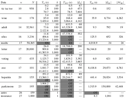
Table 2: The search timeTand the number of collected networksk,|Gk|and|G20|for KBest, KbestEC and GOBNILP dev (BF = 20) using BDeu, wherenis the number of random variables in the dataset,N is the number of instances in the dataset, OM = Out of Memory, OT = Out of Time and ES = Error in Scoring. Note that|Gk|is the number of DAGs covered by thek-best

MECs in KBestEC and|M20|is the number of MECs in the networks collected by GOBNILP dev.

into the limit are collected with a counting limit of 150,000. Finally the collected networks are categorized into Markov equivalence classes (MECs), where two networks belong to the same MEC iff they have the same skeleton and v-structures (Verma and Pearl 1990). The proposed approach is tested on datasets with up to 57 variables. The search time T, the number of collected networks|G|and the number of MECsMin the collected networks at BF = 3, 20 and 150 using BIC are reported in Table 1, wherenis the number of random variables in the dataset andN is the number of instances in the dataset. The three thresholds are chosen ac-cording to the interpreting scale suggested by (Heckerman, Geiger, and Chickering 1995) where 3 marks the difference between anecdotal and positive evidence, 20 marks positive and strong evidence and 150 marks strong and very strong evidence. The search time mostly depends on a combined effect of the size of the network, the sample size and the number of MECs at a given BF. Some fairly large networks such as alarm, sponge and barley are solved much faster than smaller networks with a large sample size, e.g., msnbc and letter.

The results also indicate that the number of collected

net-works and the number of MECs at three BF levels varies substantially across different datasets. In general, datasets with smaller sample sizes tend to have more networks col-lected at a given BF since near-optimal networks have simi-lar posterior probabilities to the best network. Although the desired level of BF for a study, like the p-value, is often de-termined with domain knowledge, the proposed approach, given sufficient samples, will produce meaningful results that can be used for further analysis.

Bayes Factor vs.

k

-Best

In this section, we compare our approach with published solvers that are able to find a subset of top-scoring net-works with the given parameter k. The solvers under con-sideration are KBest 12b5 from (Tian, He, and Ram 2010), KBestEC6_{from (Chen and Tian 2014), and GOBNILP 1.6.3}

(Bartlett and Cussens 2013), referred to as KBest, KBestEC and GOBNILP below. The first two solvers are based on the dynamic programming approach introduced in (Silander and

5

http://web.cs.iastate.edu/∼_{jtian/Software/UAI-10/KBest.htm} 6

http://web.cs.iastate.edu/∼_{jtian/Software/AAAI-14-yetian/}

Myllym¨aki 2006). Due to the lack of support for BIC in KBest and KBestEC, only BDeu with a equivalent sample size of one is used in corresponding experiments.

The most recent stable version of GOBNILP is 1.6.3 that works with SCIP 3.2.1. The default configuration is used and experiments are conducted for both BIC and BDeu scor-ing functions. However, thek-best results are omitted here due to its poor performance. Despite that GOBNILP can it-eratively find the k-best networks in descending order by adding linear constraints, the pruning rules designed to find the best network are turned off to preserve sub-optimal net-works. In fact, the memory usage often exceeded 64 GB dur-ing the initial ILP formulation, indicatdur-ing that the lack of pruning rules posed serious challenge for GOBNILP. GOB-NILP dev, on the other hand, can take advantage of the prun-ing rules presented above in the proposed BF approach and its results compare favorably to KBest and KBestEC.

The experimental results of KBest, KBestEC and GOB-NILP dev are reported in Table 2, wheren is the number of random variables in the dataset,N is the number of in-stances in the dataset, andk is the number of top scoring networks. The search timeTis reported for KBest, KBestEC and GOBNILP dev (BF = 20). The number of DAGs cov-ered by thekMECs|Gk|is reported for KBestEC. In

com-parison, the last two columns are the number of found net-works|G20|and the number of MECs|M20|using the BF approach with a given BF of 20 and BDeu scoring function. As the number of requested networks k increases, the search time for both KBest and KBestEC grows exponen-tially. The KBest and KBestEC are designed to solve prob-lems of size fewer than 207, and so they have some difficulty with larger datasets. They also fail to generate correct scor-ing files for msnbc. KBestEC seems to successfully expand the coverage of DAGs with some overhead for checking equivalence classes. However, KBestEC took much longer than KBest for some instances, e.g., nltcs and letter, and the number of DAGs covered by the found MECs is inconsis-tent for nltcs, letter and zoo. The search time for the BF approach is improved over thek-best approach except for datasets with very large sample sizes. The generalized prun-ing rules are very effective in reducprun-ing the search space, which then allows GOBNILP dev to solve the ILP problem subsequently. Comparing to the improved results in (Chen, Choi, and Darwiche, 2015; 2016), our approach can scale to larger networks if the scoring file can be generated.8

Now we show that different datasets have distinct score patterns in the top scoring networks. The scores of the 1,000-best networks for some datasets in the KBest experiment are plotted in Figure 2. A specific line for a dataset indicates the deviationfrom the optimal BDeu score by thekth-best network. For reference, the red dash lines represent different levels of BFs calculated by = logBF (See Equation 3). The figure shows that it is difficult to pick a value forka priorito capture the appropriate set of top scoring networks. For a few datasets such as adult and letter, it only takes fewer

7

Obtained through correspondence with the author. 8

We are unable to generate BDeu score files for datasets with over 30 variables.

Figure 2: The deviationfrom the optimal BDeu score byk using results from KBest. The corresponding values of the BF ( = log(BF), see Equation 3) are presented on the right. For example, if the desired BF value is 20, then all networks falling below the dash line at 20 are credible.

than 50 networks to reach a BF of 20, whereas zoo needs more than 10,000 networks. The sample size has a signifi-cant effect on the number of networks at a given BF since the lack of data leads to many BNs with similar probabili-ties. It would be reasonable to choose a large value forkin model averaging when data is scarce and vice versa, but only the BF approach is able to automatically find the appropriate and credible set of networks for further analysis.

Conclusion

References

Bartlett, M., and Cussens, J. 2013. Advances in Bayesian network learning using integer programming. In Proceed-ings of the 29th Conference on Uncertainty in Artificial In-telligence, 182–191.

Buntine, W. L. 1991. Theory refinement of Bayesian net-works. InProceedings of the Seventh Conference on Uncer-tainty in Artificial Intelligence, 52–60.

Chen, Y., and Tian, J. 2014. Finding thek-best equivalence classes of Bayesian network structures for model averaging. InProceedings of the 28th Conference on Artificial Intelli-gence, 2431–2438.

Chen, E. Y.-J.; Choi, A.; and Darwiche, A. 2015. Learning Bayesian networks with non-decomposable scores. In Pro-ceedings of the 4th IJCAI Workshop on Graph Structures for Knowledge Representation and Reasoning (GKR 2015), 50– 71. Available as: LNAI 9501.

Chen, E. Y.-J.; Choi, A.; and Darwiche, A. 2016. Enumer-ating equivalence classes of Bayesian networks using EC graphs. InProceedings of the 19th International Conference on Artificial Intelligence and Statistics (AISTATS), 591–599. Chen, E. Y.-J.; Darwiche, A.; and Choi, A. 2018. On pruning with the MDL score. International Journal of Approximate Reasoning92:363–375.

Claeskens, G., and Hjort, N. L. 2008. Model Selection and Model Averaging. Cambridge University Press.

Cussens, J., and Bartlett, M. 2012. GOBNILP 1.2 user/developer manual.University of York, York.

Darwiche, A. 2009.Modeling and Reasoning with Bayesian Networks. Cambridge University Press.

Dash, D., and Cooper, G. F. 2004. Model averaging for prediction with discrete Bayesian networks. Journal of Ma-chine Learning Research5:1177–1203.

de Campos, C. P., and Ji, Q. 2011. Efficient structure learn-ing of Bayesian networks uslearn-ing constraints.J. Mach. Learn. Res.12:663–689.

de Campos, C. P.; Scanagatta, M.; Corani, G.; and Zaffalon, M. 2018. Entropy-based pruning for learning Bayesian net-works using BIC.Artificial Intelligence260:42–50. Dheeru, D., and Karra Taniskidou, E. 2017. UCI machine learning repository.

Gleixner, A.; Bastubbe, M.; Eifler, L.; Gally, T.; Gam-rath, G.; Gottwald, R. L.; Hendel, G.; Hojny, C.; Koch, T.; L¨ubbecke, M. E.; Maher, S. J.; Miltenberger, M.; M¨uller, B.; Pfetsch, M. E.; Puchert, C.; Rehfeldt, D.; Schl¨osser, F.; Schubert, C.; Serrano, F.; Shinano, Y.; Viernickel, J. M.; Walter, M.; Wegscheider, F.; Witt, J. T.; and Witzig, J. 2018. The SCIP Optimization Suite 6.0. Technical report, Opti-mization Online.

He, R.; Tian, J.; and Wu, H. 2016. Bayesian learning in Bayesian networks of moderate size by efficient sampling. Journal of Machine Learning Research17:1–54.

Heckerman, D.; Geiger, D.; and Chickering, D. M. 1995. Learning Bayesian networks: The combination of knowl-edge and statistical data.Machine Learning20:197–243.

Hoeting, J. A.; Madigan, D.; Raftery, A. E.; and Volinsky, C. T. 1999. Bayesian model averaging: A tutorial.Statistical Science14(4):382–401.

Jeffreys, S. H. 1967. Theory of Probability: 3d Ed. Claren-don Press.

Kass, R. E., and Raftery, A. E. 1995. Bayes factors.Journal of the American Statistical Association90(430):773–795. Koivisto, M., and Sood, K. 2004. Exact Bayesian struc-ture discovery in Bayesian networks. J. Mach. Learn. Res. 5:549–573.

Koller, D., and Friedman, N. 2009. Probabilistic Graphical Models: Principles and Techniques. The MIT Press. Lam, W., and Bacchus, F. 1994. Using new data to refine a Bayesian network. InProceedings of the Tenth Conference on Uncertainty in Artificial Intelligence, 383–390.

Madigan, D., and Raftery, A. E. 1994. Model selection and accounting for uncertainty in graphical models using Occam’s window. Journal of the Amercian Statistical As-sociation89:1535–1546.

Meil˘a, M., and Jaakkola, T. 2000. Tractable Bayesian learn-ing of tree belief networks. InProceedings of the 16th Con-ference on Uncertainty in Artificial Intelligence, 380–388. Ripley, B. D. 1996. Pattern recognition and neural networks. Cambridge University Press.

Schwarz, G. 1978. Estimating the dimension of a model. The Annals of Statistics6:461–464.

Silander, T., and Myllym¨aki, P. 2006. A simple approach for finding the globally optimal Bayesian network structure. In Proceedings of the 22nd Conference on Uncertainty in Artificial Intelligence, 445–452.

Teyssier, M., and Koller, D. 2005. Ordering-based search: A simple and effective algorithm for learning Bayesian net-works. In Proceedings of the 21st Conference on Uncer-tainty in Artificial Intelligence, 548–549.

Tian, J.; He, R.; and Ram, L. 2010. Bayesian model aver-aging using the k-best Bayesian network structures. In Pro-ceedings of the 26th Conference on Uncertainty in Artificial Intelligence, 589–597.