Block Belief Propagation for Parameter Learning in Markov Random Fields

(1)

The Thirty-Third AAAI Conference on Artificial Intelligence (AAAI-19)

Block Belief Propagation for Parameter Learning in Markov Random Fields

You Lu

Department of Computer Science Virginia Tech

Blacksburg, VA [email protected]

Zhiyuan Liu

Department of Computer Science University of Colorado Boulder

Boulder, CO [email protected]

Bert Huang

Department of Computer Science Virginia Tech

Blacksburg, VA [email protected]

Abstract

Traditional learning methods for training Markov random fields require doing inference over all variables to compute the likelihood gradient. The iteration complexity for those methods therefore scales with the size of the graphical mod-els. In this paper, we proposeblock belief propagation learn-ing(BBPL), which uses block-coordinate updates of approx-imate marginals to compute approxapprox-imate gradients, removing the need to compute inference on the entire graphical model. Thus, the iteration complexity of BBPL does not scale with the size of the graphs. We prove that the method converges to the same solution as that obtained by using full inference per iteration, despite these approximations, and we empiri-cally demonstrate its scalability improvements over standard training methods.

Introduction

Markov random fields (MRFs) and conditional random fields (CRFs) are powerful classes of models for learning and inference of factored probability distributions (Koller and Friedman 2009; Wainwright and Jordan 2008). They have been widely used in tasks such as structured pre-diction (Taskar, Guestrin, and Koller 2004) and computer vision (Nowozin and Lampert 2011). Traditional training methods for MRFs learn by maximizing an approximate maximum likelihood. Many such methods use variational in-ference to approximate the crucial partition function.

With MRFs, the gradient of the log likelihood with respect to model parameters is the marginal vector. With CRFs, it is the expected feature vector. These identities suggest that each iteration of optimization must involve computation of the full marginal vector, containing the estimated marginal probabilities of all variables and all dependent groups of variables. In some applications, the number of variables can be massive, making traditional, full-inference learning too expensive in practice. This problem limits the application of MRFs in modern data science tasks.

In this paper, we proposeblock belief propagation learn-ing(BBPL), which alleviates the cost of learning by comput-ing approximate gradients with inference over only a small block of variables at a time. BBPL first separates the Markov

network into several small blocks. At each iteration of learn-ing, it selects a block and computes its marginals. It approx-imates the gradient with a mix of the updated and the previ-ous marginals, and it updates the parameters of interest with this gradient.

Related Work

Many methods have been developed to learn MRFs. In this section, we cover only the BP-based methods.

Mean-field variational inference and belief propagation (BP) approximate the partition function with non-convex entropies, which break the convexity of the original par-tition function. In contrast, convex BP (Globerson and Jaakkola 2007; Heskes 2006; Schwing et al. 2011; Wain-wright, Jaakkola, and Willsky 2005; Wainwright 2006) pro-vides a strongly convex upper bound for the partition func-tion. This strong convexity has also been theoretically shown to be beneficial for learning (London, Huang, and Getoor 2015). Thus, our BBPL method uses convex BP to approxi-mate the partition function.

Regarding inference, some methods are developed to ac-celerate computations of the beliefs and messages. Stochas-tic BP (Noorshams and Wainwright 2013) updates only one dimension of the messages at each inference iteration, so its iteration complexity is much lower than traditional BP. Distributed BP (Schwing et al. 2011; Yin and Gao 2014) distributes and parallelizes the computation of beliefs and messages on a cluster of machines to reduce inference time. Sparse-matrix BP (Bixler and Huang 2018) uses sparse-matrix products to represent the message-passing indexing, so that it can be implemented on modern hardware. How-ever, to learn MRF parameters, we need to run these infer-ence algorithms for many iterations on the whole network until convergence at each parameter update. Thus, these methods are still impacted by the network size.

(2)

in-ference on the full network for a fixed number of iterations or until convergence. Moreover, they yield non-convex ob-jectives without convergence guarantees.

Some methods restrict the complexity of inference on a subnetwork at each parameter update. Lifted BP (Kersting, Ahmadi, and Natarajan 2009; Singla and Domingos 2008) makes use of the symmetry structure of the network to group nodes into super-nodes, and then it runs a modified BP on this lifted network. A similar approach (Ahmadi, Kersting, and Natarajan 2012) uses a lifted online training framework that combines the advantages of lifted BP and stochastic gra-dient methods to train Markov logic networks (Richardson and Domingos 2006). These lifting approaches rely on sym-metries in relational structure—which may not be present in many applications—to reduce computational costs. They also require extra algorithms to construct the lifted network, which increase the difficulty of implementation. Piecewise training separates a network into several possibly overlap-ping sets of pieces, and then uses the piecewise pseudo-likelihood as the objective function to train the model (Sut-ton and McCallum 2009). Decomposed learning (Samdani and Roth 2012) uses a similar approach to train structured support vector machines. However, these methods need to modify the structure of the network by decomposing it, thus changing the objective function.

Finally, inner-dual learning methods (Bach et al. 2015; Hazan and Urtasun 2010; Hazan, Schwing, and Urtasun 2016; Meshi et al. 2010; Taskar et al. 2005) interleave pa-rameter optimization and inference to avoid repeated infer-ences during training. These methods are fast and conver-gent in many settings. However, in other settings, key bot-tlenecks are not fully alleviated, since each partial inference still runs on the whole network, causing the iteration cost to scale with the network size.

Contributions

In contrast to many existing approaches, our proposed method uses the same convex inference objective as tradi-tional learning, providing the same benefits from learning with a strongly convex objective. BBPL thus scales well to large networks because it runs convex BP on a block of vari-ables, fixing the variables in other blocks. This block up-date guarantees that the iteration complexity does not in-crease with the network size. BBPL preserves communica-tion across the blocks, allowing it to optimize the original objective that computes inference over the entire network at convergence. The update rules of BBPL are similar in form to full BP learning, which makes it as easy to implement as traditional MRF or CRF training. Finally, we theoretically prove that BBPL converges to the same solution under mild conditions defined by the inference assumption. Our exper-iments empirically show that BBPL does converge to the same optimum as full BP.

Background

In this section, we introduce notation and background knowledge directly related to our work.

Convex Belief Propagation for MRFs

Let x = [x1, ..., xn] be a discrete random vector taking

values in X = X1 × · · · × Xn, and let G = (V, E) be the corresponding undirected graph, with the vertex set

V ={1, ..., n}and edge setE⊂V×V. Potential functions

θs : Xs → Randθuv : Xu× Xv → Rare differentiable

functions with parameters we want to learn. The probability density function of a pairwise Markov random field (Wain-wright and Jordan 2008) can be written as

p(x|θ) = exp{X

s∈V

θs(xs) +

X

(u,v)∈E

θuv(xu, xv)−A(θ)}.

The log partition function

A(θ) = logX

X

exp{X

s∈V

θs(xs) +

X

(u,v)∈E

θuv(xu, xv)}

(1) is intractable in most situations whenGis not a tree. One can approximate the log partition function with a convex upper bound:

B(θ) = max

τ∈L(G){h

θ, τi −B∗(τ)}, (2)

where

θ = {θs|s∈V} ∪ {θuv|(u, v)∈E}, τ = {τs|s∈V} ∪ {τuv|(u, v)∈E},

L(G) := {τ∈Rd+|

X

xs

τs(xs) = 1,

X

xv

τuv(xu, xv) =τu(xu)}.

The vectorτ is called the pseudo-marginal or belief vec-tor. Specifically,τsis the unary belief of vertexs, andτuvis

the pairwise belief of edge(u, v). Thelocal marginal poly-topeLrestricts the unary beliefs to be consistent with their

connected pairwise beliefs. We consider a variant of belief propagation whereB∗(τ)is strongly convex and has the fol-lowing form:

B∗(τ) = X

s∈V

ρsH(τs) +

X

(u,v)∈E

ρuvH(τuv),

whereρsandρuv are parameters known as counting

num-bers, andH(.)is the entropy.

Equation 2 can be solved via convex BP (Meshi et al. 2009; Yedidia, Freeman, and Weiss 2005). Letλuv be the

message from vertexuto vertexv. The update rules of mes-sages and beliefs are as follows:

λuv =ρuvlog

X

u

exp{ 1

ρuv

(θuv−λvu) + logτu}, (3)

where

τu∝exp{

1

ρu

(θu+

X

v∈N(u)

λvu)}, (4)

and

τuv ∝ exp{

1

ρuv

(3)

Other forms of convex BP, such as tree-reweighted BP (Wainwright, Jaakkola, and Willsky 2005), can also be used in our approach. Convex BP does not always converge on loopy networks. However, under some mild conditions, it is guaranteed to converge and can be a good approxima-tion for general networks (Roosta, Wainwright, and Sastry 2008).

Learning Parameters of MRFs

In this subsection, we introduce traditional training methods for fitting MRFs to a dataset via a combination of BP and a gradient-based optimization. The learning algorithm is given a dataset withNdata points, i.e.,w1, ..., wN. It then learns θby minimizing the negative log-likelihood:

L(θ) = −1 N

X

n

logp(wn|θ)

= −1

N

X

n

θTwn+A(θ)

≈ −θTw¯+B(θ)

= −θTw¯+ max

τ∈L(G){hθ, τi −B

∗₍_τ₎_}_, ₍₆₎

wherew¯= 1/NP

nwn.

UsingB(θ)as the tractable approximation ofA(θ), the traditional learning approach is to minimize L(θ) using gradient-based methods. Letθt be the parameter vector at

iterationt, and letτ_t∗be the optimizedτ corresponding to

θt. Then gradient learning is done by iterating

θt+1=θt−αt∇θL(θt), (7)

where

∇θL(θt) =−w¯+τt∗, (8)

andαtis the learning rate. The traditional parameter

learn-ing process is described in Algorithm 1.

Algorithm 1Parameter learning with full convex BP

1: Initializeθ0.

2: Whileθhas not converged 3: Whileλhas not converged 4: Updateτwith Equation 4. 5: Updateλwith Equation 3. 6: end

7: ∇L(θt) =−w¯+τt∗

8: θt+1=θt−αt∇L(θt)

9: end

Traditional parameter learning requires running inference on each full training example per gradient update, so we re-fer to it asfull BP learning. These full inferences cause it to suffer scalability limitations when the training data includes large MRFs. The goal of our contributions is to circumvent these limitations.

Block Belief Propagation Learning

In this section, we introduce our proposed method, which has a much lower iteration complexity than full BP learning and is guaranteed to converge to the same optimum as full convex BP learning.

Algorithm Description

The full BP learning method in Algorithm 1 does not scale well to large networks. It needs to perform inference on the full network at each iteration, i.e., Step 2 to Step 5 in Al-gorithm 1. The iteration complexity depends on the size of network. When the network is large—e.g., a network with at least tens of thousands of nodes—the dimensions ofτandλ

are also large. Updating all their dimensions in each gradient step creates a significant computational inefficiency.

To address this problem, we developblock belief propaga-tion learning(BBPL). BBPL only needs to do inference on a subnetwork at each iteration, which means that, for tem-plated models, the iteration complexity of BBPL does not depend on the size of the network. For non-templated mod-els, the iteration complexity has a greatly reduced depen-dency on the network size. Moreover, we can prove the con-vergence of BBPL, guaranteeing that it will converge to the same optimum as full BP learning. Finally, BBPL’s update rules are analogous to those of full BP learning, so it is as easy to implement as full BP learning.

BBPL first separates the vertex set V into D subsets

V1, ..., VD. Then it separates the edge setE intoDsubsets

of edges incident on the corresponding vertex subsets, i.e.,

Ei = {(u, v)|(u, v)∈ E and (u ∈ Vi or v ∈ Vi)}.

Thus, we have that V = V1∪V2 ∪...∪VD, and E = E1∪E2∪...∪ED. For shorthand, letFi = (Ei, Vi)

de-note theith subnetwork.

At iterationt, BBPL selects a subgraphFiand only

up-dates eachτuifu∈Vi, andτuvand onlyλuvif(u, v)∈Ei.

It updates this block of messages and beliefs via belief propagation—i.e., Equations 3, 4, and 5—holding all other messages and beliefs fixed until convergence. Finally, BBPL uses the updated block of beliefs to updateθby computing an approximate gradient. Our empirical results show that ei-ther selecting subgraphs randomly or sequentially can lead to convergence, but sequentially selecting subgraphs can make the algorithm converge faster.

With a slight abuse of notation, let Ft be the

subnet-work selected at iterationt. Letτ_t(Ft)andλ(_tFt)be the sub-matrices ofτtandλt, respectively, that correspond toFt. Let UFt be a projection matrix that projects the parameter from

R|Ft|toRd. The update rules forτtandλtare

τt=τt−1+UFt(τ

(Ft) t −τ

(Ft)

t−1), (9) and

λt=λt−1+UFt(λ

(Ft)

t −λ

(Ft)

t−1). (10) After computingτtandλt, BBPL updates the parameters

using the approximate gradient:

g(θt) =−w¯+τt. (11)

Note that the only difference betweeng(θt)andg(θt−1)is the term τ(Ft)

t −τ

(Ft)

t−1. Thus, given g(θt−1), we can effi-ciently update our gradient estimate with

g(θt) =g(θt−1) +UFt(τ

(Ft) t −τ

(Ft) t−1).

(4)

gradient at the entries where the block marginal update was performed can be done in place. Thus, the complexity of the whole inference process and gradient computation depends only on the size of the subnetwork. The only step that re-quires time complexity that scales with the network size is the actual parameter update using the gradient, which we will later alleviate when using templated models. The com-plete algorithm is listed in Algorithm 2.

Algorithm 2Parameter estimation with block BP

1: SeparategintoM subnetwork, i.e.,F1, ..., FM.

2: Whileθhas not converged 3: Select a subgraphFt.

4: WhileλFt_{has not converged}

5: Updateτ_tFtwith Equation 4. 6: UpdateλFt

t with Equation 3.

7: end

8: g(θt) =g(θt−1) +UFt(τ

(Ft) t −τ

(Ft) t−1). 9: θ(t+1)=θ(t)−αtg(θt).

10: end

Convergence Analysis

In this subsection, we theoretically prove the convergence of BPPL. We first rewrite the learning problem as follows:

min

θ τmax∈L(G)

−θTw¯+θTτ−B∗(τ). (12)

Equation 12 is a convex-concave saddle-point problem. We use(θ∗, τ∗)to represent its saddle point. Its correspond-ing primal problem is

min

θ L(θ) =−θ

T_w_¯₊_B₍_θ₎_, ₍₁₃₎

whereB(θ)is defined in Equation 2. Equation 12 and Equa-tion 13 have the same optimalθ.

Thus, we can prove the convergence of BBPL follow-ing the general framework for provfollow-ing the convergence of saddle-point optimizations (Du and Hu 2018). We prove that under a mild assumption, i.e., Assumption 1, BBPL has a linear convergence rate.

Assumption 1 Whenθhas not converged, the block

coordi-nate update, i.e., Equation 9, satisfies the following inequal-ity:

||τt+1−τt∗+1|| ≤(1−c)||τt−τt∗+1||, where0< c <1.

Informally, we can interpret Assumption 1 to mean that, at iterationt+ 1, the vectorτt+1with new blockτ

(Ft) t+1 will get closer to the optimumτt∗+1. This assumption is easy to

satisfy whenθhas not converged. Since the blockτ_t(₊₁Ft)of

τt+1 is updated with respect toθt+1, andτt∗+1 is the true optimum with respect toθt+1,τt+1should be closer toτt∗+1. Whenθ converges, block BP becomes a block coordinate update method. Based on claims shown by Schwing et al. (2011),τtconverges toτ∗.

The following theorem establishes the linear convergence guarantee of Algorithm 2.

Theorem 1 The primal of BBPL, i.e., Equation 13, is β

-strongly convex andη-smooth. When we use BBPL to learn the parameters, suppose BBPL satisfies Assumption 1. De-fine the Lyapunov function

Pt=||θt−θ∗||+γ||τt−τt∗||.

When0< αt≤min{₂_η2₊cβ_ηβ₊_β2,

2

η+β}, andγ= β

2(1−c)η2,

we have

Pt+1 ≤(1−δ)Pt,

where0 < δ <1. This bound implies thatlimt→∞Pt= 0,

andθtwill converge linearly to the optimumθ∗.

Proof sketch.The proof is based on the proof framework detailed by Du and Hu (2018). The proof can be divided to three steps. First, we bound the decrease of ||θt−θ∗||.

Second, we bound the decrease of||τt−τ_t∗||. Third, we prove that Pt+1 ≤ (1−δ)Pt. The complete proof is in the long

version of this paper (Lu, Liu, and Huang 2018).

Generalization to Templated or Conditional

Models

So far, we have described the BBPL approach in the set-ting where there is a separate parameter for every entry in the marginal vector. In templated or conditional models, the parameters can be shared across multiple entries. We de-scribe here how BBPL generalizes to such models. For con-ditional models, we use MRFs to infer the probability of out-put variablesY given input variablesX, i.e.,Pr(Y|X). A standard modeling technique for this task is to encode the joint states of the input and output variables with some fea-ture vectors, so the parameters are weights for these feafea-tures. We are given a dataset of fully observed input-output pairs

S ={(Mi, yi)}iN=1, whereMi ∈ RK×dis the feature

ma-trix, andyi∈Rdis the label vector (i.e., the one-hot

encod-ing of the ground-truth variable states). The negative log-likelihood of a conditional random field is defined as

L(˜θ) =−1 N

N

X

i=1

logLi(˜θ, Mi, yi), (14)

whereθ˜∈RKis the parameter we want to learn, and

Li(˜θ, Mi, yi) = ˜θTMiyi−B(˜θTMi). (15)

The definition ofB(˜θTMi)is similar to that for MRFs.

We can interpretθ˜>Mito be the expanded, or “grounded,”

potential vector. The product with feature matrixMimaps

from the low-dimensionalθ˜to a possibly high-dimensional, full potential vectorθ. To be precise, the definition is

B(˜θTMi) = max

τi∈L(G){

˜

θTMiτi−B∗(τi)}.

For each data point i, we can still use BBP to update

τi,t at iteration t, i.e, lines 4–9 in Algorithm 2. Let w¯ =

1

N

P

iMiyi. The approximate gradient is then

g( ˜θt) = ¯w−

1

N N

X

i=1

(5)

Giveng(˜θt−1), we computeg(˜θt)with the following rule:

g(˜θt−1) =g(˜θt−1) +

1

N N

X

i=1

Ui,Ft(τ

(Ft) i,t −τ

(Ft) i,t−1).

Thus, the iteration complexity of inference only depends on the subnetwork size, rather than the size of the whole network.

Regarding convergence, note that each matrixMiis

con-stant, and its norm is bounded by its eigenvalues. Using the same proof method as that of Theorem 1, we can straight-forwardly prove that it still has a linear convergence rate.

The same formulation—using a matrixM to map from a low-dimensional parameter vector θ˜to a possibly high-dimensional, full potential vector—can also be used to de-scribe templated MRFs, where the same potential func-tions may be used in multiple parts of the graph. Therefore the same techniques and analysis also apply for templated MRFs.

Empirical Study

In this section, we empirically analyze the performance of BBPL. We design two groups of experiments. In the first group of experiments, we evaluate the sensitivity of our method on the block size and empirically measure its con-vergence on synthetic networks. In the second group of ex-periments, we test our methods on a popular application of MRFs: image segmentation on a real image dataset.

Baselines We compare BBPL to other methods that

ex-actly optimize the full variational likelihood. We use full convex BP and inner-dual learning (Bach et al. 2015; Hazan, Schwing, and Urtasun 2016) as our baselines. Full BP learn-ing runs inference to convergence each gradient step, and inner-dual learning accelerates learning by performing only one iteration of inference per learning iteration.

Metrics We evaluate the convergence and correctness of

our method by measuring the objective value and the dis-tance between the current parameter vectorθand the optimal

θ∗_{. To compute the objective value, we store the parameters} θtobtained by full BP learning, BBPL, or inner-dual

learn-ing durlearn-ing trainlearn-ing. We then plug each into Equation 15 to compute the variational negative log-likelihood. To compute the distance betweenθtandθ∗, we first run convex BP

learn-ing until convergence to getθ∗, and then we use the`2norm to measure the distance.

Experiments on Synthetic Networks

We generate two types of synthetic MRFs: grid networks and Barab´asi-Albert (BA) random graph networks (Albert and Barab´asi 2002). The nodes of the BA networks are or-dered according to their generating sequence. We gener-ate true unary and pairwise features from zero-mean, unit-variance Gaussian distributions. The unary feature dimen-sion is 20 and the pairwise feature dimendimen-sion is 10, and each variable has 8 possible states. Once the true models are gen-erated, we draw 20 samples for each dataset with Gibbs sam-pling.

●

● ● ● ● ● ● ● ● ● ● ● ● ● ●

Grid Network

1x5 2x5 3x5 4x5 5x5 5x6 5x7 5x8 5x9 5x10 6x10 7x10 8x10 9x10 10x10 0

2000 4000 6000

Running Time (s)

Network Size

● _100x100 150x150 200x200 50x50

● ● ● ● ● ● ● ● ● ● ● ● ● ● ●

BA Network

25 50 75 100

0 1000 2000 3000 4000

Number of Blocks

Network Size

● _{1000 Nodes} 10000 Nodes 20000 Nodes 5000 Nodes

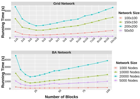
Figure 1: Sensitivity of BBPL to block size. The label5×5

in the top polot represents that each grid is divided to 5 rows and 5 columns of sub-networks. The label20in the bottom plot represents that the network is divided into 20 networks. The results show that BBPL converges the fastest when each block’s size is about20to25times smaller than the network.

Sensitivity to block size We conduct experiments on grid

networks of four different sizes, i.e., 50×50,100×100,

150×150, and200×200, and on BA networks with four different sizes, i.e., 1,000 nodes, 5,000 nodes, 10,000 nodes, and 20,000 nodes. For the grid networks, we vary the num-ber of blocks from25 (5×5)to100 (10×10). For example, when the network size is200×200and the number of blocks is5×5, we separate the network into25sub-networks, and each sub-network’s size is40×40. For the BA networks, we vary the number of blocks from5to100. We separate the nodes of each BA network based on their indices. For example, for a node set V = {1,2, ...,10}, if we want to separate it into two subsets, we will letV1 = 1, ...,5, and

V2={6, ...,10}.

The results are plotted in Figure 1. The trends indicate that when each block is between20to25times smaller than the network, BBPL converges the fastest. When the block size is too small, the algorithm needs more iterations to converge. When the block size is too large, per-iteration complexity will be large. Blocks that are either too large or too small can reduce the benefits of BBPL.

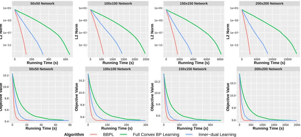
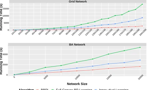
Convergence analysis For the grid networks, we vary the

network size from 10×10 to200×200, and we set the number of blocks to4×5. For the BA networks, we vary the network size from100to 20,000, and we set the number of blocks to20. Figure 2 and Figure 3 empirically show the convergence of BBPL on different networks. Figure 4 plots the running time comparison on networks with all sizes. From Figure 2 we can see that BBPL converges to the same solution as full BP learning, while requiring significantly less time. Figure 4 shows that on all networks, BBPL is the fastest. The acceleration is more significant when the net-work is large. For example, when the grid netnet-work’s size is

(6)

inner-50x50 Network

0 200 400 600

1e−11 1e−07 1e−03 1e+01

L2 Norm

100x100 Network

0 500 1000 1500 2000 2500 1e−11

1e−07 1e−03 1e+01

L2 Norm

150x150 Network

0 2000 4000 6000 8000 1e−11

1e−07 1e−03 1e+01

L2 Norm

200x200 Network

0 5000 10000 15000 1e−11

1e−07 1e−03 1e+01

L2 Norm

50x50 Network

0 20 40 60 80

9.4 9.6 9.8 10.0 10.2

Objective V

alue

100x100 Network

0 100 200 300

9.6 9.8 10.0 10.2

Objective V

alue

150x150 Network

0 300 600 900

9.6 9.8 10.0 10.2

Objective V

alue

200x200 Network

0 500 1000 1500 2000 2500 9.6

9.8 10.0 10.2

Objective V

alue

Algorithm BBPL Full Convex BP Learning Inner−dual Learning

Figure 2: Convergence on grid networks. The top row plots the`2distance from the optimum, and the second row plots the objective values. The`2plots show the full running time of each method, but for clarity, we zoom into the plots of objective values by truncating the x-axis.

BA 1000 Nodes

0 50 100 150 200

1e−11 1e−07 1e−03 1e+01

L2 Norm

BA 5000 Nodes

0 500 1000 1500

1e−11 1e−07 1e−03 1e+01

L2 Norm

BA 10000 Nodes

0 500 1000 1500 2000 2500 1e−11

1e−07 1e−03 1e+01

L2 Norm

BA 20000 Nodes

0 2000 4000

1e−11 1e−07 1e−03 1e+01

L2 Norm

BA 1000 Nodes

0 10 20 30

9.6 9.8 10.0 10.2 10.4

Objective V

alue

BA 5000 Nodes

0 100 200 300

9.6 9.8 10.0 10.2 10.4

Objective V

alue

BA 10000 Nodes

0 100 200 300 400 500 9.75

10.00 10.25

Objective V

alue

BA 20000 Nodes

0 250 500 750

9.75 10.00 10.25

Objective V

alue

Algorithm BBPL Full Convex BP Learning Inner−dual Learning

(7)

dual method and seven times faster than full convex BP. When the BA network size is 20,000, BBPL is about two times faster than inner-dual learning and three times faster than full convex BP.

● ● ● ● ● ● ● ● ● ● ● ● ● ● ● ● ● ● ● ●

Grid Network

10x1020x2030x30 40x4050x5060x60 70x7080x8090x90 100x100 110x110 120x120 130x130 140x140 150x150 160x160 170x170 180x180 190x190 200x200 0

5000 10000 15000

● ● ●

● ●

●

BA Network

0 ₅₀₀₀

10000 15000 20000

0 2000 4000

Network Size

Algorithm ● _BBPL _{Full Convex BP Learning} _{Inner−dual Learning}

Figure 4: Comparisons of running time on networks with different sizes. BBPL converges much faster than the other two methods, especially on large networks where the im-provement in running time is more significant.

Experiments on Image Dataset

For our real data experiments, we use thescene understand-ing dataset (Gould, Fulton, and Koller 2009) for semantic image segmentation. Each image is240×320pixels in size. We randomly choose 50 images as the training set and 20 images as the test set. We extract unary features from a fully convolutional network (FCN) (Long, Shelhamer, and Dar-rell 2015). We add a linear transpose layer between the out-put layer and the last deconvolution layer of the FCN. This transpose layer does not impact the FCN’s performance. Let

x∈Rnbe the output of the deconvolution layer andy∈Rc

be the number of classes of the dataset. Then the input of the transpose layer isxand its output isy. We usexas the MRF’s unary features. We use FCN-32 models to generate the features and we fine-tuned its parameters from the pre-trained VGG 16-layer network (Simonyan and Zisserman 2014). Our pairwise features are based on those of Domke (2013): for edge features of vertexsandt, we compute the

`2norm of unary features betweensandtand discretize it to10bins.

We train MRFs on this segmentation task. Since these MRFs are large, full BP learning cannot run in a reason-able amount of time. Instead, we first run BBPL until con-vergence, and then we run inner-dual learning and full BP learning for the same amount of time. Finally, we compare their objective values during optimization. This evaluation scheme was necessary because the baseline methods need several days to converge on these large networks. The re-sults are plotted in Figure 5, and Table 1 shows the num-ber of iterations each algorithm runs when it stops. BBPL’s per-iteration complexity is much lower than the other meth-ods, so it runs the most number of iterations in the same time. Following the trends seen in the synthetic experiments,

BBPL again reduces the objective much faster than the two other methods. Sample segmentation results are in the long version of this paper (Lu, Liu, and Huang 2018).

Table 1: Number of iterations each algorithm runs.

BBPL Inner-dual Learning Full BP Learning

601 163 21

Scene Understanding

0 10000 20000 30000

3 6 9

Objective V

alue

Algorithm BBPL

Full Convex BP Learning Inner−dual Learning

Figure 5: The learning objective during training on the scene understanding dataset. We run the three methods for the same amount of time. Our BBPL method is much faster than the two other methods.

Conclusion

In this paper, we developed block belief propagation learn-ing (BBPL), for trainlearn-ing Markov random fields. At each learning iteration, our method only performs inference on a subnetwork, and it uses an approximation of the true gradi-ent to optimize the parameters of interest. Thus, BBPL’s iter-ation complexity does not scale with the size of the network. We theoretically prove that BBPL has a linear convergence rate and that it converges to the same optimum as convex BP. Our experiments show that, since BBPL has much lower it-eration complexity, it converges faster than other methods that run (truncated or complete) inference on the full MRF each learning iteration.

For future work, we plan to use the scalability of BBPL to analyze large-scale networks. Further speedups may be possible. Even though BBPL only needs to run inference on a subnetwork, it still needs to run many iterations of belief propagation until convergence. We plan to develop a more efficient learning method that can stop inference in a fixed number of iterations, combining the benefits of BBPL and inner-dual learning. Finally, our proof depends on Assump-tion 1, which has been made in the literature about belief propagation-like algorithms but has not been proven. We aim to both prove its validity for existing methods and use it to help derive new inference methods suitable for learning.

Acknowledgments

(8)

References

Ahmadi, B.; Kersting, K.; and Natarajan, S. 2012. Lifted online training of relational models with stochastic gradient methods. InJoint European Conference on Machine Learning and Knowl-edge Discovery in Databases.

Albert, R., and Barab´asi, A.-L. 2002. Statistical mechanics of complex networks.Reviews of Modern Physics74:47.

Bach, S.; Huang, B.; Boyd-Graber, J.; and Getoor, L. 2015. Paired-dual learning for fast training of latent variable hinge-loss MRFs. InInternational Conference on Machine Learning. Bixler, R., and Huang, B. 2018. Sparse matrix belief propaga-tion. InConference on Uncertainty in Artificial Intelligence. Domke, J. 2011. Parameter learning with truncated message-passing. InComputer Vision and Pattern Recognition.

Domke, J. 2013. Learning graphical model parameters with approximate marginal inference. IEEE Transactions on Pattern Analysis and Machine Intelligence35(10):2454–2467.

Du, S. S., and Hu, W. 2018. Linear convergence of the primal-dual gradient method for convex-concave saddle point problems without strong convexity.arXiv preprint arXiv:1802.01504. Globerson, A., and Jaakkola, T. 2007. Approximate inference using conditional entropy decompositions. InArtificial Intelli-gence and Statistics.

Gould, S.; Fulton, R.; and Koller, D. 2009. Decomposing a scene into geometric and semantically consistent regions. In International Conference on Computer Vision.

Hazan, T., and Urtasun, R. 2010. A primal-dual message-passing algorithm for approximated large scale structured pre-diction. InAdvances in Neural Information Processing Systems. Hazan, T.; Schwing, A. G.; and Urtasun, R. 2016. Blending learning and inference in conditional random fields.The Journal of Machine Learning Research17:8305–8329.

Heskes, T. 2006. Convexity arguments for efficient minimiza-tion of the Bethe and Kikuchi free energies.Journal of Artificial Intelligence Research26:153–190.

Kersting, K.; Ahmadi, B.; and Natarajan, S. 2009. Counting belief propagation. InUncertainty in Artificial Intelligence. Koller, D., and Friedman, N. 2009. Probabilistic Graphical Models: Principles and Techniques. MIT press.

Lin, G.; Shen, C.; Reid, I.; and van den Hengel, A. 2015. Deeply learning the messages in message passing inference. In Ad-vances in Neural Information Processing Systems.

London, B.; Huang, B.; and Getoor, L. 2015. The benefits of learning with strongly convex approximate inference. In Inter-national Conference on Machine Learning.

Long, J.; Shelhamer, E.; and Darrell, T. 2015. Fully convolu-tional networks for semantic segmentation. InComputer Vision and Pattern Recognition, 3431–3440.

Lu, Y.; Liu, Z.; and Huang, B. 2018. Block belief propagation for parameter learning in markov random fields. arXiv preprint arXiv:1811.04064.

Meshi, O.; Jaimovich, A.; Globerson, A.; and Friedman, N. 2009. Convexifying the Bethe free energy. InConference on Uncertainty in Artificial Intelligence.

Meshi, O.; Sontag, D.; Jaakkola, T.; and Globerson, A. 2010. Learning efficiently with approximate inference via dual losses. InInternational Conference on Machine Learning.

Noorshams, N., and Wainwright, M. J. 2013. Stochastic belief propagation: A low-complexity alternative to the sum-product algorithm. IEEE Transactions on Information Theory59:1981– 2000.

Nowozin, S., and Lampert, C. H. 2011. Structured learning and prediction in computer vision. Foundations and Trends in Computer Graphics and Vision6:185–365.

Richardson, M., and Domingos, P. 2006. Markov logic net-works.Machine Learning62:107–136.

Roosta, T. G.; Wainwright, M. J.; and Sastry, S. S. 2008. Con-vergence analysis of reweighted sum-product algorithms. IEEE Transactions on Signal Processing56:4293–4305.

Ross, S.; Munoz, D.; Hebert, M.; and Bagnell, J. A. 2011. Learning message-passing inference machines for structured prediction. InComputer Vision and Pattern Recognition. Samdani, R., and Roth, D. 2012. Efficient decomposed learning for structured prediction.arXiv preprint arXiv:1206.4630. Schwing, A.; Hazan, T.; Pollefeys, M.; and Urtasun, R. 2011. Distributed message passing for large scale graphical models. In Computer Vision and Pattern Recognition.

Simonyan, K., and Zisserman, A. 2014. Very deep convolutional networks for large-scale image recognition. arXiv preprint arXiv:1409.1556.

Singla, P., and Domingos, P. M. 2008. Lifted first-order belief propagation. InAssociation for the Advancement of Artificial Intelligence.

Stoyanov, V.; Ropson, A.; and Eisner, J. 2011. Empirical risk minimization of graphical model parameters given approximate inference, decoding, and model structure. InInternational Con-ference on Artificial Intelligence and Statistics, 725–733. Sutton, C., and McCallum, A. 2009. Piecewise training for structured prediction.Machine Learning77(2–3):165–194. Taskar, B.; Chatalbashev, V.; Koller, D.; and Guestrin, C. 2005. Learning structured prediction models: A large margin ap-proach. InInternational Conference on Machine Learning. Taskar, B.; Guestrin, C.; and Koller, D. 2004. Max-margin markov networks. InAdvances in Neural Information Process-ing Systems.

Wainwright, M. J., and Jordan, M. I. 2008. Graphical models, exponential families, and variational inference.Foundations and Trends in Machine Learning1:1–305.

Wainwright, M. J.; Jaakkola, T. S.; and Willsky, A. S. 2005. A new class of upper bounds on the log partition function. IEEE Transactions on Information Theory51:2313–2335.

Wainwright, M. J. 2006. Estimating the“wrong”graphical model: Benefits in the computation-limited setting. Journal of Machine Learning Research7:1829–1859.

Yedidia, J. S.; Freeman, W. T.; and Weiss, Y. 2005. Constructing free-energy approximations and generalized belief propagation algorithms.IEEE Transactions on Information Theory51:2282– 2312.