Steganalysis Method for LSB Replacement Based on Local
Gradient of Image Histogram
M. Mahdavi*, Sh. Samavi*, N. Zaker** and M. Modarres-Hashemi*
Abstract: In this paper we present a new accurate steganalysis method for the LSB
replacement steganography. The suggested method is based on the changes that occur in the histogram of an image after the embedding of data. Every pair of neighboring bins of a histogram are either inter-related or unrelated depending on whether embedding of a bit of data in the image could affect both bins or not. We show that the overall behavior of all inter-related bins, when compared with that of the unrelated ones, could give an accurate measure for the amount of the embedded data. Both analytical analysis and simulation results show the accuracy of the proposed method. The suggested method has been implemented and tested for over 2000 samples and compared with the RS Steganalysis method. Mean and variance of error were 0.0025 and 0.0037 for the suggested method where these quantities were 0.0070 and 0.0182 for the RS Steganalysis. Using 4800 samples, we showed that the performance of the suggested method is comparable with those of the RS steganalysis for JPEG filtered images. The new approach is applicable for the detection of both random and sequential LSB embedding.
Keywords: LSB Replacement, Steganalysis, Steganography.
1 Introduction 1
Steganography is an art of sending a secrete message under the camouflage of a carrier content. The carrier content appears to have totally different but normal (“innocent”) meanings. The goal of steganography is to mask the very presence of communication, making the true message not discernible to the observer [1]. The carrier image in steganography is called the “cover image” and the image which has the embedded data is called the “stego image”.
Digital watermarking is a technique which allows an individual to add hidden copyright notices or other verification messages to digital audio, video, or image signals and documents. Such hidden message is a group of bits describing information pertaining to the signal or to the author of the signal (name, place, etc.). Hence, the main difference between steganography and watermarking is the information that has to be secured. In a steganography technique the embedded information is of much importance where as in watermarking the cover image is important. Also, steganography is
Iranian Journal of Electrical & Electronic Engineering, 2008. Paper first received 3rd January 2007 and in revised form 20th January 2008.
* M. Mahdavi, S. Samvi and M. Modarres-Hashemi are with the Department of Electrical and Computer Engineering, Isfahan University of Technology, Isfahan, Iran.
E-mail: [email protected], [email protected].
** N. Zaker is with the Department of Computer Engineering, Shiraz University, Shiraz, Iran.
different from classical encryption, which seeks to conceal the content of secret messages. Steganography is about hiding the very existence of the secret messages [2].
On the other hand, steganalysis is the set of techniques that aim to distinguish between cover-objects and stego objects [3].
There are two kinds of image steganographic techniques: spatial-domain and transform domain based methods. Spatial-domain based methods [3, 4] embed messages in the intensity of pixels of images directly. For transform domain based ones [5, 6], images are first transformed to another domain (such as frequency domain), and then messages are embedded in transform coefficients.
A popular digital steganography technique is so-called least significant bit (LSB) replacement. With the LSB replacement technique, the two parties in communication share a private secret key that creates a random sequence of samples of a digital signal. The secrete message, possibly encrypted, is embedded in the LSB's of those samples of the sequence. This digital steganography technique takes the advantage of random noise present in the acquired media data, such as images, video, and audio [1].
Many of the steganography tools available on the internet use some form of LSB replacement, but in fact it is highly vulnerable to statistical analysis. The literature is replete with such detectors, the most
sensitive of which make use of structural or combinatorial properties of the LSB algorithm [7]. Ker in [7] gives a general framework for detection and length estimation of these hidden messages, which potentially makes use of all the combinatorial structure. In fact, many previously known structural detectors are special cases of this general framework.
Fridrich et al, [7], have shown that images stored previously in the JPEG format are a very poor choice for cover images. This is because the quantization introduced by JPEG compression can serve as a "watermark" or a unique fingerprint, and one can detect even very small modifications of the cover image by inspecting the compatibility of the Stego image with the JPEG format.
In [8], Fridrich introduced the Raw Quick Pairs (RQP) method for detection of LSB embedding in 24-bit color images. It works reasonably well as long as the number of unique colors in the cover image is less than 30% of the number of pixels. Then the results become progressively unreliable. Also, it cannot be used for grayscale images.
Pfitzmann and Westfeld [9] proposed a method based on statistical analysis of Pairs of Values (PoVs) that are exchanged during message embedding. This method provides very reliable results when the message placement is known (e.g., sequential). However, randomly scattered messages can only be reliably detected with this method when the message length becomes comparable with the number of pixels in the image.
Fridrich et al, present a reliable and accurate steganalytic method called RS1 analysis that can be applied to 24-bit color images as well as to 8-bit grayscale (or color) images with randomly scattered message bits embedded in the LSBs of colors or pointers to the palette [10]. In RS steganalysis, Fridrich et al, classify each group of pixels into regular and singular groups and perform detection based on relative number of such group. A group of pixels is classified into regular (singular) group if its clique potential is more (less) than its LSB flipped version. Computation of potential over different cliques takes the spatial distribution of pixels into account and imposes a smoothness constraint. As a result, the algorithm is especially accurate when images conform with the smoothness assumptions [11].
Dumitrescu, presents a new robust steganalytic technique for detection of LSB embedding in digital signals. The technique is based on a finite state machine whose states are selected multisets of sample pairs called trace multisets. Some of the trace multisets are equal in their expected cardinalities if the sample pairs are drawn from a digitized continuous signal. Random LSB flipping causes transitions between these trace multisets with given probabilities and consequently
1
Regular Singular
alters the statistical relations between the cardinalities of trace multisets. Furthermore, the statistics of sample pairs is highly sensitive to LSB embedding, even when the embedded message length is very short [1].
Ker performed statistically accurate evaluation of the reliability of the Pairs [1] and RS [16] methods, for detection of simple LSB steganography in grayscale bitmaps. Using libraries, totaling around 30,000 images, he has measured the performance of these methods and suggests changes which lead to significant improvements [12].
Zhang et al, [13] proposed a steganalysis method which is based on a physical quantity derived from the transition coefficients between difference image histograms of an image and its processed version produced by setting all bits in the LSB plane to zero. This quantity is claimed to be a good measure of the weak correlation between successive bit planes and can be used to discriminate stego-images from cover images. They also indicate that there exists a functional relationship between this quantity and the embedded message length.
In [14] Bohm and Ker presented a rationale for a two-factor model for sources of error in quantitative steganalysis, and showed evidence from a dedicated large-scale nested experimental set-up with a total of more than 200 million attacks. Their results are based on a rigorous comparison of five different detection methods under many different external conditions, such as size of the carrier, previous JPEG compression, and color channel selection. Bohm and Ker compared RS and SPA2 [1] and showed that both methods are accurate when embedding rate is small. They also showed that the accuracy of these methods decreases when the embedding goes higher. Anyhow, these two methods are most precise methods for detecting LSB replacement steganography.
The basic idea of using the behavior of the neighboring bins of the histogram of an image, infected by LSB replacement, to reveal the presence of embedding, is presented by Mahdavi et al, [15]. In [16] Hasheminejad et al, introduced another steganalytic method which is based on the relationship between the size of the compressed image and the length of the data that is embedded in that image. This method can reveal the steganography only when the embedded data are present in a number of groups that are located in random places in that image.
In this paper we presented a new and accurate steganalytic method for the LSB replacement steganography. For images directly acquired from scanner without any compression or image processing the proposed method is less complex and more accurate than the RS steganalytic method. The proposed method requires only the image histogram while the RS method needs to count the number of regular and singular
2
Sample Pair Analysis
groups twice and also requires an LSB flipping for the whole image. The proposed method has better average and variance of error comparing to RS steganalytic method. Accuracy of the proposed method for previously JPEG filtered images is comparable to RS steganalytic method.
The rest of the paper is organized in the following manner: In Section 2, the mathematical basis of the proposed method and how to increase the accuracy of method is presented. Also, in Section 2 the formulation of the proposed method as well the details of the algorithm are presented. In Section 3, experimental results are presented and compared with the RS steganalysis. Concluding remarks are presented in Section 4 of the paper.
2 Proposed Method
In this section the proposed steganalysis method is presented. Before getting into the details of the algorithm, the mathematical basis of the algorithm is presented.
A-LSB replacement and image histogram
The proposed steganalysis routine is based on the changes that are occurred in the histogram of an image after the embedding is performed. Westfeld [9] exploits the changes in the histogram to detect the existence of embedded data. Westfeld’s steganalysis method, which is called Chi square, is successful when sequential embedding is used for a part of the capacity. Another situation that Chi square is successful is when the total embedding capacity is exploited. If a part of the capacity is used and the message is scattered through out the image then Chi square is not able to detect the presence of the message. Provos [6] offers another steganalysis method which alleviates the shortcomings of Westfeld’s method. However, he gives no further details or estimates of false positives and negatives for this generalized approach [17].
In general, the intended message needs to be compressed as much as possible, otherwise, some of the capacity is spenton the redundancy of the message. Also, in order to achieve higher security, the intended message is initially encrypted. The encrypted data has a binomial distribution with p=0.5. Therefore, the intended data can be thought of as a set d of random bits:
1/2 1} p{d 0} p{d
{0,1}, d
n, k 0 }, d ,..., {d d
k k
k 1
n 0
= = = =
∈ < ≤
= −
where n is the length of the bit string to be embedded. Each bit, as in any binomial distribution, is independent of others. Hence:
} p{d }} d ,..., d , d , {d |
p{dk 0 k−1 k+1 n−1 = k
The embedding process involves a pseudo random number generator, with a certain key, to randomly pick a number of the image pixels and replace their LSBs with the intended data. If the cover image has M×N pixels then n<M×N. In case that n≅M×N then the whole image capacity is being used and Westfeld’s method would be effective.
Suppose y is a subset of d but the distribution of y is independent of that of d. Then,
n m d, y .5 1} p{y 0} p{y } y ,..., {y
y= 0 m−1 k = = k = = ⊂ ≤
where m is the number of data elements in y. Since the intended data and the cover image are independent then following is true. Take any two consecutive even and odd histogram bins, h and 2i h2i+1. After the total capacity is used for embedding then the expected value of these two bins in the histogram would be a function of the number data elements embedded in pixels with the mentioned color intensities. Therefore, we have:
m/2 ] ) y (1 E[ ] y E[
1 m
0 i
i 1
m
0 i
i =
∑
− =∑
−= −
= (1)
The suggested steganalysis method is intended for grayscale images. Any RGB image can be considered as three grayscale images. Embedding a 0 in a pixel with 2i intensity, where0≤i<128, causes no change in its intensity. On the other hand embedding a 1 in the mentioned pixel changes its value to 2i+1. The same argument holds for embedding a 0 in a pixel with 2i+1 intensity which causes its intensity to change to 2i . Assume that the histogram of a cover image is shown by
{
0 2555}
h′= h ,..., h′ ′ and the histogram of the stego image is expressed by h=
{
h ,..., h0 2555}
. The value that eachk
h′ has is a function of the distribution of pixels of the original image. This distribution is designated by a random variable such as Hk′. Obviously the embedding process causes some changes in the histogram due to changes that are made to the least significant bits of the cover image. The final value of h is equal to the 2i number of zeros embedded in pixels with 2i and 2i+1 intensities. With the same token, the number of 1’s that are embedded in pixels with intensities 2i and 2i+1 make up the value of h2i+1. After the embedding process, for every histogram pairs of h2i,h2i+1we observe that each has a binomial distribution that are not independent of each other. The dependence of these two binomial distributions is such that p=1/2 and
1 2i 2i 1 2i 2i
i h h h h
n = + + = ′ + ′+. After the embedding process, the random variables for the mentioned distributions are
2i
H and H2i+1. Hence we have:
[ ]
H E[
H]
n/2E 2i = 2i+1 = i (2)
B-Sigma-delta steganalysis
In the followings we define parameters α and β for the histogram of a stego-image.
∑
∑
∑
= = − − = + = − − = − + − = − = = − = 127 0 i i i i i 127 1 i 1 2i 2i 0 255 1 2i 2i i 127 0 i i 1 2i 2i i δ α β a b δ | h h | | h h | β h h b a α h h a (3)Therefore, the sum of all absolute values of the differences between every two adjacent histogram bins, that are inter-related to each other, make up the value of α . Also the sum of all absolute values of the difference of those adjacent bins that are not related to each is represented by β . Random variables A and i B belong i to the distributions of the values of a and i b i respectively. We know that h2i+1=ni−h2i therefore,
] E[H h 2 /2 n h 2 h n h
ai = 2i− i+ 2i = 2i− i = 2i− 2i
Here a is the absolute deviation and i E[Ai] represents mean deviation of the distribution. For a binomial distribution the mean deviation is calculated in the following manner: − − − == even is ) (n when ! 2)! (n ! 1)! (n odd is ) (n when ! 1)! (n ! ! n ] E[A i i i i i i i (4)
where !! notation is called a double factorial and is defined by − = > × × × − × > × × × × − × = 1,0 n 1 even is 0 n when 2 4 ... 2) (m m odd is 0 n when 1 3 5 ... 2) (m m ! m!
When the total capacity of the cover-image is used for embedding, the expected value of α can be found by
∑
∑
= = = =127 1 i 127 1 i ii] E A
E[A ]
E[α (5)
The expected value of the random variable B can be i calculated as the absolute value of the difference between two random variables H2i=Bino(ni,.5) and
,.5) Bino(n
H2i−1= i−1 . Here Bino indicates the presence of binomial distribution, n is i h2i+h2i+1 and ni−1 is
1 2i 2
2i h
h − + − .
In general, E[X−Y]=
∑∑
j−kpx(j)py(j) is the expected value of absolute difference of two random variables [18]. Therefore, for Bi we have:∑∑
= = − −
− = ni i1
0 j n 0 k 1 i i
i] j kp(j)p (k)
E[B (6)
where i ni
i n p (x) (1/2)
x
=
and
i 1
i 1 n
i 1 n p (x) (1/2)
x − − − =
. It is
obvious that for large values of n and i ni−1 it is difficult to calculate E B using Equation (6). Hence we use
[ ]
i normal distribution to find a close approximation for Equation (6).Ross [19] points out that any binomial distribution with parameters (n,p) for large values of n can be approximated by Norm(np,np(1−p)), where Norm indicates normal distribution. For random variables
2i
H andH2i−1with mean values of ni/2, ni−1/2 and standard deviation values of ni/4, ni−1/4, the value of
i
B is represented by
/4) n /2, Norm(n /4) n /2, Norm(n
Bi= i i − i−1 i−1 .
On the right hand side of the above equation the expression inside the absolute value operator has a
normal distribution of )
4 n n , 2 n n
Norm( i− i−1 i+ i−1
. Hence
the expected value of B is i
) n 2(n ) n n (2x 1 i i i 1 i i 2 1 i i e ) 4 n n 2ππ 1 x ] E[B − − + + − − ∞ ∞ −
∫
+ − = (7)Using Equation (7), when the total capacity of the cover-image is exploited, the value β can be calculated by = =
∑
∑
= = 127 0 i i 127 0 i B E E[Bi] ]E[β (8)
Embedding in the LSBs of the pixels of an image should increase β and decrease α. This needs further exploration of a histogram behavior. We showed that the distributions of h2i′ and h′2i+1 are distinct and independent of each other while the embedding process causes a dependence between h and 2i h2i+1. The value of either h or 2i h2i+1 is close (with random proximity) to the mean value of h2i′ and h′2i+1. Therefore, it is obvious that the absolute value of the difference between h and 2i h2i+1, which is a , decreases with i increase of the embedded data.
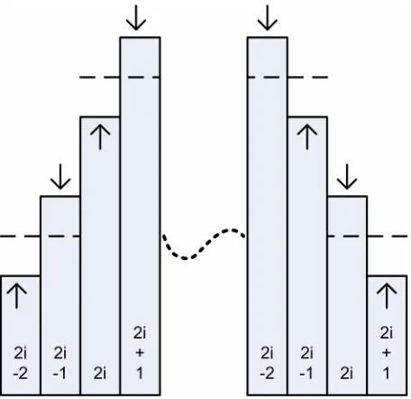
In order to explain the characteristics of b we can i classify different regions of a histogram into three classes of ascending, descending and flat regions. As shown in Fig. 1, the value of b increases for the i ascending and descending regions. For the flat regions of a histogram the value of b stays unchanged. i Therefore, the overall summation of b for the i histogram is an increasing value.
Another point is that the changes in α and β linearly dependent on the amount of the embedding. The reason is in the process of embedding data in the LSB of a cover image. A pseudo number generator by means of a specific key picks pixels of the image for the embedding purpose. This means a pixel is chosen only once. Therefore, the effect that a pixel has on the value of α and β is independent of the order that the pixel is chosen.
To explain the proposed steganalysis method two definitions, a theorem, and a lemma are stated in the followings:
Definition: The rate of change of α for 1 bit of
embedding in an image is R(α)
∑
= + − − = 127 0 i 1 2i 2i h h mn 1 )R(α where m and n are the image
side lengths.
Definition: The rate of change of α for 1 bit of
embedding in an image is R(α)
Definition: The rate of change of β for 1 bit of
embedding in an image is R(β)
Theorem: Σδ increases linearly as the embedding
increases.
Fig. 1 Increasing value of
i
b for ascending and descending regions.
Proof: Based on definition we know that
∑
= =127 0 i i i).p(a) R(a )R(α (9)
where a represents i h′2i,h′2i+1 and P(ai) is the probability of choosing a pixel for embedding purposes with either h′2ior h′2i+1 values. As shown in [19], this probability for a population of m×n is equal to
mn h
h′2i+ ′2i+1. Suppose that a pixel from bin i is picked,
then to find R(ai) without loss of generality we assume 1
2i 2i h
h < + . Hence we have:
(
)
(
)
(
) (
)
) 1 i 2 ( p ) i 2 ( p ) 2 / 1 ). 1 i 2 ( p 2 / 1 ). i 2 ( p ( 2 ) 0 ( p ). 1 i 2 ( p ) 1 ( p ). i 2 ( p 2 ) 0 , 1 i 2 ( p ) 1 , i 2 ( p 2 ) 1 i 2 value with pixel a in 0 Embedding ( p i 2 value with pixel a in 1 Embedding ( p 2 ) a ( R i + − = + − = + − = + − = + − = (10)In the Equation 10 notation p(2i,1) is the probability of embedding a 1 in a pixel with 2i value. Constant 2 is there because any change in the histogram would change ai by two units. In computation of Σδwe have 128 groups, where every two adjacent bins form a group. The number of pixels in the i th group is
1 2i 2i h
h + + , therefore the followings hold:
1 2i 2i 1 2i 1 2i 2i 2i h h h 1) p(2i , h h h p(2i) + + + + = + + =
Hence, we have:
0 h h h h h h h h h h ) R(a 1 2i 2i 1 2i 2i 1 2i 2i 1 2i 1 2i 2i 2i
i + <
− = + − + = + + + + +
Also, if we had h2i>h2i 1+ then:
0 h h h h h h h h h h ) R(a 1 2i 2i 2i 1 2i 1 2i 2i 2i 1 2i 2i 1 2i
i + <
− = + − + = + + + + +
Therefore, irrespective to the values of h and 2i h2i 1+
we have: 0 h h h h ) R(a 1 2i 2i 1 2i 2i
i + <
− − =
+ +
Now plugging R(ai)and P(ai) back into Equation 9 we have:
∑
∑
= = + + + + + = − − + − − =127 0 i 127 0 i 1 2i 2i 1 2i 2i 1 2i 2i 1 2i 2i h h mn 1 mn h h . h h h h ) R(αWe can also calculate the value of R(β) which turns out to be:
∑
= − + − −
− + − −
= 127
0 i
2 2k 1 2k 2k 1 2k 1 k
k n ).(h h h h )
sgn(n 2mn
1 R(β(
Since both R(α) and R(β) change linearly with embedding, their difference, Σδ , is a linear function of the amount of embedding.
Lemma: For an image without initial embedding α and
β are almost equal.
This is because that the distribution functions for images obtained from digital cameras or scanners cause the histograms to be almost piecewise linear which means
2i 1 2i 1 2i
2i h h h
h − − ≅ + − .
Considering the above mentioned definitions and lemma, to estimate the embedding rate (I) for an stego image using the image histogram, it is enough to first calculate the present value of sigma delta (Σδ ). Then I we should approximate the final value of sigma delta (Σδ100%). To get Σδ100% it is enough to replace all LSB's of image pixels with uniform random bits. We call this way of obtaining Σδ100% as simulation method. Another method to obtain Σδ100% is via Equations 4 to 8, which we refer to as analytical method. We see that the complexity of the analytical method, which uses the image histogram, is less than that of the simulation method, which works with all of the pixels of the image. It is expected that, when we increase embedding from zero to 100%, the plot starts at an initial point Σδ on I the vertical axis. Based on the mentioned theorem, the plot should linearly increase. The plot should also peak at a point, called Σδ100%, when 100% embedding is performed. The ratio of these two numbers, δ δ100%
I
∑ ∑
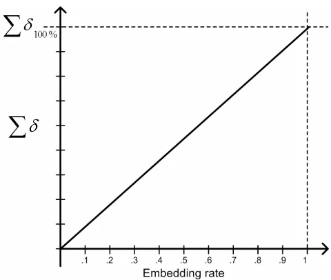
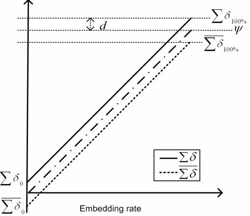
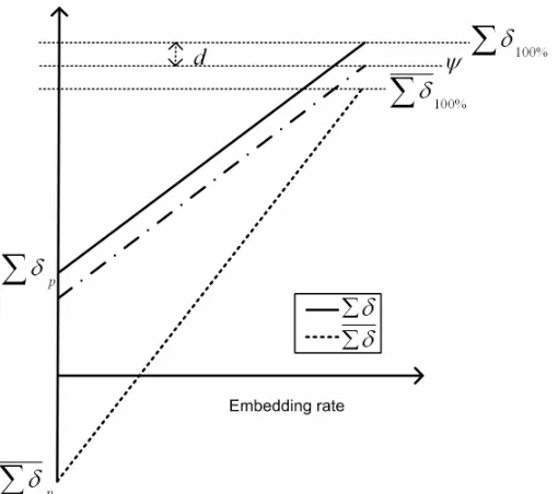
indicates the initial embedding rate.For an image with no initial embedding, Fig. 2 shows changes of the sigma delta value when replacing the LSB's of an image's pixels with random bits. Fig. 3 shows the changes that occur in the value of sigma delta for an image with some initial embedding (I). These graphs are formed incrementally. This means that after each bit of embedding the new value of sigma delta is plotted.
Adding 1 grayscale to all of the pixels of an image causes a switch between the values of α and β . Doing so may cause assignment of 256 to some pixels. We assign "0" to each of those pixels. It is equivalent to a circular shift of the histogram.
From now on we use Σδ′for an image with shifted histogram. For an image with no embedding the slope of Σδ and Σδ′ curves, obtained from the original histogram and its shifted version, are the same. Since the shifting of the histogram interchanges values of α and β , the initial value of δΣ ′ and Σδ curves at zero embedding have equal magnitudes and opposite signs,
I
I Σδ
δ
Σ ′=− . Therefore, when there is no embedding the δ
Σ ′curve is parallel to that of Σδ with a separation distance of 2ΣδI.
When all LSB's of an image's pixels are replaced with random bits, its Σδ diagram becomes horizontal. Further replacement of these LSB's with random bits would cause no further change in the diagram. This is due to the fact that paired bins of the histogram have reached binomial distribution and further embedding would cause no variation in the values of α and β . The value of the flat portion of the Σδ diagram is Σδ100% and that of Σδ′ is Σδ100%′ . The distance between Σδ′ and
100% δ
Σ ′ is independent of the amount of initial embedding. This distance is equal to the difference between Σδ and I Σδ′I when there is no embedding in the image.
Fig. 2 Sigma delta versus embedding rate for an image without initial embedding.
Fig. 3 Sigma delta versus embedding rate for an image with unknown (p) initial embedding.
Some singular points in the histogram where large number of very bright or very dark pixels exist cause the value of Σδ to be non-zero. Since 0 Σδ and I Σδ′I are symmetric, their midpoint occurs on zero. With these facts in mind and due to linearity of Σδ the amount of embedding can be calculated by the following relations:
m d δI p
2
) δ ( ) δ ( d
2
) δ ( ) δ ( ψ
100% 100%
100% 100%
− =
′ − =
′ + =
∑
∑
∑
∑
∑
(11)
The parameters that are used in Equation 11 are graphically presented in Figs. 4 and 5. The curves in
Fig. 4 show the situation where a hypothetical image under analysis has had no initial embedding. On the other hand the curves in Fig. 4 belong to an image where an unknown portion of the capacity has initially been used for embedding. The amount of embedding can be obtained by computing p in Equation 11.
The values of Σδ100% and Σδ100%′ that are used in Equation 11 can be computed from Equations 4 to 8 and they need not to be necessarily simulated. In another words Σδ100% can be obtained by calculating
∑
=
− 127
0 i
i i] E[A])
(E[B . In the same manner 100% δ
Σ ′ can be
computed by first shifting the histogram and then performing the same set of computations.
Fig. 4 Image under analysis with no initial embedding.
Fig. 5 Image under analysis with an unknown amount of initial embedding (I).
3 Simulation Results
In this section the results obtained from Σδ steganalysis method are presented. The simulator was written in C++ which performed the embedding in the LSBs of the pixels of images as well as performing the steganalysis. Two types of results are referred to in this paper. Analytical results are formed by taking an image and obtaining its histogram. Then using Equations 4 to 8 the values of Σδ100% and Σδ100%′ are predicted.
Subsequently, using Equation 11 the amount of embedding is calculated. On the other hand, the simulation results are formed by finding an image's histogram. Then 100 percent embedding is done and the values of Σδ100% and Σδ100%′ are directly obtained from the embedded image. Finally, using Equation 11 the amount of the initial embedded data is calculated. Fig. 6 shows Σδ diagram for a 1500×2100 pixel image obtained directly from a scanner. The image has had no initial embedding and was not subjected to any form of compression.
The horizontal axis of the plot in Fig. 6 is the percentage of LSB's replaced with random bits and the vertical axis represents Σδ and δΣ ′.
Now for the original mentioned image with no embedded data we see that the analytical results pronounce 1.28% embedding while the simulation results declare 1.24% initial embedding. This is one of many experimental results that show the functionality and accuracy of the suggested method.
Fig. 7 represents an example of another set of experiments where the image under analysis has initial embedding. In particular the image that was used in Fig. 7 had 50% initial embedding. The results from
computational procedure gave 47.6% initial embedding. The simulation results came up with 47.9% embedding in the image.
The following observations worth mentioning about Figs. 6 and 7:
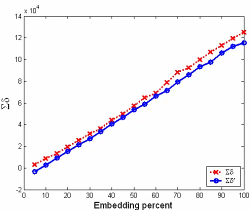
1-The Σδ curve in Fig. 7 starts at a point on the vertical axis which is half way between the maximum value of the curve at 100% embedding. This means that the image has had fifty percent initial embedding.
2-The initial values of Σδ and δΣ ′ curves are perfectly symmetric in both Figs. 6 and 7.
3-The slop of the Σδ′ curve in the image with 50% initial embedding is more than the corresponding curve in the same image with zero initial embedding. While the ultimate values of these curves are equal, the initial value of δΣ ′ curve is much lower for the image with embedded data.
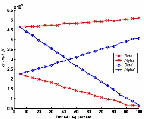
For a shifted histogram the values mentioned in Equation 3 are presented by α′ and β′. In Figs. 8 and 9 parameters α , β , α′ and β′ are plotted. The initial values of α and β′ as well as the initial values of β and α′ are equal. These plots support the claims that Σδ curve is a linear and ascending function. It can be seen that α and α′ are descending functions while β and β′ are ascending and therefore, β−α=∑δ would be an ascending function.
Fig. 6 Σδ curves for an image with zero initial embedding.
Fig. 7 Σδ curves for an image with 50% initial embedding.
Fig. 8 α, β, α′ and β′parameters for an image with no initial embedding.
Fig. 9 α, β, α′ and β′parameters for an image with 50% initial embedding.
The proposed method showed high precision for scanned images. The obtained results for images that were initially compressed by JPEG were highly precise. In one experiment some 35 scanned images were subjected to different levels of embedding. The Σδ algorithm found the amount of embedding with an average error of -0.0021 and with standard deviation of error being 0.048.
In another experiment, 40 images were scanned using an HP Scanjet 3800. Each image was infected 50 times with random embedding rates. These 2000 samples were analyzed using analytical sigma delta and simulation based sigma delta. The mean and variance of errors for these experiments were computed. The mean and average of error for the simulation based sigma delta was computed 0.052 and 0.0152 respectively. Using the analytical sigma delta, the mean and variance of errors were computed as 0.0025 and 0.0037 respectively. The analytical results are much more accurate than the results from the simulation based sigma delta.
Same set of samples were analyzed using the RS steganalysis. The mean and variance of the errors were calculated as 0.0070 and 0.0182. The results from RS are better than the results from the simulation based sigma delta. On the other hand, the analytical based sigma delta performs better than the RS steganalysis. In another set of experiments 160 JPEG photographs with various textures were taken by a Sony DSC-F828 Camera, were used. Each of these images was infected 30 times with random embedding rate. These 4800 samples were analyzed using the simulation, the analytical based sigma delta, and the RS steganalysis. The mean and variance of the errors were calculated. For the simulation based sigma delta, the computed mean and variance were 0.0616 and 0.0121 respectively. For the analytical sigma delta these values were 0.0039 and 0.0066. For RS these values were 0.0050 and 0.0015 which are slightly better than the results from the analytical sigma delta.
Summery of these experiments is shown in Table 1.
Table 1: Comparison of Sigma delta with RS.
Mean Variance
Σδ Σδ
Image Source Number of
samples RS
Simulation Analytical
RS
Simulation Analytical
Scanner:
(HP Scanjet 3800) 2000 0.007 0.052 0.0025 0.018 0.0152 0.0037
Camera:
(Sony DSC-F828) 4800 0.005 0.0616 0.0039 0.0015 0.0121 0.0066
4 Conclusions
In this paper a new steganalysis method called Σδ was introduced. The suggested method is able to detect the
amount of embedded data that exist in the LSB of pixels of an image using LSB replacement method. The behavior of the histogram of an image is the basis of the
proposed method. By just obtaining the histogram of an image, through mathematical analysis the size of embedded information can be calculated. Raw scanned images and JPEG filtered images were used to show that both mathematical analysis as well as simulation can extract the size of the embedded data. In all cases the simulation outcomes verified the analytical results. The proposed method compared to the one introduced in [10] by Fridrich is less complex. The RS method needs twice to compute regular and singular groups and also needs a flipping operation performed on all of the pixels. Therefore, the RS attack has higher computational complexity than the Σδ steganalysis while the accuracies of both methods are compatible. In using sigma delta, it is enough to extract an image histogram and apply Equations 4 to 8, in order to calculate the initial value of embedding.
References
[1] Dumitrescu S., Wu X. and Wang X., “Detection of LSB steganography via sample pair analysis,” IEEE Transactions on Signal Processing, Vol. 51, No. 7, pp. 1995-2007, 2003.
[2] Hopper N., Toward a theory of steganography, Ph.D. Thesis, School of Computer Science, Carnegie Mellon University, July 2004.
[3] Westfeld A., “F5 A steganographic algorithm: High capacity despite better steganalysis,” Proceedings of 4th International Information Hiding Workshop, Springer-Verlag, Vol. 2137, pp. 289-302, 2001.
[4] Swanson M., Kobayashi M., and Tewfik A., “Multimedia data embedding and watermarking technologies,” Proceedings of the IEEE, Vol. 86, No. 6, pp. 1064-1087, 1998.
[5] Cox I., Kilian J., Leighton T. and Shamoon T., “Secure spread spectrum watermarking for multimedia,” IEEE Transactions on Image Processing, Vol. 6, No. 12, pp. 1673-1687, 1997. [6] Provos N., “Defending against statistical
steganalysis,” Proceedings of 10th Usenix Security Symposium, pp. 323-335, 2001.
[7] Fridrich J., Goljan M., and Du R., “Steganalysis based on JPEG compatibility,” Proceedings of Special Digital Watermarking Data Hiding, pp. 275-280, 2001.
[8] Fridrich J., Du R. and Meng L., “Steganalysis of LSB encoding in color images,” Proceedings of IEEE International Conference on Multimedia, Vol. 3, pp. 1279-1282, 2000.
[9] Westfeld A. and Pfitzman A., “Attacks on steganographic systems,” Proceedings of 3rd International Information Hiding Workshop, Springer-Verlag, pp. 61-76, 1999.
[10] Fridrich J., Goljan M. and Du R., “Reliable detection of LSB steganography in grayscale and color image,” Proceedings of ACM: Special
Session on Multimedia Security and Watermarking, pp. 27-30, 2001.
[11] Celik M., Sharma G. and Tekalp A. M., “Universal image steganalysis using rate-distortion curves,” Proceedings of SPIE: Security and Watermarking of Multimedia Contents VI, Vol. 5306, pp. 467-476, 2004.
[12] Ker A., “Quantitative evaluation of pairs and RS steganalysis,” Proceedings of SPIE: Security, Steganography, and Watermarking of Multimedia Contents VI, Vol. 5306, pp. 83-97, 2004.
[13] Zhang T. and Ping X., “A new approach to reliable detection of LSB steganography in natural images,” Elsevier Journal of Signal Processing, Vol. 83, pp. 2085–2093, 2003. [14] Bohme R. and Ker A., “A two factor-model for
quantitative steganalysis,” Proceedings of SPIE: Security, Steganography, and Watermarking of Multimedia Contents VIII, Vol. 6072, pp. 59-74, 2006.
[15] Mahdavi M., Samavi S., Zaker N. and Mansori F., “A new steganalysis method for LSB flipping steganography based on local gradient of image histogram,” 12th international computer conference, pp. 170-178, 2007.
[16] Hasheminejad M., Ashrafi M. and Toufighi S., “A new method to reveal hidden data in images,” (Persian), 4th Iranian society of cryptography conference, pp. 151-158, 2007.
[17] Fridrich J. and Goljan M., “Practical steganalysis of digital images-state of the art,” Proceedings of SPIE: Security and Watermarking of Multimedia Contents IV, Vol. 4675, pp. 1-13, 2002.
[18] Prem S. and Puri S., “Probability generating functions of absolute difference of two random variables,” Proceedings of the National Academy of Sciences of the United States of America, Vol. 56, No. 4, pp. 1059-1061, 1966.
[19] Ross S. M., Stochastic processes, John Wiley and Sons, 1996.
Mojtaba Mahdavi received his
B.Sc. degree in Computer
Engineering in 1999, and his M.Sc. degree in Computer Architecture in 2002, both from the Electrical and Computer Engineering department of Isfahan University of Technology (IUT), Isfahan, Iran. From Autumn of 2004 he has been a Ph.D. candidate in the field of Computer Engineering at the ECE department of IUT. Mr. Mahdavi’s main research area is in the field of data hiding and steganography.
Shadrokh Samavi is a professor of
Computer Engineering at the
Electrical and Computer
Engineering Department, Isfahan University of Technology, Iran. He completed a B.Sc. degree in Industrial Technology (1980) and received a B.Sc. degree in Electrical Engineering (1982) at California State University, a M.Sc. degree (1985) in Computer Engineering at the University of Memphis and a Ph.D. degree (1989) in Electrical Engineering at Mississippi State University, U.S.A. Professor Samavi's research interests are in the areas of image processing and hardware implementation and optimization of image processing algorithms. He is also interested in watermarking and related subjects. Dr. Samavi is a Registered Professional Engineer (PE), USA. He is also a member of IEEE and a member of Eta Kappa Nu and Tau Beta Pi honor societies.
Nazanin Zaker was born in Isfahan,
Iran. She received her B.Sc. degree
from Isfahan university of
Technology in 2007 in the field of Computer Engineering. She is a
master student in Software
Engineering at Shiraz University. She is now conducting research on semantic webs and its aspects in software engineering. Her research interests are semantic webs and web services, different aspects of software engineering, data hiding and specifically steganography in the spatial domain of bitmap images, and computer security.
Mahmoud Modarres-Hashemi
received his B.Sc. and M.Sc. degrees in electrical engineering in 1990 and 1992 from the Electrical
and Computer Engineering
department of Isfahan University of Technology (IUT), Isfahan, Iran. He
pursued his studies at the
department of Electrical
Engineering of Sharif University of Technology, Tehran, Iran, where he received his Ph.D. in 2000. Dr. Modarres-Hashemi is currently an assistant professor at the ECE department of IUT. His research interests are Detection Theory, Radar Signal Processing, Electronic Warfare, Cryptography, and Channel Coding.