A b s t r a c t. This study was planned to examine the use of LandSat ETM+images to develop a model for monitoring spatial variability of soil cation exchange capacity in a semi-arid area of Neyshaboor. 300 field data were collected from specific GPS re-gistered points, 277 of which were error free, to be analysed in the soil laboratory. The statistical analysis showed that there was a small R-Squared value, 0.17, when we used the whole data set. Visual interpretation of the graphs showed a trend among some of the data in the data set. Forty points were filtered based on the trends, and the statistical analysis was repeated for those data. It was discove-red that the 40 series were more or less in the same environmental conditions; most of them were located in disturbed soils or aban-doned lands with sparse vegetation cover. The soil was classified into high and medium salinity, with variable carbon (1.0 to 1.6%), heavy textured and with high silt and clay. Finally it was concluded that two different models could be fitted in the data based on their spatial dependency. The current models are able to explain spatial variability in almost 45 to 65% of the cases.
K e y w o r d s: soil cation exchange capacity, remote sensing, soil properties, soil spatial variability
INTRODUCTION
Using remote sensing technology often reduces costs and increases accuracy and speed. By using remote sensing data three main categories of information are recognised: soil properties based on its reflectance band and the resulting images, the effect of soil surface conditions on the reflected radiation, and the simulated patterns which can be used for producing maps of soil variability (Johannsenet al., 1998).
The most comprehensive and detailed geographical world soil resources are presented in the global soil map in the scale of 1:5 000 000. This map is an integrated national and regional map based on a common legend. It contains different information including available water capacity,
soil organic carbon content, soil pH, soils cation exchange capacity (CEC), soil drainage classes, soil depth classes and so on. The density and quality of available profiles is drama-tically variable from one area to another (Batjes, 2002).
Different studies show that the relationship between satellite data and soil characteristics is more clear in 3.0 to 8.2mm. Spectral response in this band is due to differences in organic matter content, iron levels, soil moisture and soil texture. The highest correlation with soil characteristics derived from the reflected bands data is known as albedo (Postet al., 2000).
In the saline area, most of the signal strengths are related to soluble salt concentration, while in non-saline soil, EC variability of soil is a function of organic matter content, soil texture, soil moisture and soil cation exchange capacity (Barneset al., 2003).
Matinfaret al. (2011) used ASTER sensor data in order to study soils, and their results showed soils which have soft and dark uneven surfaces that are well separated in visible and thermal wave.
Fox and Metla (2005) took three types of soil line and used PCA (Principal component analysis) and regression analysis to assess soil characteristics, including soil organic carbon and exchange capacity. Those were compared and showed that PCA with high correlation (R2= 0.32) gave bet-ter results for describing soil characbet-teristics changes than the other two analysis methods. The researchers suggested that PCA could be used as a method of sampling in determining location of soil samples compared to the soil line model.
Remote sensing technology has a high potential for the characterisation of the spatial variation of soil properties at large scales, so this approach can provide valuable information for application to precision agriculture and environmental Int. Agrophys., 2013, 27, 409-417
doi: 10.2478/intag-2013-0011
Using satellite data for soil cation exchange capacity studies
M. Ghaemi
1, A.R. Astaraei
1, S.H. Sanaeinejad
2, and H. Zare
31Department of Soil Science,2Department of Water Engineering,3Department of Agronomy, Ferdowsi University of Mashhad, FUM Campus, Azadi Sq., Mashhad, Khorasan Razavi, Iran
Received July 31, 2012; accepted October 29, 2012
© 2013 Institute of Agrophysics, Polish Academy of Sciences
*Corresponding author e-mail: [email protected]
pacity in soil was also investigated. MATERIAL AND METHODS
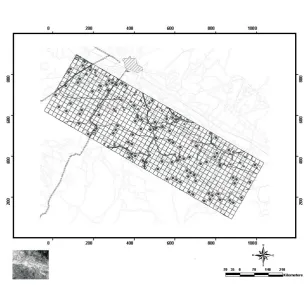
The study area was located in the Neyshaboor plain in Khorasan-Razavi province in the N-E of Iran, geographi-cally located between longitudes 58.57 to 59.13° and lati-tudes 35.85 to 36.25° (Fig. 1). The climate is arid to semi-arid, with annual average temperature of 14.5°C and preci-pitation of 250 mm based on Ambergeh climate classifi-cation method. According to land-use maps, this area is ge-nerally saline with agricultural activities.
LandSat ETM+images including 6 bands with 30 m re-solution, one thermal band with 60 m resolution and a pan-chromatic band with 15 m resolution, from track 160 and row 35, taken on 10th of July 2002, were used. The images were originally corrected for general geometric and radiometric errors.
However, more geometric corrections were also applied for more confidence. Various image processing techniques were used, including image enhancement, PCA, tasseled cap transformation, and also 50 vegetation and soil indices derived from the images. Some of the indices are listed in Table 1.
The ETM+images were converted into an appropriate format to be used in ERDAS Imagine 8.6 and IDRISI Kilimanjaro software.
After pre-processing of the images, their general fea-tures were compared with the corresponding land use map (scale: 1:250 000). A part of Neyshaboor plain with 765 km2 was selected based on soil properties and vegetation cover estimated from field observations. That area is contained in an area of 1 881×1 497 pixels in the image. The area was divided into three main parts depending on their salinity determined from land use map and field observations. A grid with 10×50 mesh was drawn, with 1 000 m grid length on the area (Fig. 2). 100 of the grid cells were randomly selected and 3 separate points 100 m apart were chosen in each se-lected cell as sampling points. A sample of soil (20×20 cm surface and 20 cm depth) was recovered from each sampling point. The geographic position was recorded by a Garmin GPS and the samples were transported to a soil laboratory for testing.
The recovered soil samples were air dried and then sieved through a 2 mm sieve for laboratory testing. Different parameters were measured, including soil acidity by using a pH meter, EC in soil saturation extracts by an EC meter,
cation exchange capacity values and the values of spectral satellite image were evaluated. Then the most appropriate independent variables were selected to estimate the de-pendent variables based on a multivariate linear regression (stepwise regression) equation. All the coefficients were con-sidered statistically significant at 95% confidence level.
RESULTS AND DISCUSSION
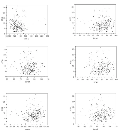
The R-Square was low when all of the data from the low to high salinity soil samples were considered in the regres-sion analysis (Table 2). The highest R-squares were obtain-ed between the main bands, including bands 1, 2 and 3, the amounts for which were 0.06 0.04 and 0.1, respectively. Indices (PD311 = TM3-TM2), (PD321 =TM3-TM1), BI1, SI showed a higher correlation. Appropriate model for achiev-ing stepwise regression method was applied and the va-riables with the highest R-square were used to obtain Eq. (1) for the total data set.
Fig. 1.Geographical location of the study area.
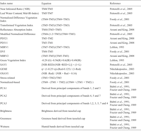
Index name Equation Reference
Near Inferared Ratio ( NIR) TM4/TM3 Pettorelliet al., 2005
Leaf Water Content( Mid-IR-Index) TM5/TM7 Pettorelliet al., 2005
Normalized Difference Vegetation
Index (TM4-TM3)/(TM4+TM3) Foodyet al., 2001
Transformed Vegetation Index (TM5-TM3)/(TM5+TM3) Pettorelliet al., 2005
Reflectance Absorption Index TM4/(TM3+TM5) Arzani and King, 2008
Modified Normalized Difference (TM4-(1.2×TM3)/(TM4+TM3) Pettorelliet al., 2005
PD321 TM3-TM2 Arzani and King, 2008
PD311 TM3-TM1 Arzani and King, 2008
MIRV1 (TM7-TM3)/(TM7+TM3) Leblon, 1993
DVI TM4-TM3 Foodyet al., 2001
MIRV2 (TM5-TM3)/(TM5-TM3) Arzani and King, 2008
Green Vegetation Index -0.29 (G) -0.56(R)+0.6(IR)+0.49(IR) Leblon, 1993
SAVI [NIR-RED)/(NIR+RED+L)] × (1+L) Pettorelliet al., 2005
GEMI h× (1-0.25×h)-(Red-0.125) / (1-Red) Nikolakopoulos , 2003
OSAVI (NIR -Red) / (NIR + Red + 0.16) Nikolakopoulos , 2003
Stress-related (TM1×TM2)/TM3 Foodyet al., 2001
Normalized-based (TM4 - (TM1 + TM2) )/(TM4 + (TM1 + TM2) ) Foodyet al., 2001 PCA1 Derived from principal components of bands 1, 2 and 3 Bahttiet al., 1991;
Frazier and Cheng, 1989 PCA2 Derived from principal components of bands 4, 5 and 7 Bahttiet al., 1991;
Frazier and Cheng, 1989 PCA3 Derived from principal components of bands 1,2, 3, 5, 7 and 4 Bahttiet al., 1991;
Frazier and Cheng, 1989
Brightness Brightness derived from tasseled cap Bahttiet al., 1991;
Frazier and Cheng, 1989 Greenness Greeness band derived from tasseled cap Bahttiet al., 1991;
Frazier and Cheng, 1989 Wetness Humid bands derived from tasseled cap BahttiFrazier and Cheng, 1989et al., 1991;
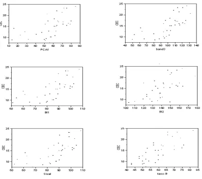
The results showed that the 40 series were located in degraded and abandoned agricultural lands with scattered vegetation cover. The areas contain moderate to high sali-nity lands in the area. Organic carbon in these parts is va-riable between 1 and 1.6%. Total amounts of silt and clay in these lands are high and heavy textured soils are included (Fig. 5). This shows that high levels of organic carbon in the low density vegetation areas (due to destruction of vegeta-tion) are affected by the amount of cation exchange capacity and percentage of clay, especially high electrical conduc-tivity, in the region which is similar to the results reported by Vagenet al. (2006). Field observations also showed that wa-ter level in those points is high. On the other hand, the effects of salt and sodium on the soil surface were also observed.
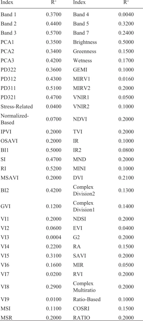
Because of all subscription and spectral characteristics of physical and chemical soil in these parts, another regression analysis was performed. The R-square for the remaining points were re-calculated and it was found that higher R-square values were obtained in relation to the general state when all of the data were considered. For example, R-square was 0.1 for band 3 for the whole data set while it was increased to 0.36 and 0.57 for the rest of the data set and the 40 series, respectively (Tables 3 and 4).
Therefore, the R-square value, which is statistically significant at the 5% level, is high only when the cation exchange capacity and digital values from combination bands are used. The highest R-square was derived for the 40 series when the original bands 1, 2, 3, the indices and the
analysis of RI, SI, BI1, BI2, PD311, PD321, PCA3 and brightness components were applied. The highest R-square for the rest of points was derived when band 3, the indices and the analysis of PCA1, PD321, GEMI, VI5, BI1 and SI were applied in the regression equation.
The results showed that principal component analysis and regression models can be used to assess soil properties in-cluding cation exchange capacity. Fox and Metla (2005) also obtained similar results in Mid-West of the United States. For the separated homogeneous data the regression coefficients increased considerably. R-square = 0.65 was ob-tained when the 40 series was applied, which shows a good correlation and dependency between the values. After sepa-rating the data series, it was observed that the residual data also showed higher R-square value. Figure 6 shows the scatter diagrams of cation exchange capacity obtained by the models for the 40 series and the rest of the data set.
As it can be seen in Fig. 7, most of the data values are located in the range of 95%. Band 3 and PD311 were used for series 1 and band 3 and PD321 were used for series 2 to estimate cation exchange in the study area. These data provide higher R-square and lower RMSE when the data applied in the regression analysis are taken from the area with homogenous characteristics. In this analysis it was found that after fitting the data Eq. (2) (R-square = 0.62 and RMSE = 2.87) and Eq. (3) (R-square = 0.47 and RMSE = 2.13) for series 1 and 2, respectively can be considered as appro-priate models for estimating this variable.
Index R2 Index R2
Band 1 0.06000 Band 4 0.00300
Band 2 0.04000 Band 5 0.00800
Band 3 0.10000 Band 7 0.01000
PCA1 0.01000 Brightness 0.00200
PCA2 0.00800 Greenness 0.00050
PCA3 0.00300 Wetness 0.00006
PD322 0.04000 GEMI 0.00040
PD312 0.01000 MIRV1 0.00001
PD311 0.02700 MIRV2 0.00002
PD321 0.05000 VNIR1 0.00030
Stress-Related 0.00040 VNIR2 0.00050
Normalized-Based 0.00070 NDVI 0.00100
IPVI 0.00200 TVI 0.00100
OSAVI 0.00300 IR 0.00050
BI1 0.00800 IR2 0.00070
SI 0.00300 MND 0.00010
RI 0.00260 MINI 0.00070
MSAVI 0.00300 DVI 0.00020
BI2 0.00520 Complex
Division2 0.00070
GVI 0.00080 Complex
Division1 0.00030
VI1 0.00100 NDSI 0.00100
VI2 0.00003 EVI 0.00200
VI3 0.01000 G2 0.00040
VI4 0.00016 RA 0.00020
VI5 0.00230 SAVI 0.00200
VI6 0.00180 MIR 0.00022
VI7 0.00001 RVI 0.00001
VI8 0.00002 Complex
Multiratio 0.00200
VI9 0.00002 Ratio-Based 0.00100
MSI 0.00040 COSRI 0.00100
MSR 0.00100 RATIO 0.00080
T a b l e 2 .R-squares derived from regression between different
vegetation indices and CEC applying the total data
Index R2 Index R2
Band 1 0.2500 Band 4 0.0700
Band 2 0.2200 Band 5 0.1600
Band 3 0.3600 Band 7 0.1800
PCA1 0.3000 Brightness 0.2000
PCA2 0.2000 Greenness 0.2000
PCA3 0.2300 Wetness 0.1100
PD322 0.2000 GEMI 0.2600
PD312 0.1100 MIRV1 0.0200
PD311 0.2000 MIRV2 0.0400
PD321 0.3300 VNIR1 0.0300
Stress-Related 0.0400 VNIR2 0.0500
Normalized-Based 0.0700 NDVI 0.1000
IPVI 0.2000 TVI 0.1000
OSAVI 0.2000 IR 0.0500
BI1 0.2800 IR2 0.0700
SI 0.3000 MND 0.0100
RI 0.2400 MINI 0.0700
MSAVI 0.2000 DVI 0.0200
BI2 0.2500 Complex
Division2 0.0800
GVI 0.0800 Complex
Division1 0.0200
VI1 0.1000 NDSI 0.1000
VI2 0.0004 EVI 0.0200
VI3 0.0400 G2 0.1600
VI4 0.0100 RA 0.0200
VI5 0.2300 SAVI 0.2000
VI6 0.1400 MIR 0.1000
VI7 0.0100 RVI 0.1600
VI8 0.0200 Complex
Multiratio 0.0400
VI9 0.0200 Ratio-Based 0.2000
MSI 0.0400 COSRI 0.1000
MSR 0.1000 RATIO 0.1000
T a b l e 3.R-squares derived from regression between different
CEC= -8.05+0.37 PD321+0.13 b3 (2) CEC= 9.15 +0.24 PD311+0.15 b3 (3) Statistical analysis showed that PD321 and PD311 in-dices are more correlated with the amount of cation exchan-ge capacity than other bands. It should be noted that band 1, 2 and 3 are involved in calculating both of the indices.
Therefore, experimental data with homogeneous cha-racteristics have more effects on reflectance, so that the effect could be seen as a similar trend in all of the image processing used for monitoring of the changes in the region.
The above results are similar with the ones that Huete (1996) reported. This shows that the digital analysis of ETM+images can be used for evaluation of natural pheno-mena and land cover.
The results of spectral analysis showed that the total values of silt and clay in the segregated parts of the study area is high, which affected soil darkness and therefore resulted in more light absorption. Research in this field by Whiteet al. (1997) showed that soils with high amounts of sand have almost no absorption in the visible and infrared band. Formaggio et al. (1996) also reported that the re-sulting reflectance bands from soils with higher CEC are much lower than other soils.
0 5
90 100 120 140 160 180 200 220 240 tass-G
0 5
10 20 30 40 50 60 70 80 90 100 PCA1
0 5 10 15 20 25
CE
C
50 60 70 80 90 100 110 band1
0 5 10 15 20 25
CE
C
30 40 50 60 70 80 90 100 110 PCA2
0 5 10 15 20 25
CE
C
40 50 60 70 80 90 100 110 120 130 140 150 band3
0 5 10 15 20 25
CE
C
50 60 70 80 90 100 110 band2
CONCLUSIONS
1. Accordingly, the potential of remote sensing for soil variability in arid and semi-arid areas is limited because of special features of land cover and soils in those areas.
2. Using different image processing such as band ratios and principal component analysis increased R-squared values and provided better information than single band analysis. However, care must be taken in selecting appro-priate methods according to the area features and the highest correlation coefficient.
3. The analysis of digital numbers showed that ETM+ images have a great potential for the evaluation of soil properties in areas with homogenous features.
4. The practical results can be used for applying proper management programs in the study area. It was also conclu-ded that because of complexity in soil properties radiation signature it is hard to distinguish different soil properties by using only remote sensing data. Finally, this study showed that spatial analysis is essential for the study area because the soil properties are varied spatially very much.
(b
)
(a
)
(d
)
(c
)
Fig. 4.Scatter diagram soil cation exchange capacity against digital numbers in some of the analyses (the 40 series was used).
Fig. 5. Geographical positions of the 40 series data points with
40 50 60 70 80 90 100 110 120 130 140 band3 10 15 20 25 CE C
-10 0 10 20 30 40 50 60 PD311 10 15 20 25 CE C A ct u a l
10 15 20 25
CEC Predicted P<.0001 RSq=0.65 RMSE=2.8768
Fig. 6.Scatter diagram of soil cation exchange capacity against the
image digital numbers when the 40 series data were applied.
1 3 5 7 9 11 13 15 CE C
80 90 100 110 120 130 140 band3 1 3 5 7 9 11 13 15 CE C
15 20 25 30 35 40 45 PD321 1 3 5 7 9 11 13 15 C E C A ct u al
1 2 3 4 5 6 7 8 9 10 11 12 13 14 15 CEC Predicted P<.0001 RSq=0.47 RMSE=2.1351
Fig. 7.Scatter diagram of soil cation exchange capacity against the
image digital numbers when the remaining data were applied excluding the 40 series data.
Band 2 0.4400 Band 5 0.3200
Band 3 0.5700 Band 7 0.2400
PCA1 0.3500 Brightness 0.5000
PCA2 0.3400 Greenness 0.1500
PCA3 0.4200 Wetness 0.1700
PD322 0.3600 GEMI 0.1000
PD312 0.4300 MIRV1 0.0160
PD311 0.5100 MIRV2 0.2000
PD321 0.4700 VNIR1 0.0500
Stress-Related 0.0400 VNIR2 0.1000
Normalized-Based 0.0700 NDVI 0.2000
IPVI 0.2000 TVI 0.2000
OSAVI 0.2000 IR 0.1000
BI1 0.5000 IR2 0.0800
SI 0.4700 MND 0.2000
RI 0.5200 MINI 0.1000
MSAVI 0.2000 DVI 0.2100
BI2 0.4200 Complex
Division2 0.1300
GVI 0.1200 Complex
Division1 0.1400
VI1 0.2000 NDSI 0.2000
VI2 0.0600 EVI 0.0400
VI3 0.0004 G2 0.2000
VI4 0.2200 RA 0.1500
VI5 0.3100 SAVI 0.2000
VI6 0.1600 MIR 0.0500
VI7 0.0200 RVI 0.2000
VI8 0.2900 Complex
Multiratio 0.2000
VI9 0.0100 Ratio-Based 0.1000
MSI 0.1100 COSRI 0.1500
REFERENCES
Arzani H. and King G.W., 2008.Application of remote sensing
(landsat TM data) for vegetation parameters measurement in western division of NSW. Int. Grassland Congr., 29 June – 5 July, Hohhot, China.
Bahtti A.U., Mulla D.J., and Frazier B.E., 1991.Estimation of
soil properties and wheat yields on complex eroded hills using geostatistics and thematic mapper images. Remote sens. Environment, 31, 181-191.
Barnes E.M., Sudduth K.A., Hummel J.W., Lesch S.M., Corwin
D.L., Yang C., Daughtry C.S.T., and Bausch W.C., 2003.
Remote and ground-based sensore techniques to map soil properties. Photogrammetric Eng. Remote Sensing, 69(6), 619-630.
Batjes N.H., 2002. isric-wise global data set of derived soil
properties on a 0.5 by degree grid (version 2). international soil reference and information center (ISRIC). Report, 2003/03 http:.\\www.isric.org), wageningen, 1-14
Chapman H.D., 1965.Cation exchange capacity. In: Black, C.A.
etal. (eds.). Methods of Soil Analysis: Part 2. Monograph, Am. Soc. Agronomy, 9, 891-901.
Dematte J.A.M., Galodos M.V., Guimaraes R.V., Genu A.M.,
Nanins M.R., and Zullo J., 2007.Quantification of tropical
soil attributes from ETM+ LANDSAT-7 data. Int. J. Remote Sensing, 17(28), 3813-3829.
Foody G.M., Cutler M., Mcmorrow J., Pelz D., Tangki H.,
Boyd D.S., and Douglas I., 2001.Mapping the biomass of
Bornean tropical rain forest from remotely sensed data. J. Global Ecology Biogeography, 10, 379-387.
Formaggio A.R., Epiphanio J.C.N., Valeriano M.M., and
Olivera J.B., 1996.Comportamento spectral (450-2.450 nm)
de solos tropic is de Sao Paulo [Spectral (450-2450 nm) behavior of tropical soils from the State of Sao Paulo]. Revista Brasileira de Ciencia do Solo, 20, 467-474.
Fox G.A. and Metla R., 2005.Soil property analysis using
prin-cipal components analysis, soil line and regression models. J. Soil Sci. Soc. Am., 69, 4782-1788.
Frazier B.E. and Cheng Y., 1989.Remote sensing of soils in
eastern palouse region with landsat thematic mapper, Remote sense. Environment, 28, 317-325.
Gee G.W. and Bauder J.W., 1986.Particle-size analysis. In:
Methods of Soil Analysis Part 1. Soil Science Society of America Book Series 5, Madison, WI, USA.
Huete A.R., 1996. Extension of soil spectra to the satellite:
atmosphere, geometric and sensor considerations. Photo-interpretation, 34, 101-114.
Johannsen C.J., Carter P.G., Willis P.R., Owubah E., Erickson B.,
Ross K., and Targulian N., 1998.Applying remote sensing
technology to precision farming. Proc. IV Int. Conf. Pre-cision Agriculture, July 19-22, St. Paul, MN, USA.
Leblon B., 1993. Soil and vegetation optical properties. In:
Applications in Remote Sensing, Volume 4, The Inter-national Center for Remote Sensing Education. Wiley Press, New York, USA.
Matinfar H.R., Sarmadian F., and Alavipanah S.K., 2011.Use
of DEM and ASTER sensor data for soil and agricultural characterizing. Int. Agrophys., 25, 37-46.
Nikolakopoulos K.G., 2003. Use of vegetation indexes with
ASTER VNIR data for burnt areas detection in Western Peloponnese, Greece. IEEE Int. Geoscience and Remote Sensing Symp., September 21-25, Toulouse, France.
Pettorelli N., Vik J.O., Mysterud A., Gaillard J.M., Tucker C.J.,
and Stenseth N.C., 2005.Using the satellite-derived NDVI
to assess ecological responses to environmental change. J. Trends Ecology Evolution, 9(20), 503-510.
Phillips J.D., 1994.Deterministic uncertainty in landscapes Earth
Surface proc. Landforms,19, 389-401.
Post D.F., Fimbres A., Matthiass A.D., Sano E.E., Accioly L.,
Batchily A.K., and Ferreira L.G., 2000.Predicting soil
albedo from soil color and spectral reflectance data. Soil Sci. Soc. Am. J., 64(3), 1027-1034.
Vagen T.G., Shepherd K.D., and Walsh M.G., 2006.Sensing
landscape level change in soil fertility following de-forestation and conversion in the highlands of Madagascar using Vis-NIR spectroscopy. Geoderma, 133, 281-294.
Walkely A. and Black I.A., 1934. An examination of the
Degtjareff method for determining soil organic matter and a proposed modification of the chromic acid titration method. Soil Sci., 37, 29-38.
White K., Walden J., Drake N., Eckardt F., and Settle J., 1997.