A Computational Meshless Method for Solving
Multivariable Integral Equations
E. Babolian
1,*and F. Fattahzadeh
21
Department of Mathematics, Teacher Training University, Tehran, Islamic Republic of Iran
2
Department of Mathematics, Islamic Azad University, Research and Science Campus Tehran, Islamic Republic of Iran
Abstract
In this paper we use radial basis functions to solve multivariable integral
equations. We use collocation method for implementation. Numerical experiments
show the accuracy of the method.
Keywords: Multivariable integral equation; Meshless method; Radial basis functions
*
Corresponding author, Tel.: +98(21)44094051, Fax: +98(21)77602988, E-mail: [email protected]
1. Introduction
In many literatures univariable integral equations have been solved with projection methods as Collocation and Galerkin methods and with different types of basis functions such as wavelets or other (orthogonal) basis functions [1-9]. In some projection methods such as Collocation one can use interpolation scheme; but as we know in the case of two or more variables case there is not any natural generalization of interpolation [10-13]. Other methods such as finite element which uses (orthogonal) basis functions actually needs mesh generation for domain of integration. Mesh dependent methods need some triangulation (or rectangulation) and coding for nodes of each triangle (or rectangle) therefore some introductive algorithms should be executed before implementation of the underlying method [2]. Here we solve multivariable I.E. with some meshless methods.
To simplify the notation we consider only functions of two variables. Generalizations of functions in more than two variables should be fairly straightforward.
2. Multivariable I.E. and Radial Basis Functions
Consider the following I.E. of the first and second
kind with two variables
(
) (
)
(
)
(
)
[ ] [ ]
, , , , ,
, , ,
y x
c a k x y d x y
x y a b c d
ξ η ρ ξ η ξη ψ=
∈ ×
∫ ∫
(1)
(
)
(
) (
)
(
)
(
)
, , , , ,
, , ,
R
x y k x y d d
x y x y R
λρ ξ η ρ ξ η ξ η
ψ
−
= ∈
∫
(2)
where R, is a bounded region in the plane \2. In this section we apply projection methods to the above equation without needing any triangulation of R.
2.1. Scattered Data Interpolation
Given a region R in plane \2, and a set of data
(measurement, and locations at which these measurements were obtained) we want to find a rule which exactly match the given measurements at the corresponding locations. If the locations at which the measurements are taken are not on a uniform or regular grid then the process is called Scattered data interpolation.
f
P is a linear combination of certain basis functions
k
B , i.e.,
( )
( )
,N
s k k
f X =
∑
c B X X ∈\P (3)
Here we use scattered data interpolation to find the solution of multivariable I.E. In the univariate setting it is well known that one can interpolate to arbitrary data at N distinct data sites using a polynomial of degree N-1. For multivariate setting however, there is the following negative result due to Mairhuber and Curtis in 1956 [15].
Theorem 1. If Ω ⊂\s, s ≥2 contains an interior
point then there exist no Haar spaces of continuous functions except for one dimensional ones.
Proof. See [15].
Remarks. 1. Note that existence of a Haar space
guarantees invertibility of the interpolation matrix. 2. The Mairhuber-Curtis theorem implies that in the multivariable setting we can no longer expect this to be the case, e.g., it is not possible to construct unique interpolation with (multivariate) polynomials of degree N to data given at arbitrary locations in \2.
Definition 1. A complex valued continuous function Φ
is called positive definite on \s if
(
)
1 1
0 N N
j k j k j k
c c X X
= =
Φ − ≥
∑ ∑
(4)for any N pairwise different 1,..., s N
X X ∈\ and
[
1,...,]
t N N
c= c c ∈^ . The function Φ is called strictly positive definite on \s
if the only vector that turns Eq. (4) into an equality is the zero vector.
Definition 1 and the discussion preceding it suggest that we should use strictly positive definite functions as basis functions in Eq. (3), i.e. Bk
( )
X = Φ(
X −Xk)
or
( )
(
)
1 , N sN k k
k
f X c X X X
=
=
∑
Φ − ∈\P (5)
Definition 2. A function Φ:\s →\ is called Radial
provided that there exist a univariate function
[
)
: 0,
ϕ ∞ →\, such that Φ
( )
X =ϕ( )
r , where r= X , and . is some norm on \s usually theEuclidean norm.
Some radial functions that are useful for interpolation
are as bellow
1.
( )
(
2)
exp ,
r r
φ = −α α>0, Gaussian (GA)
2. φ
( )
r =(
c2 +r2)
β, β>0, β∉N , Multquadric(MQ)
3. φ
( )
r =(
c2 +r2)
β, 0β < , Inverse Multquadric(IM)
4.
( )
2( )
, ln
s k
r r r
φ = , Thin plate spline (TPS) 5.
( )
(
)
( )
, 1
m s k
r r p r
φ = − + , Wendland functions,
where
( )
. + is defined by( )
, 0,0, 0.
m x for x
x for x + ≥ ⎧⎪ = ⎨ < ⎪⎩
and p(r) is a suitable polynomial of degree at most k, [16].
3. Collocation Method
To define the collocation method for solving Eq. (2), proceed as follows. Use a Radial interpolation method over R by introducing the interpolatory operator Pn on
C(R) as
(
)
(
)
(
)
(
)
1 , , , , nn n j j
j
x y x y c X X X x y
ρ ρ
=
= = Φ −
=
∑
P
(6)
where Φ
( )
X =φ(
X)
)
, and φ is a radial function as in preceding section and xj ,j =1,...,n, are distinct scattered data of region R. Introduce( )
( )
(
) ( )
( )
(
)
{
(
)
(
)
}
( )
1 , ,n n R n
n
j j
j
j R
r X X k X v v dv X
c X X
k X v v X dv X
λρ ρ ψ
λ
ψ =
= − −
Φ −
− Φ − −
∫
∑
∫
(7)
where v =( , )ξ η and X =
(
x y,)
∈RThen for nodes X j ∈R j, =1,...,n, compose
( )
0, 1,..., n ir X = i = n (8)
(
)
{
(
)
(
)
}
( )
1
, n
j i j
j
i j i
R
c X X
k X v v X dv X λ
ψ =
Φ −
− Φ − =
∑
∫
(9)
for i =1,..., .n
We note that 0 nz =
P if and only if z X
( )
i =0, i =1,...,n . The condition (8) can now be rewritten as0 nrn = P ,
or equivalently
(
)
,n λ− ρn = nψ ρn ∈χn
P K P (10)
where
(
, , ,) (
,)
Rk x y d d
ρ =
∫
ξ η ρ ξ η ξ ηK , and
(
)
{
}
1 ,...,n j
j n
span X X
χ
=
= Φ − . We can see in [2] that
the Eq. (10) is equivalent to
(
n)
n , nn
ρ
λ−P K =Pψ ρ ∈χ (11)
Where χ is a Banach space. For the error analysis we compare Eq. (11) with the original equation
(
λ−K)
ρ ψ= (12)since both are defined on the space χ .
4. Error Analysis
In this section we give an error bound for approximate solution of Eq. (2) by collocation method. First we give some definitions.
Definition 3. The Fourier transform of f ∈L1
( )
\s is given by( )
( )
( )
ˆ 1 / 2 .
s
s i X
f ω = π
∫
\ f X e−ω dX (13)Now let Ω be a domain in \s
, and
{
1,...}
s M
X = x x ⊆ Ω ⊆\ , and a "kernel" function
: , s
Φ Ω× Ω →\ Ω ⊆\ . (14)
Consider a finite dimensional space
( )
{
}
, : ,. :
X Φ =span Φ x x∈X
S (15)
of dimension at most M. The union of these spaces is
( )
{
}
: span x,. :x .
Φ = Φ ∈Ω
S (16)
If we want to have a norm structure on the space (14) we can define:
Definition 4. A function (14) on Ω ⊆\s that
generates an inner product of the form
( ) ( )
x,. , y,. Φ(
x y,)
<Φ Φ > =Φ for all x y, ∈ Ω (17)
on the space SΦ will be called a reproducing kernel on Ω. Equation (15) turns SΦ into a pre-Hilbert space,
and it allows to write
( ) ( )
. , ,. :( )
f y Φ f y
< Φ > = for all y∈ Ω,f ∈SΦ
because the equation holds for fx
( )
y := Φ(
x y,)
by Eq. (15) therefore that is true for all functions in SΦ.The closure NΦ of SΦ under the inner product .,. Φ
< > will be a Hilbert space [14]. In fact
Definition 5. If Φ is a reproducing kernel on Ω ∈\s ,
we call the space
( )
{
}
.,. .,.
: clos : clos span x,. :x
Φ Φ
Φ = < > Φ = < > Φ ∈Ω
N S ,
the native space for Φ.
Definition 6. we define
( )
( ) ( )
( )
( )
( )
{
}
2
2 2
2 : . 1 .2 2
m s
m
s s s
W
f f
=
∈L ∩C + ∈L
\
\ \ \
(18)
With definition (6) if we use a compactly supported function Φs k, (as definition 2 no. 5 which is zero outside of [0,1]) for interpolation of function f in Eq. (5) we have the following error bound (see [17])
( ) 2 1 ( )
2 2
2 1
k s s k s
N W
f − f Ω ≤ h + + f + +
L C \
P (19)
where f is assumed to lie in the subspace 2 1
( )
2k s s
W + + \
of NΦ
( )
\s .Theorem 2. Assume K x: →x is bounded, with
x
a Banach space, and assume λ−K x: →x is an onto and 1-1 map. Further assume0 as
nK n
− → → ∞
K P
(
)
1 nλ −
−P K exist as a bounded operator from χ to χ . Moreover, it is uniformly bounded:
(
)
1supn N≥ λ−P Kn − < ∞ For the solution of (11) and (12),
(
)
(
)
1.
n n
n
n n
λ
ρ ρ ρ ρ
λ
λ λ − ρ ρ
− ≤ −
−
≤ − −
P P K
P K P
Proof. See [2].
Therefore we have obtained, with assumption of preceding theorem and Eq. (19), that
n
ρ ρ− =O
(
h2k+ +1 s)
.5. Numerical Experiments
In our first example we use Gaussian functions i.e.
(
)
(
2)
exp
j j
X X X X
Φ − = − − in Eq. (9).
1. Consider Eq. (2) with kernel function and exact solution as bellow
(
, , ,)
2 2 ,(
,)
exp( )
,k x y ξ η =xξ +y η ρ x y = xy
[ ] [ ]
0,1 0,1R = × , and suitable right hand side.
2. In the second example we use Multiquadric functions i.e. Φ −
(
X Xj)
= + −1 X Xj 2 in Eq. (9).Consider Eq. (2) with kernel function as example 1 and exact solution as bellow
(
)
2 2, 1
x y x y
ρ = + +
[ ] [ ]
0,1 0,1R = × , and suitable right hand side.
In our third example we use Inverse Multi quadratic functions i.e. Φ
(
X −X j)
=1 1(
+ X −X j 2)
in Eq. (9).3. Consider Eq. (2) with kernel function and exact solution as bellow
(
)
( ) ( )
(
)
(
)
, , , cos cos ,
, sin
k x y x y
x y x y
ξ η ξ η
ρ
=
= +
[
1,1] [
1,1]
R = − × − , and suitable right hand side. In the last example we use Gaussian functions with parameter α=0.5 i.e.
(
)
(
2)
exp 0.5
j j
X X X X
Φ − = − − .
4. Consider Eq. (1) with kernel function and exact solution as bellow
(
)
(
)
2 2, , , 1, ,
k x y ξ η = ρ x y =x −y
[
0.5, 0.5] [
0.5, 0.5]
R = − × − , and suitable right hand side.
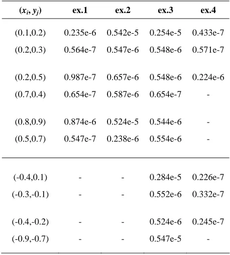
The absolute error of ρn
(
x y,)
−ρ(
x y,)
in some points of function domains for our 4 examples are presented in Table 1.Table 1. Absolute error of examples 1-3 in some points of functions domains
(xi, yj) ex.1 ex.2 ex.3 ex.4
(0.1,0.2) 0.235e-6 0.542e-5 0.254e-5 0.433e-7
(0.2,0.3) 0.564e-7 0.547e-6 0.548e-6 0.571e-7
(0.2,0.5) 0.987e-7 0.657e-6 0.548e-6 0.224e-6
(0.7,0.4) 0.654e-7 0.587e-6 0.654e-7 -
(0.8,0.9) 0.874e-6 0.524e-5 0.544e-6 -
(0.5,0.7) 0.547e-7 0.238e-6 0.554e-6 -
(-0.4,0.1) - - 0.284e-5 0.226e-7
(-0.3,-0.1) - - 0.552e-6 0.332e-7
(-0.4,-0.2) - - 0.524e-6 0.245e-7
(-0.9,-0.7) - - 0.547e-5 -
References
1. Delves L.M. and Mohamad J.L. Computational Methods for Integral Equations. Cambridge University Press, (1985).
3. Razzaghi M. and Yousefi S. Legendre wavelets direct method for variational problems. Mathematics and Computers in Simulation, 53: 185-192 (2000).
4. Keinert F. Wavelets and Multiwavelets. Chapman and Hall/Crc (2004).
5. Kress R. Linear Integral Equations. Springer-Verlage (1989).
6. Baker C.T.H. The Numerical Treatment of Integral Equations. Clarendon Prees, Oxford (1969).
7. Kyythe P.K. and Puri P. Computational Method for Linear Integral Equations. Birkhauser Boston (2002). 8. Babolian E. and Fattahzadeh F. Chebyshev Collocation
Method for Solution of Functional Integral Equations. (Submmited for publication).
9. Babolian E. and Fattahzadeh F. Chebyshev Wavelet Operational Matrix of Integration, (Submmited for publication).
10. Jokar S. Multivariable interpolation by Radial basis functions. M.Sc. Thesis, Sharif University of Thecnology, Tehran, Iran (2003).
11. Davis P. Interpolation and Approximation. Dover Publication, INC. New York (1975).
12. Gasca M. and Sauer T. Polynomial in several variables. Advances in Computational Mathematics, (1999). 13. Kiselman C.O. Approximation by polynomials. Ibid.,
(1999).
14. Schaback R. and Wendland H. Approximation by Positive Definite Kernels. Texed on February 18 (2002). 15. Mairhuber J.C. On Haar’s theorem concerning
Chebyshev approximation problems having unique solutions. Proc. Am. Math. Soc., 7: 609-615 (1956). 16. Wendland H. Scattered Data Modeling by Radial and
Related Functions.Habilitation Thesis, Universität Göttingen (2002).