International Journal of Engineering
J o u r n a l H o m e p a g e : w w w . i j e . i r
Surface Pressure Contour Prediction using a Grnn Algorithm
A. R. Davari*a, M. R. Soltani b, S. Attarian c
a Department of Mechanical and Aerospace Engineering, Islamic Azad University, Science and Research Branch, Poonak, Tehran, Iran b Department of Aerospace Engineering, Sharif University of Technology, Azadi Ave., Tehran, Iran
c Graduate Research Assistant, Islamic Azad University, Science and Research Branch
P A P E R I N F O
Paper history:
Received 04 September 2013
Received in revised form 10 November 2013 Accepted 12 December 2013
Keywords:
GRNN
Leading Edge Vortex Delta Wing Prediction Natural
A B S T R A C T
A new approach based on a Generalized Regression Neural Network (GRNN) has been proposed to predict the planform surface pressure field on a wing-tail combination in low subsonic flow. Extensive wind tunnel results were used for training the network and verification of the values predicted by this approach. GRNN has been trained by the aforementioned experimental data and subsequently was used as a prediction tool to determine the surface pressure. Most of the previous applications of the GRNN in prediction problems were restricted to single or limited outputs, while in the present method the entire planform surface pressure was predicted at once. This highly decreases the calculation time while preserving a remarkable degree of accuracy. The wind tunnel results verify the accuracy of the data offered by the GRNN, which indicates that the present prediction and optimization tool provides sufficient accuracy with modest amount of experimental data.
doi: 10.5829/idosi.ije.2014.27.06c.01
1. INTRODUCTION1
Tight and lower program budgets as well as aggressive schedules today, no longer allow either an extensive wind tunnel test programs as was done in the past or a thorough numerical investigation to study and predict the aerodynamic behavior of flying vehicles. Thus, introduction of an alternative tool enabling to foresee the field aerodynamic properties is of great importance.
Over the past decade, study and utilization of the Artificial Neural Networks (ANNs) has steadily been expanded. ANNs are relatively crude electronic models based on the neural structure of the brain. The brain basically learns from experience. It is natural that some problems beyond the scope of current computers are indeed solvable by small energy efficient packages, called brain modeling. This brain modeling promises a less technical way to develop machine solutions.
The range of practical applications for these networks is indicated by the breadth of studies that have grown out of such diverse backgrounds as biology, computer science, psychology, statistics, etc. This
*Corresponding Author Email: [email protected] (A. R. Davari)
growth is especially evident in engineering community where a wide variety of applications is examined in almost every field of study from control [1], path finding and pattern recognition [2] up to prediction, modeling and optimization problems [3, 4]. Recently, neural networks have been applied to a wide range of aerospace problems, e.g. aerodynamic performance optimization of rotor blade [5], prediction of measured data to enable identification of instrument system degradation [6].
The neural network in fluid mechanics is still a new concept. Little works have been done on this topic comparing other fields. Faller and Schreck [7] used neural networks to predict the real-time three-dimensional unsteady separated flowfields and aerodynamic coefficients of a pitching wing. Lo and Zhao [8] combined the nonlinear neural network methods with conventional linear regression techniques in the wind tunnel force measurements. Berdahl [9] proposed a new application of the neural networks to observe the shock waves in a supersonic channel flow.
aircraft autopilots, flight path simulations, aircraft control systems and component simulations, structural fault detectors, the problem of finding an alternative method for difficult, expensive and time consuming wind tunnel tests still persists and is a real need to predict the behavior of the present and future flying vehicles. Among many attempts to apply the neural network concept in aerospace problems, only in a few cases, the neural networks were used as a prediction tool to estimate the aerodynamic behavior.
In this paper, the authors examined the general regression neural network as a prediction tool for wind tunnel test data. The approach is based on creating an experimental data bank. A neural network is trained by this experimental data. This trained netwrok in the next step is used to extract a reasonable trend from the data and to extend the results to any other cases out of this data bank.
In the different aerodynamic prediction problems already solved by ANN, limited outputs were obtained. Two or three output variables were usually given by the ANN. This paper, addresses a novel approach to predict the surface pressure on a tail planform using the ANNs. The method is sufficiently fast, simple and accurate to predict the aerodynamic variables. Extensive wind tunnel tests have been conducted on a tail-body configuration at different tail deflection angles. Using this data bank, a computer code was developed based on GRNN algorithm to correlate this data base and predict the surface pressure field at any given deflection angle. The results, as will be seen, are in a good agreement with those determined by experiments. The most important advantage of this method is that the entire surface field on the planform can be quickly and accurately determined in each run and the user is just required to specify the deflection angle.
2. MODELS AND EXPERIMENTAL APPARATUS
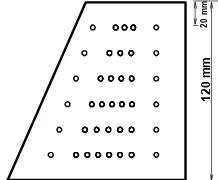
The experiments were performed in a 80 by 80 cm subsonic wind tunnel at a constant velocity of 90 m/sec. The model was a semi body-tail configuration. 64 small pressure tabs were carefully drilled on both the upper and the lower surfaces of the tail. The tail sweep angle was about 20 degrees. The experiments consisted of measuring the tail surface pressure distribution using sensitive pressure transducers for several tail deflection angles. Figures 1 and 2 show the pressure tabs on the tail and the model installed inside the test section.
All data were acquired by an AT-MIO-64E-3 data acquisition board capable of scanning 64 channels at a rate of 500 KHz. The data were then corrected for the wind tunnel sidewalls and the wake blockage effects. An analytical approach [10] was also used to estimate the errors involved in the pressure measurements. Both
the single sample precision and the bias uncertainty in the pressure measurement were estimated. On this basis, the overall uncertainty for the presented data is less than
±%3 [11]. Figure 3 shows the data uncertainties for a typical run.
(a) Tail surface pressure tabs
(b) The model installed in the test section
Figure 1. Model of the half body-tail configuration
Figure 2. Schematic of the pressure tabs position on the upper
surface
Figure 3. Typical measurement uncertainties on the tail upper
surface
1
2
0
m
m
2
0
m
m
x/c cp
0 0.25 0.5 0.75 1
-1 -0.75 -0.5 -0.25 0 0.25 0.5 0.75
a=0
a=10o
3. DESCRIPTION OF THE SUBSONIC FLOWFIELD ON THE BODY-TAIL CONFIGURATION
In an aircraft or missile, the interference problem among the components is of great importance. For the tail-control flying vehicles, the increasingly need towards flying at high angles of attack, without losing the vehicle controllability, requires employing more effective tails. For body-tail configurations, it is desired to obtain a certain amount of lift with an acceptable ratio of the tail deflection angle to the body angle of attack, δ/α. The development of the vortex-like flow on the tail as the tail deflection angle increases, while the body angle of attack is set constantly to zero, is shown in Figure 4. Note that the vortical flow pattern first is appeared near δ=5º, spreads over the surface towards the trailing edge and starts to burst at about δ=17º. At this deflection angle, the vortical flow has been destroyed at the tail outboard region, while the inboard region is still dominated by the vortex. From δ=17º to
δ=30º the burst region gradually covers the entire tail surface [12].
The chordwise pressure distribution at two spanwise sections; y/b=0.3 and y/b=0.7 at zero angle of attack of body and for different tail deflection angles are shown in Figure 5. Both Figures 5(a) and 5(b) approve that the vortical flow is increased in strength and size up to about δ=15º beyond which, the breakdown process starts and the amount of suction on the upper surface decreases. The relatively flat region on the chordwise pressure distribution for δ>20º indicates that nearly 60% of the wing at a spanwise section, y/b=0.3, and about 40% at y/b=0.7 is covered by the burst vortex. Note that the vortex at the outboard region, y/b=0.7, for δ=20º is completely burst while the inboard portion, y/b=0.3, is still dominated by this vortex.
Many theoretical researches were performed to study the role of the lee side vortices on the aerodynamic behavior of the bodies of revolution in low speed subsonic flow at high angles of attack. It has been shown [12] that the lee side vortices on the body are strongly affected by both the wing downwash and the wing sweep angle. Impact of body on the tail flow pattern is depicted in Figure 6. There, the vortex development for zero tail deflection is shown as the body angle of attack increases. From Figure 6, it is evident that the pressure distribution over the tail varies only with angle of attack and is independent of the flow structure over the body for small to moderate body or tail angles up to about 10º. Within the small to moderate deflection angle range means that the surface pressure distribution over the tail remains unaffected, if either the body is set to α≤ 10º at zero tail deflection or the tail is deflected up to 10º at zero body angle of attack. Thus, within small to moderate angle range, no significant viscous effect exists in flow behavior and the flowfiled
over the body does not affect the tail surface pressure distribution. In this situation, the body angle of attack at zero tail deflection and the tail deflection at zero body angle of attack, both have similar effect on the aerodynamic forces and moments developed on the tail. However, this is not true for high angles, even though the net tail angles referenced to the free stream are equal. This is clearly seen in Figure 7, where the pressure distribution at two spanwise sections y/b=0.3 and 0.7 are shown. At low to moderate angles, both Figures 7(a) and 7(c) show that changing the body angle of attack is more efficient than changing the tail deflection in the sense that the suction peak is higher when the body angle of attack changes at zero tail deflection. At 15 degrees deflection angle, where the vortex starts to breakdown, this behavior is different. Near the leading edge, the suction peak associated with the tail deflection is higher due to the body angle of attack. For the rest of the section, the body angle of attack is again appeared to be more effective. For the high angle region of this figure, i.e., Figures 7(b) and 7(d), as stated earlier, the effects of both the body and the tail deflection angles are shown to differ significantly. For 20 degrees angle, the inboard sectional pressure posses a lower suction peak for α=20°
than δ=20°. Returning to Figures 4 and 6, for tail deflection case, a relatively strong vortex is still observed at the inboard section at δ=20º, while this region for the body angle of attack case, α=20°, shown in Figure 6, is nearly disappeared. This is due the nose and body vortices at high angles of attack, which are shed in to the downstream region affecting the tail flow filed. For high deflection angles, once the whole surface is dominated by the burst flow, the favorable effect of body angle of attack comparing to that of tail deflection, is observed again. It seems that the shed vortices from nose and body have a different effect on the tail flowfield at moderated angles where the tail vortex starts to burst and also at high angles where the burst flow covers the entire tail surface. Note from both Figures 7(b) and 7(d) at high angles that increasing the body angle of attack at zero tail incidence also decreases the adverse pressure gradient, inhibiting the flow separation induced by the vortex burst.
4. THE GENERAL REGRESSION NEURAL
NETWORK (GRNN)
(a) δ=0º (b) δ=5º (c) δ=10º
(d) δ=12º (e) δ=15º (f) δ=17º
(g) δ=20º (h) δ=25º (i) δ=30º
Figure 4. Vortical flow developement on the model used in the present experiments [12]
(a) y/b=0.3 (b) y/b=0.7
Figure 5. Effects of tail deflection on the spanwise pressure distribution, α=0 [12]
x/c
y/
b
0 0.2 0.4 0.6 0.8 1 1.2 0 0.1 0.2 0.3 0.4 0.5 0.6 0.7 0.8 0.9 1 1.1 cp 0.7169 0.6182 0.5195 0.4207 0.3220 0.2233 0.1246 0.0259 -0.0729 -0.1716 -0.2703 -0.3690 -0.4678 -0.5665 -0.6652 x/c y/ b
0 0.2 0.4 0.6 0.8 1 0 0.1 0.2 0.3 0.4 0.5 0.6 0.7 0.8 0.9 1 x/c y/ b
0 0.2 0.4 0.6 0.8 1 0 0.1 0.2 0.3 0.4 0.5 0.6 0.7 0.8 0.9 1 x/c y/ b
0 0.2 0.4 0.6 0.8 1 0 0.1 0.2 0.3 0.4 0.5 0.6 0.7 0.8 0.9 1 x/c y/ b
0 0.2 0.4 0.6 0.8 1 0 0.1 0.2 0.3 0.4 0.5 0.6 0.7 0.8 0.9 1 x/c y/ b
0 0.2 0.4 0.6 0.8 1 0 0.1 0.2 0.3 0.4 0.5 0.6 0.7 0.8 0.9 1 x/c y/ b
0 0.2 0.4 0.6 0.8 1 0 0.1 0.2 0.3 0.4 0.5 0.6 0.7 0.8 0.9 1 x/c y/ b
0 0.2 0.4 0.6 0.8 1 0 0.1 0.2 0.3 0.4 0.5 0.6 0.7 0.8 0.9 1 x/c y/ b
0 0.2 0.4 0.6 0.8 1 1.2 0 0.1 0.2 0.3 0.4 0.5 0.6 0.7 0.8 0.9 1 x/c cp
0 0.2 0.4 0.6 0.8 1
-1 -0.8 -0.6 -0.4 -0.2 0 0.2 0.4 0.6 0.8
d= 0o
d= 5o
d= 10o
d= 15o
d= 20o
d= 25o
d= 30o
a= 0 y/b= 0.3
x/c
cp
0.2 0.3 0.4 0.5 0.6 0.7 0.8 0.9 1 -0.8 -0.6 -0.4 -0.2 0 0.2 0.4 0.6 0.8
d=0o
d=5o
d=10o
d=15o
d=20o
d=25o
d=30o
(a) α=5º (b) α =10º (c) α =15º
(d) α =20º (e) α =25º (f) α =30º
Figure 6. Tail pressure contours at various body angles of attack, δ=0 [12]
(a) y/b=0.3, low to moderate angles (b) y/b=0.3, moderate to high angles
(c) y/b=0.7, low to moderate angles (d) y/b=0.7, moderate to high angles
Figure 7. Comparison of the body angle of attack and the tail deflection effects on the tail spanwise pressure distribution [12]
x/c
y/
b
0.2 0.4 0.6 0.8 1 0 0.1 0.2 0.3 0.4 0.5 0.6 0.7 0.8 0.9 1 cp 0.6796 0.5848 0.4899 0.3950 0.3002 0.2053 0.1104 0.0156 -0.0793 -0.1742 -0.2690 -0.3639 -0.4588 -0.5536 -0.6485 x/c y/ b
0 0.2 0.4 0.6 0.8 1
0 0.1 0.2 0.3 0.4 0.5 0.6 0.7 0.8 0.9 1 x/c y/ b
0 0.2 0.4 0.6 0.8 1 0 0.1 0.2 0.3 0.4 0.5 0.6 0.7 0.8 0.9 1 x/c y/ b
0 0.2 0.4 0.6 0.8 1 0 0.1 0.2 0.3 0.4 0.5 0.6 0.7 0.8 0.9 1 x/c y/ b
0 0.2 0.4 0.6 0.8 1 0 0.1 0.2 0.3 0.4 0.5 0.6 0.7 0.8 0.9 1 x/c y/ b
0 0.2 0.4 0.6 0.8 1 0 0.1 0.2 0.3 0.4 0.5 0.6 0.7 0.8 0.9 1 x/c cp
0 0.2 0.4 0.6 0.8 1
-1 -0.8 -0.6 -0.4 -0.2 0 0.2 0.4
0.6 a=5o,d=0o
a=10o,d=0o
a=15o,d=0o
d=5o,a=0o
d=10o,a=0o
d=15o,a=0o
x/c
cp
0 0.2 0.4 0.6 0.8 1
-1 -0.8 -0.6 -0.4 -0.2 0 0.2 0.4 0.6 0.8
a=20o,d=0o
a=25o,d=0o
a=30o,d=0o
d=20o,a=0o
d=25o,a=0o
d=30o,a=0o
x/c
cp
0.2 0.3 0.4 0.5 0.6 0.7 0.8 0.9 1 -1 -0.8 -0.6 -0.4 -0.2 0 0.2 0.4
0.6 a=5o,d=0o
a=10o,d=0o
a=15o,d=0o
d=5o,a=0o
d=10o,a=0o
d=15o,a=0o
x/c
cp
0.2 0.3 0.4 0.5 0.6 0.7 0.8 0.9 1 -0.8 -0.6 -0.4 -0.2 0 0.2 0.4 0.6 0.8
a=20o
,d=0o a=25o,d=0o a=30o
Figure 8. A GRNN block diagram [13]
(a) Low to moderate incidences
(b) Moderate to high incidences
Figure 9. Variations of mean error with the smoothness
parameter at different incidences
The General Regression Neural Network (GRNN) was first introduced by Donald Specht in 1991 [13]. The GRNN architecture consists of an input layer followed by three computational layers: pattern, summation and
output layers. When an input pattern is presented at the input layer, the pattern layer units compute the Euclidean distance between its weight vector and the input vector. This distance is then transformed by the unit’s activation function, which are exponential (Gaussian) functions [14].
In a prediction problem such as aerodynamic modeling, the number of neurons in the input layer is equal to the number of input variables, and the number of neurons in the output layer is the same as the number of predicted variables [13]. The block diagram of a GRNN is for prediction problems is shown in Figure 8, where f(x,y) represents the known joint continuous probability density function of a vector random variable, x, and a scalar random variable, y and Ŷ is the predicted output for an input .
Selection of the rest of the architecture in the network in terms of the number of neurons in the hidden layer, the learning rate, etc., is not pre-known. Thus, one has to resort to trial and error methods to find a suitable network structure for a given problem [15].
GRNN presents a nonlinear prediction method, which has several advantages to other usual prediction methods in mathematics. The conventional prediction methods usually use either of the following strategies; in the first method, a function of a specific form is chosen for a specific problem having several unknowns, which may be a polynomial, sinusoidal, Bessel, Fourier, etc. Using the observed outputs from this function and applying the statistical methods, the unknowns are determined and a model will be obtained for the problem under consideration. The main problem with this method is that it needs try and error. For an incorrect choice of the initial function, the prediction process will be very complicated.
The second method is to use a general polynomial form for the function, i.e. for predicting the function under consideration, the order of the polynomial and the number of the independent variables are first specified. The unknown coefficients will then be determined using the observed outputs from the system. For the complicated problems with higher order polynomials and considerable number of the unknown coefficients, this method is usually inapplicable.
Both methods may be known as parametric prediction schemes since the base of both is to predict some unknown parameters. However, as stated, GRNN uses non-parametric estimators and needs no predefined function. This network, directly applies the training inputs and outputs for prediction. With a proper choice of the smoothness parameter, σ, to be discussed in the next sention, GRNN can use the modest data to correlate the inputs and outputs. For this reason, GRNN needs only a few data to predict the simple functions such as sigmoid and with increasing the training data, it can predict every nonlinear, complicated and even
s
M
e
a
n
E
rr
o
r
0 0.1 0.2 0.3 0.4 0.5 0.6 0.7 0.8 0
0.04 0.08 0.12 0.16 0.2 0.24
d=5o
d=10o
d=12o
s
M
e
a
n
E
rr
o
r
-0.1 0 0.1 0.2 0.3 0.4 0.5 0.6 0.7 0.8 0
0.2 0.4 0.6
d=15o
d=20o
chaotic functions [15].
The smoothness parameter controls the adaptation level of the network to the desired function. Large values of σ, increases the averaging process in the network and is desirable for the functions with shallow oscillations. It also reduces the noises encountered in the prediction process, while small values for σ enable the network to simulate the complicated and oscillatory functions. Large amount of calculations to determine the estimated output is the only disadvantage of GRNN. However, the problem may be alleviated by proper clustering the input space for training data.
In the present investigation, the surface pressure data on a tail planform measured in the wind tunnel were used to train a GRNN. The input to this network was the deflection angle and the position of the pressure tabs, while the output was the pressure distribution on the surface at the given incidence. The network, once being trained by the surface pressure field at different incidence angles, can predict the pressure distribution over the same planform at different angles of attack.
Eventhough the experiments were conducted for both cases of different model angles of attack at zero tail incidence and different tail incidence angles at zero model angle of attack, only the data for various tail incience angles with zero model angle of attack was used to train the data. As shown earlier, these two cases are different especially at moderate to high angles where nose and forebody vortex shedding come into play.
5. NETWORK TRAINING IN THE PRESENT INVESTIGATION USING THE EXPERIMENTAL DATA
There are actually two usual methods to choose σ, which as stated before, plays a vital role in the prediction accuracy and the performance of a GRNN. Specht [13] suggests the holdout method to select the proper value of σ. In this method, one sample from the entire set is removed and for a fixed σ, GRNN is used again to predict this sample with the remainder set of training samples. The squared difference between the predicted value of the removed training sample and the training sample itself is then calculated and stored. If the removed sample is designated by (Xj, Yj), the network error in predicting Yj must be calculated.
The process of removing samples and predicting them again for the selected value for σ is repeated for each sample. After this procedure, the mean of the squared differences is calculated for each run. The process is repeated for several values of σ. The σ for which, the sum of the mean squared difference is a minimum for all of the mean squared differences, is the
proper choice and should be used for the predictions by this set of training samples.
The holdout method works with very small values of the smoothness parameters [13]. Therefore, the evaluation of the exponential function causes numerical problems, even for a 64-bit data storage.
The second usual method to determine the proper value for σ is known as the wiggle-method [16], which is purely empirical and works for any arbitrary dimensions. In this method, it is necessary to consider the proper number of additional inflections to account for unequally spaced data or measurement errors. For the wiggle method, GRNN predicts the curve over the entire range of the data. σ is originally chosen to be very small, too small to predict the curve without wiggles. The value of σ is then increased by a constant step until the number of inflection points is reached to its allowable limit.
The smoothness parameter, σ, must be chosen in such a manner that the mean estimation error be a minimum. The wiggle method mentioned earlier to determine the smoothness parameter is not a good choice if the training data exhibit a nonlinear and complex behavior. This is really the case for the present data including vortex formation, growth and burst and its interactions with nose and fore body flowfield. For this reason, in the present work, the holdout method was employed to determine the smoothness parameter for the experimental data base developed by the authors.
Figure 9 shows the variations of the mean estimation error with the smoothness parameter for various angles of incidence on the aforementioned model to find the most convenient value for the smoothness parameter.
There is a distinct difference between the behavior at low and high angles, i.e. the trend for δ=5 through 12 degrees is different from that of δ=15 degrees and higher. The vortex burst phenomenon at about δ=17 degrees observed in Figure 4, may be a reason for this behavior.
The mean error is overally higher at moderate to high incidences than that at low to moderate. Furthermore, for δ=15° (just prior to burst onset at
δ=17°) the mean error is higher than δ=20° and 25°
(after burst). In low incidence region as the tail incidence angle increases, the mean prediction error variations with the smoothness parameter decreases. However, for data correlation and regression in the next section, the smoothness parameter at each angle of incidence was chosen to be the one, which minimizes the mean estimation error.
6. GRNN PREDICTED DATA
various spanwise locations for δ=10º, where the vortex-like flow is still active and attached on the surface. The data predicted by the GRNN are compared with those measured in the wind tunnel. The vortex signature in this figure is the suction peak extending from near the leading edge at the root to near the trailing edge at the tip. Excellent agreement is observed between the predicted and the measured data for the points away from the vortex core. However, in the core region, where the suction suction peak lies, some discrepancies are observed, which decreases as moving towards the outboard sections.
Figure 10. Chordwise pressure distribution comparison at
δ=10º
Figure 11. Chordwise pressure distribution comparison at
δ=17º
Figure 12. Chordwise pressure distribution comparison at
δ=20º
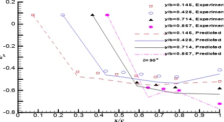
Figure 13. Chordwise pressure distribution comparison at
δ=30º
In Figure 11, the pressure distribution is presented for δ=17º, where according to Figure 4(f) vortex burst occurs and the burst flow covers more than half of the span of the planform. In this case, the suction peak has been disappeared and in the absence of this low prssure region, good accuracy can be observed in the predicted data. Even though the burst point has reached the half span section, the pressure distribution on both the inboard and the outboard sections of the planform has been successfully predicted by the GRNN. For higher incidences, i.e. δ=20º and δ=30º, where the separated flow dominates, Figures 12 and 13 show that the prediction accuracy is still remarkable. However, since most of the training data were in the attached flow region, in the range of δ less that 17 degrees, the pressure predicted by GRNN in the burst region, where
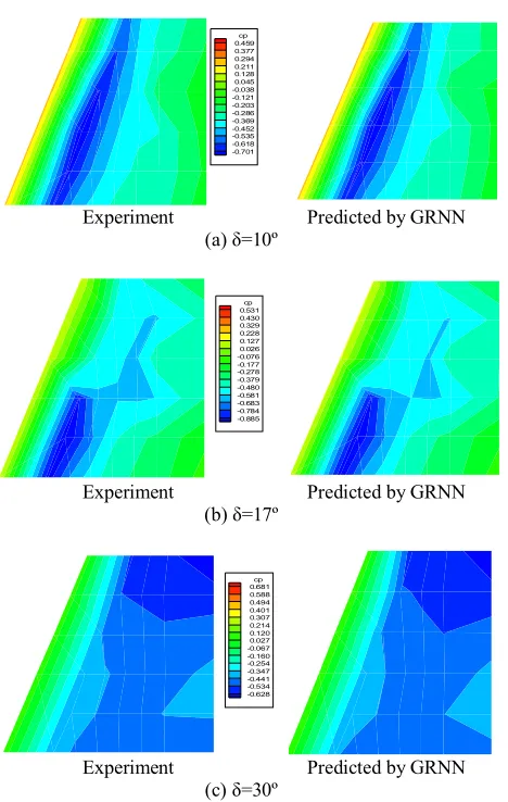
δ>17, is a little different from those measured in the wind tunnel. Once the flow is burst, the suction peak either is disappeared or becomes weak. However, the GRNN cannot foresee and apply this change in the pressure distribution accurately. Instead, the network predicted a small suction for the cases where the bust flow is dominated. The error encountered by this weak prediction is not large and seems to be improved if more experimental data for high incidence cases are used to train the network. In Figure 14, the surface pressure contours have been compared for both the experimental and predicted data for various tail deflection angles. As observed earlier, the pressure contours predicted by the GRNN are very similar in shape to those obtained from the wind tunnel results. Even the burst phenomenon in Figure 14(b), which is usually difficult to predict by the classic analytical and numerical tools, has successfully been predicted by the GRNN. The separated flow at high angles of attack observed in Figure 14(c) is also predicted with a high accuracy by this method.
This reveals the vital role of the smoothness parameter in this problem. The network could predict the data in high incidence region with the training data mostly were in low and moderate range.
x/c
cp
0 0.2 0.4 0.6 0.8 1
-0.8 -0.6 -0.4 -0.2 0 0.2 0.4 0.6 0.8
d=10o
y/b=0.145, E xperiment y/b=0.428, E xperiment y/b=0.714, E xperiment y/b=0.857, E xperiment y/b=0.145, P redicted y/b=0.428, P redicted y/b=0.714, P redicted y/b=0.857, P redicted
x/c
cp
0.2 0.3 0.4 0.5 0.6 0.7 0.8
-1 -0.8 -0.6 -0.4 -0.2 0
d=17o
y/b=0.145, E xperiment y/b=0.428, E xperiment y/b=0.714, E xperiment y/b=0.857, E xperiment y/b=0.145, P redicted y/b=0.428, P redicted y/b=0.714, P redicted y/b=0.857, P redicted
x/c
cp
0.2 0.3 0.4 0.5 0.6 0.7 0.8
-1 -0.8 -0.6 -0.4 -0.2 0
d=20o
y/b=0.145, Experiment y/b=0.428, Experiment y/b=0.714, Experiment y/b=0.857, Experiment y/b=0.145, Predicted y/b=0.428, Predicted y/b=0.714, Predicted y/b=0.857, Predicted
x/c cp
0 0.1 0.2 0.3 0.4 0.5 0.6 0.7 0.8 0.9 1 -0.8
-0.6 -0.4 -0.2 0 0.2
d= 3 0o
Experiment Predicted by GRNN (a) δ=10º
Experiment Predicted by GRNN
(b) δ=17º
Experiment Predicted by GRNN
(c) δ=30º
Figure 14. Comparison of experimental and GRNN predicted
pressure contours
As stated earlier, large values of σ, increases the averaging process in the network and is desirable for the functions with shallow oscillations, while small values for σ enable the network to simulate the complicated and oscillatory functions. The problem of surface pressure pattern prediction on a swept planeform, encompasses both high and low gradient regions depending on the position under consideration on the planform and incidence angle. Thus, the smoothness parameter for each tail incidence angle should be chosen according to the flow characteristics and the level of pressure variations in that incidence angle.
7. CONCLUSION
A series of wind tunnel tests were performed on a tail-body configuration in subsonic flow at different tail incidence angles to study the tail flow field in the
presence of the body. The results were used to train a Generalized Regression Neural Network. This network, once being trained, can accurately predict the surface flow field on the tail at any given angles.
The data predicted by GRNN in low to moderate tail incidence angles show an excellent accuracy comparing to the experimental results. This is beacause most of the training data were in this region where the flow is attached. However, in the regions on the wing where the vortex suction peak lies, some discrepancies were observed between the predicted and experimental values.
At higher tail incidences, once the flow is burst, the trained GRNN could not accurately simulate the fast and sharp changes occurred in the flowfield. Consequently, small differences can be observed between the predicted flowfield and the experimental data at high incidence region. Though, the overal error encountered by predictions in high incidence angle region and those near the vortex core on the planform process were not remarkable to improve the accuracy in such conditions. Thus, more data in those region should be used to train the network. However, this algorithm has been shown to present a good accuracy with a minimum training data in this region.
8. REFERENCES
1. Mori, R. and Suzuki, S., "Neural network modeling of lateral pilot landing control", Journal of Aircraft, Vol. 46, No. 5, (2009), 1721-1726.
2. Basu, J.K., Bhattacharyya, D. and Kim, T.-h., "Use of artificial neural network in pattern recognition", International Journal of Software Engineering & Its Applications, Vol. 4, No. 2, (2010).
3. Austin, N., Kumar, P.S. and Kanthavelkumaran, N., "Artificial neural network involved in the action of optimum mixed refrigerant (domestic refrigerator)", International Journal of Engineering (1025-2495), Vol. 26, No. 10, (2013)
4. Deswal, S. and Pal, M., "Artificial neural network based modeling of evaporation losses in reservoirs", Proceedings of World Academy of Science: Engineering & Technology, Vol. 41, (2008)
5. WALSH, J. and ROGERS, J., "Aerodynamic performance optimization of a rotor blade using a neuralnetwork as the analysis", (1992).
6. McMillen, R.L., Steck, J.E. and Rokhsaz, K., "Application of an artificial neural network as a flight test data estimator", Journal of aircraft, Vol. 32, No. 5, (1995), 1088-1094.
7. Faller, W.E. and Schreck, S.J., "Real-time prediction of unsteady aerodynamics: Application for aircraft control and manoeuvrability enhancement", Neural Networks, IEEE Transactions on, Vol. 6, No. 6, (1995), 1461-1468.
8. Lo, C.F., Zhao, J.L. and DeLoach, R., "Application of neural networks to wind tunnel data response surface methods", in 21 st AIAA Aerodynamics Measurement Technology and Ground Testing Conference, (2000), 19-22.
cp 0.459 0.377 0.294 0.211 0.128 0.045 -0.038 -0.121 -0.203 -0.286 -0.369 -0.452 -0.535 -0.618 -0.701
cp 0.531 0.430 0.329 0.228 0.127 0.026 -0.076 -0.177 -0.278 -0.379 -0.480 -0.581 -0.683 -0.784 -0.885
9. Berdahl, C., "Neural network detection of shockwaves", AIAA journal, Vol. 40, No. 3, (2002), 531-536.
10. Rae, W.H. and Pope, A., "Low-speed wind tunnel testing, John Wiley, (1984)
11. Beckwith, T.G., Marangoni, R.D. and Lienhard, J.H., "Mechanical measurements, Pearson Prentice Hall, (2007) 12. Davari, A.R., Hadi Dulabi, M., Soltani, M.R. and Askari, F.,
"Impact of body on the tail surface flowfield at high incidences",
Journal of Aerospace Science and Technology; JAST, Vol. 6, No. 1, (2009)
13. Specht, D.F., "A general regression neural network", Neural Networks, IEEE Transactions on, Vol. 2, No. 6, (1991), 568-576.
14. Parzen, E., "On estimation of a probability density function and mode", Annals of mathematical statistics, Vol. 33, No. 3, (1962), 1065-1076.
15. Cacoullos, T., "Estimation of a multivariate density", Annals of the Institute of Statistical Mathematics, Vol. 18, No. 1, (1966), 179-189.
16. Bauer, M.M., "General regression neural network for technical use", Master's Thesis, University of Wisconsin-Madison, (1995).
Surface Pressure Contour Prediction using a Grnn Algorithm
A. R. Davaria, M. R. Soltani b, S. Attarian c
a Department of Mechanical and Aerospace Engineering, Islamic Azad University, Science and Research Branch, Poonak, Tehran, Iran b Department of Aerospace Engineering, Sharif University of Technology, Azadi Ave., Tehran, Iran
c Graduate Research Assistant, Islamic Azad University, Science and Research Branch
P A P E R I N F O
Paper history:
Received 04 September 2013
Received in revised form 10 November 2013 Accepted 12 December 2013
Keywords:
GRNN
Leading Edge Vortex Delta Wing Prediction Natural
هﺪﯿﮑﭼ
ﺪﯾﺪﺟشورﮏﯾﻪﻟﺎﻘﻣﻦﯾارد
ﺑﺮ
ﯽﻋﻮﻨﺼﻣﯽﺒﺼﻋﻪﮑﺒﺷيﺎﻨﺒﻣ
GRNN
رﺎﺸﻓﻊﯾزﻮﺗناﻮﺗﯽﻣنآيﺎﻨﺒﻣﺮﺑﻪﮐهﺪﯾدﺮﮔدﺎﻬﻨﺸﯿﭘ
دﻮﻤﻧﯽﻨﯿﺑﺶﯿﭘتﻮﺻﺮﯾزنﺎﯾﺮﺟردنﺎﻣﺰﻤﻫرﻮﻃﻪﺑﺢﻄﺳﻞﮐيورارﯽﻟﺮﺘﻨﮐﮏﻟﺎﺑﮏﯾﺢﻄﺳيور
.
وﻪﮑﺒﺷشزﻮﻣآﺖﻬﺟ
ﻪﻧﺪﺑﺐﯿﮐﺮﺗﮏﯾيوردﺎﺑﻞﻧﻮﺗردﯽﯾاهدﺮﺘﺴﮔيﺎﻫﺶﯾﺎﻣزآ،هﺪﺷﯽﻨﯿﺑﺶﯿﭘﺞﯾﺎﺘﻧﺖﺤﺻﯽﺳرﺮﺑ
-ﮏﯾومﺎﺠﻧاﯽﻟﺮﺘﻨﮐﮏﻟﺎﺑ
ﮏﻧﺎﺑ
ﺪﯾدﺮﮔﻦﯾوﺪﺗنآﺞﯾﺎﺘﻧزاﯽﺗﺎﻋﻼﻃا
.
ﻪﮑﺒﺷزاهدﺎﻔﺘﺳاﺎﺑ ﻦﯿﻤﺨﺗ لﻮﻤﻌﻣﻞﺋﺎﺴﻣ رد
GRNN
ﺪﻨﭼﺎﯾﮏﯾﻻﻮﻤﻌﻣ،
دﻮﺷﯽﻣجاﺮﺨﺘﺳاﻪﮑﺒﺷﻦﯾازادوﺪﻌﻣﯽﺟوﺮﺧ
.
نﺎﯾﺮﺟناﺪﯿﻣﻦﯿﻤﺨﺗﻪﻟﺎﻘﻣﻦﯾاردهﺪﺷهدﺎﻔﺘﺳاﻢﺘﯾرﻮﮕﻟاتﻮﻗطﺎﻘﻧزاﯽﮑﯾ
ﺮﺑ ﻦﯿﻋرد ﻪﮐﺖﺳانﺎﻣﺰﻤﻫ وﻞﻣﺎﮐرﻮﻃﻪﺑ ﮏﻟﺎﺑﺢﻄﺳ يور
ﻦﮑﻤﻣ نﺎﻣزﻦﯾﺮﺗهﺎﺗﻮﮐ رد،ﺐﺳﺎﻨﻣ ﺖﻗدزا يرادرﻮﺧ
ﺪﻧﺎﺳرﯽﻣمﺎﺠﻧاﻪﺑارﻪﻃﻮﺑﺮﻣتﺎﺒﺳﺎﺤﻣ
.
ﻦﯿﻤﺨﺗﺞﯾﺎﺘﻧﻪﺴﯾﺎﻘﻣ
GRNN
ﺪﯿﯾﺎﺗارﻦﯿﻤﺨﺗﺞﯾﺎﺘﻧﺖﻗد،دﺎﺑﻞﻧﻮﺗيﺎﻫدادو
ﺪﻧاهدﻮﻤﻧ
.
doi: 10.5829/idosi.ije.2014.27.06c.01
![Figure 5. Effects of tail deflection on the spanwise pressure distribution, α=0 [12]](https://thumb-us.123doks.com/thumbv2/123dok_us/232335.2017827/4.595.69.527.111.531/figure-effects-tail-deflection-spanwise-pressure-distribution-a.webp)
![Figure 7. Comparison of the body angle of attack and the tail deflection effects on the tail spanwise pressure distribution [12]](https://thumb-us.123doks.com/thumbv2/123dok_us/232335.2017827/5.595.90.533.415.729/figure-comparison-attack-deflection-effects-spanwise-pressure-distribution.webp)
![Figure 8. A GRNN block diagram [13]](https://thumb-us.123doks.com/thumbv2/123dok_us/232335.2017827/6.595.62.282.314.640/figure-grnn-block-diagram.webp)