MARKOVIAN SOFTWARE RELIABILITY MODEL FOR TWO
TYPES OF FAILURES WITH IMPERFECT DEBUGGING RATE
AND GENERATION OF ERRORS
M. Jain
Department of Mathematics, IIT, Roorkee- 247667 (India)
[email protected], [email protected]
S. C. Agrawal, P. Agarwal*
School of Basic and Applied Sciences, Shobhit University, Meerut-250001, (India)
[email protected], [email protected]
*Corresponding Author
(Received: November 25, 2010 – Accepted in Revised Form: January 19, 2012) doi:10.5829/idosi.ije.2012.25.02a.07
Abstract
This investigation deals with a software reliability model based on Markov process. For formulating the model, we define a random variable representing the cumulative number of faults successfully corrected upto a specified point of time. This model is based on the assumption that there are two types of software failures. Further the concepts of imperfect debugging environment and error generation phenomenon are taken into consideration. Transient analysis based on Laplace transform and matrix approach has been done to find the solution of the system of differential difference equations. Several performance indices for software reliability assessment are derived for this model. Numerical results with the help of Runge-Kutta Method show that the proposed framework incorporating both concepts of imperfect debugging phenomenon and error generation for two types of faults has a fairly accurate prediction capability.
Keywords Software reliability; Imperfect debugging; Error generation; Markov process; Software reliability growth.
هﺪﯿﮑﭼ
يراﺰﻓا مﺮﻧ لﺪﻣ ﮏﯾ ﺖﯿﻠﺑﺎﻗ ﯽﺳرﺮﺑ ﻪﺑ ﻪﻟﺎﻘﻣ ﻦﯾا سﺎﺳا ﺮﺑ
ﺪﻨﯾاﺮﻓ فﻮﮐرﺎﻣ ﯽﻣ دزادﺮﭘ . ياﺮﺑ ﻪﻟﻮﻣﺮﻓ
شور ندﺮﮐ ،
ﺮﯿﻐﺘﻣ ﮏﯾ ﯽﻓدﺎﺼﺗ
زا ﯽﮔﺪﻨﯾﺎﻤﻧ ﻪﺑ داﺪﻌﺗ
ﺎﺑ ﻪﮐ ﯽﯾﺎﻫﺎﻄﺧ ﻞﮐ ﺖﯿﻘﻓﻮﻣ
رد ﻪﻄﻘﻧ ﮏﯾ نﺎﻣز زا ﺺﺨﺸﻣ
ﺖﺳا هﺪﺷ ﺢﯿﺤﺼﺗ ﻢﯿﻨﮐ ﻒﯾﺮﻌﺗ
. لﺪﻣ ﻦﯾا ﺮﺑ سﺎﺳا ﯽﻣ ضﺮﻓ ﻦﯾا ﺪﺷﺎﺑ
: ود عﻮﻧ ﺖﺴﮑﺷ زا راﺰﻓا مﺮﻧ
دﻮﺟو دراد .
ﻦﯾا ﺮﺑ هوﻼﻋ ﻢﯿﻫﺎﻔﻣ
ﻂﯿﺤﻣ ﯽﯾادز لﺎﮑﺷا ﺺﻗﺎﻧ
ﺎﻄﺧ دﺎﺠﯾا هﺪﯾﺪﭘ و
ﺮﻈﻧ رد ﻪﺘﻓﺮﮔ هﺪﺷ ﺖﺳا . ارﺬﮔ ﺰﯿﻟﺎﻧآ ﺮﺑ
سﺎﺳا سﻼﭘﻻ ﻞﯾﺪﺒﺗ و
شور ﺲﯾﺮﺗﺎﻣ ندﺮﮐ اﺪﯿﭘ ياﺮﺑ ﻞﺣ هار
ﻢﺘﺴﯿﺳ ﻞﺿﺎﻔﺗ تﻻدﺎﻌﻣ هﺪﺷ مﺎﺠﻧا ﯽﻠﯿﺴﻧاﺮﻔﯾد
ﺖﺳا . يداﺪﻌﺗ زا يدﺮﮑﻠﻤﻋ يﺎﻫ ﺺﺧﺎﺷ ياﺮﺑ
ﯽﺑﺎﯾزرا نﺎﻨﯿﻤﻃا ﺖﯿﻠﺑﺎﻗ راﺰﻓا مﺮﻧ
لﺪﻣ ﻦﯾا ياﺮﺑ ﺖﺳا هﺪﺷ ﻖﺘﺸﻣ
.
ﺞﯾﺎﺘﻧ يدﺪﻋ ﮏﻤﮐ ﺎﺑ شور ﻪﮕﻧار ﺎﺗﻮﮐ ﺪﻫد ﯽﻣ نﺎﺸﻧ ﻪﮐ
بﻮﭼرﺎﭼ يدﺎﻬﻨﺸﯿﭘ
ياﺮﺑ ﺐﯿﮐﺮﺗ ﺮﻫ ود مﻮﻬﻔﻣ هﺪﯾﺪﭘ
ﯽﯾادز لﺎﮑﺷا ﺪﯿﻟﻮﺗ و ﺺﻗﺎﻧ
ﺎﻄﺧ ياﺮﺑ ود عﻮﻧ ﺎﻄﺧ ياراد ﺖﯿﻠﺑﺎﻗ ﯽﻨﯿﺑ ﺶﯿﭘ ﺎﺘﺒﺴﻧ
ﻖﯿﻗد يﺮﺗ ﺖﺳا .
1. INTRODUCTION
Software engineers generally need a period of time to read, and analyze the collected software failure data. Software reliability models based on stochastic process have gained wide acceptance in the software industry because they are useful engineering tools to analyze and to correct the faults. Software reliability estimates are generally made by building probability models of data
related models available in the literature related to SRGMs. For the first time Jelinski and Moranda [11] introduced such a model. Later in the field of software engineering similar models were attempted by Musa [17] and Shooman [20] and many others. Tokuno and Yamada [22] discussed the modeling of markovian software availability in their exhaustive research article. Non-Homogeneous markov reward model for a multi-state system reliability assessment with different assumptions was developed by Whittaker et al. [27], Lisnianski [13], Lisnianski et al. [15], Lisnianski and Frenkel [14]. Hamlet et al. [8] studied component based software reliability theory. Gokhale and Trivedi [5] discussed analytical models for architecture-based software reliability prediction. Dohi et al. [3] developed software reliability assessment models based on cumulative Bernoulli trial processes. Prowell and Poore [18]] computed system reliability using markov chain usage models. Chung and Ortega [2] analyzed the error tolerant motion estimation. Ravishanker et al. [19] studied NHPP models with markov switching for software reliability. Jalote et al. [10] discussed post-release reliability growth in software products. Huang and Hung [9] analyzed software reliability assessment using queueing models with multiple change-points. Recently in [4] Dulz et al. gave a polyhedron approach to calculate probability distributions for markov chain usage models.
In the case of software reliability, two major issues confound to estimate software reliability, i.e. imperfect debugging and error generation. This concept in a software reliability modeling is a controversial issue. No real world software company possesses infinite resources to test and correct every software fault in the real world. However, a Markov model approach in this regard may be worthwhile and useful to deal with such a situation.
There are several reasons for using NHPP models or hazard rate models in a specific situation. Generally, models are developed for the analysis of failure data collected during the testing stage then we develop our model analytically with the help of NHPP models or hazard rate models. These group of models provides an analytical framework for describing the software failure phenomenon during testing phase and with the help of these group of models we can estimate the
future behavior of the software system.
One common assumption of conventional software reliability modeling is that the detected faults are immediately removed; but this assumption may not be realistic in actual software development. In reality, most latent faults may remain uncorrected for a very long time, even after they are detected by professional testers, which increase their impact. Kapur et al. [12] obtained the transient solution of a software reliability model with imperfect debugging and error generation. Yamada et al. [28] did the software reliability measurement in imperfect debugging environment and also discussed its application. Gokhale et al. [6] developed a non-homogeneous markov software reliability model with imperfect repair. Sridharan and Jayashree [21] considered a transient solution of a software model with imperfect debugging and generation of errors by two servers. Tokuno and Yamada [23]] studied a markovian software reliability model with a decreasing perfect debugging rate. Tokuno and Yamada [24] established the imperfect debugging model with two types of hazard rates for software reliability measurement and assessment. Tokuno and Yamada [25] suggested the markovian software reliability measurement with geometrically decreasing perfect debugging rate. Tokuno and Yamada [26] proposed the relationship between software availability measurement and the number of restorations with imperfect debugging. Gupta and Singh [7] estimated software reliability by sequential testing with simulated annealing of mean field approximation. Mathematical modeling of software reliability testing with imperfect debugging was discussed by Cai et al. [1]. Meedeniya et al. [16] derived reliability deployment optimization technique for embedded systems.
results are obtained in section 5 with the help of R-K and matrix method. To explore the effects of different parameter, the sensitivity analysis is also carried out. Finally conclusions are drawn in section 6.
2. MODEL DESCRIPTION
A stochastic model is sought that represents the injection (due to the occurrence of development and debugging errors) and removal (due to successful repairs) of software. The stochastic behavior of the fault correction phenomenon with imperfect debugging is described by a Markov process. In this investigation, we assume that there exist two types of faults in the software such as (i) Due to originally latent in the system before
the testing.
(ii) Due to generated during the testing phase and the error generation phenomenon never leads the software to having infinite errors.
We develop a software model by making the following assumptions:
The software has a finite number of two types of faults; there are m faults of type I whereas n faults of type II.
The probability that two or more software failures occur simultaneously is negligible. The failure rate is proportional to the number
of fault remaining in the software.
The debugging process is performed as soon as the software failure occurs.
When the debugging process is performed, at most one fault is corrected and the fault correction time is considered negligible. The maximum number of faults in the
software never exceeds a finite limit, i.e., m<M, n<N.
When a failure occurs, an instantaneous repair effort starts and the following cases arise;
(i). The fault content function is reduced by one for type I faults with probability p0.
(ii). The fault content function remains unchanged for type I faults with probability p1.
(iii). The fault content function is increased by one for type I faults with probability p2.
(iv). The fault content function is reduced by one for type II faults with probability q0.
(v). The fault content function remains unchanged for type II of faults with probability q1.
(vi). The fault content function is increased by one for type II faults with probability q2.
The debugging activity is performed without distinguishing between both types of faults.
Notations
α : Failure rate per remaining software fault for type I faults.
β : Failure rate per remaining software fault for type II faults.
m : Initial fault content for I type of faults. M : Maximum fault content for I type of faults. n : Initial fault content for the II type of faults. N : Maximum fault content for II type of faults. Fij(t):Probability that there are i(j) faults of type I (II) in the software at time t. where i 0 i M and j 0 j N
2.1. Governing Equations The transient equations governing the model are constructed by considering the transition flow rates. The differential difference equations associated with
0 0( ) 0 10( ) 0 01( )
F t p F t q F t (1)
0 1 0 2 ( 1)0
0 ( 1)0 0 1
( ) ( ) 1 ( )
1 ( ) ( ), 2 1
i i i
i i
F t i i p F t i p F t
i p F t q F t i M
(2)
0 0 0 2 0 0 ( 1) 0
0 1 1
( ) 2 ( )
( ),
i i i i
i i
F t p F p F p F t
q F t
(3)
0( ) 0 0( ) 1 2 1 0( )
M M M
F t Mp F t M p F t (4)
0 0 0 2 0 0 1,
0 0 ( 1) 1
( ) ( ) ( ) ( )
2 ,
j j j j
j j
F t q F t q F t p F t
q F
(5)
0 1 0 2 0 1
0 1, 0 0( 1)
( ) ( ) 1 ( )
( ) 1 , 2 1
j j j
j j
F t j j q F t j q F t
p F t j q F j N
(6)
0N( ) 0 0N( ) ( 1) 2 0(N 1)( )
F t N q F t N q F t (7)
1 1 1 1 2 11
2 ( 1)1 0 2
( ) ( ) ( )
1 ( ) ( ), 2 2
i i
i i
F t q i i p F t p F t
i p F t i q F t i M
1 0 0 2 2 1
2 ( 1)1 0 2
( ) ( )
2 ( ) 2 ( ), 1
i i
i i
F t p q p q F t
p F t q F t i
(9)
0 01 1 1 1
2 ( 2)1
( ) 1 ( )
2 ( )
M M
M
F t q M p F t
M p F t
(10)
1 1 1 1
2 1( 1) 0 2
0 1( 1)
( ) ( )
1 ( ) 2 ( )
1 ( ), 2 j N-2
j j
j j
j
F t p j j q F t
j q F t p F t
j q F t
(11)
0 01 1 1 1
2 1( 2)
( ) 1 ( )
2 ( )
N N
N
F t p N q F t
N q F t
(12)
1 12 ( 1) 2 ( 1)
0 ( 1) 0 1
( ) ( )
1 ( ) 1 ( )
1 ( ) 1 , 2
i j i j
i j i j
i j i j
F t i i p j j q F t
i p F j j q F t
i p F t j q F t j
(13)
0 02 1 2 3, 2
1
1 ,
ij ij ij
ij
i j i M j N
F t i p F t i q F t
i q F t i p F t
(14)
0 02 1 2 2, 3
1
1 ,
ij ij ij
ij
i j i M j N
F t i p F t i q F t
q F t i p F t
(15)
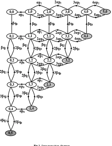
2.2. Illustration In this section, for illustration purpose we present a markov model for two types of errors where maximum number of faults of each type are five (i.e. M=N=5). The differential difference equations related to this particular case are as follows:
00( ) 0 10( ) 0 01( )
F t p F t q F t (16)
10( ) 1 10( ) 2 0 20( ) 0 11( )
F t p F t p F t q F t (17)
20 1 20 2 10
0 30 0 21
( ) 2 2 ( ) ( )
3 ( ) ( )
F t p F t p F t
p F t q F t
(18)
30 1 30 2 20
0 4 0 0 31
( ) 3 3 ( ) 2 ( )
4 ( ) ( )
F t p F t p F t
p F t q F t
(19)
40 1 4 0 2 30
0 50 0 41
( ) 4 4 ( ) 3 ( )
5 ( ) ( )
F t p F t p F t
p F t q F t
(20)
50( ) 5 0 50( ) 4 2 40( )
F t p F t p F t (21)
01 1 01 0 0 2 0 11 (22)
11 1 1 11
0 12 0 21
( ) ( )
2 ( ) 2 ( )
F t q p F t
q F t p F t
(23)
21 1 1 21
2 11 0 2 2 0 31
( ) 2 2 ( )
( ) 2 ( ) 3 ( )
F t q p F t
p F t q F t p F t
(24)
31 1 1 31
2 21 0 32 0 41
( ) 3 3 ( )
2 ( ) 3 ( ) 4 ( )
F t q p F t
p F t q F t p F t
(25)
41( ) 0 4 0 41( ) 3 2 31( )
F t q p F t p F t (26)
0 2 1 0 2 2 01
0 03 0 12
( ) 2 2 ( ) ( )
3 ( ) ( )
F t q F t q F t
q F t p F t
(27)
12 1 1 12
2 11 0 13 0 2 2
( ) 2 2 ( )
( ) 3 ( ) 2 ( )
F t q p F t
q F t q F t p F t
(28)
2 2 1 1 2 2
2 21 0 23 0 32 2 12
( ) 2 2 2 2 ( )
( ) 3 ( ) 3 ( ) ( )
F t q p F t
q F t q F t p F t p F t
(29)
32 0 0 32 2 31
2 2 2
( ) 3 3 ( ) ( )
2 ( )
F t q p F t q F t
p F t
(30)
03 1 03 2 0 2
0 0 4 0 13
( ) 3 3 ( ) 2 ( )
4 ( ) ( )
F t q F t q F t
q F t p F t
(31)
13 1 1 13
2 12 0 14 0 23
( ) 3 3 ( )
2 ( ) 4 ( ) 2 ( )
F t q p F t
q F t q F t p F t
(32)
23 0 0 23 2 2 2
2 13
( ) 3 2 ( ) 2 ( )
F t q p F t q F t
p F t
(33)
0 4 1 0 4 2 03
0 0 5 0 14
( ) 4 4 ( ) 3 ( )
5 ( ) ( )
F t q F t q F t
q F t p F t
(34)
14( ) 4 0 0 14( ) 3 2 13( )
F t q p F t q F t (35)
05( ) 5 0 05( ) 4 2 04( )
F t q F t q F t (36)
3. THE SOLUTION APPROACH
We denote the Laplace transform of f tij( ) byf sij( ). For solving the set of equations governing the (16)-(36) and solve using matrix method with initial conditionsfk(0) 1, (0) 0 fn for nk.
F (t)
q F
(t) 2q F (t) p F (t)Fig 1. State transition diagram
0,0
1,0
2,0
3,0
4,0
5,0
αp
0βq
00,1
1,1
2,1
3,1
4,1
2
β
q
0βq
20,2
1,2
2,2
3,2
2
β
q
20,3
1,3
2,3
3
β
q
23
β
q
00,4
1,4
0,5
4
β
q
05
β
q
04
β
q
2αp
0αp
0αp
0αp
02
α
p
03
α
p
04
α
p
05
α
p
0αp
22
α
p
23
α
p
24
α
p
2αp
2αp
2αp
22
α
p
02
α
p
02
α
p
03
α
p
03
α
p
04
α
p
02
α
p
23
α
p
22
α
p
2βq
0βq
0βq
0βq
02
β
q
02
β
q
02
β
q
03
β
q
03
β
q
04
β
q
03
β
q
22
β
q
22
β
q
20 10( ) 0 01( ) 1
p F s q F s
(37)
0 2 0 0 11
1 10
2 ( ) ( )
( ) 0
p F s q F s
s p F s
(38)
2 10 0 30 0 21
1 2 0
( ) 3 ( ) ( )
2 2 ( ) 0
p F s p F s q F s
s p F s
(39)
2 2 0 0 4 0 0 31
1 30
2 ( ) 4 ( ) ( )
3 3 ( ) 0
p F s p F s q F s
s p F s
(40)
2 30 0 50 0 41
1 4 0
3 ( ) 5 ( ) ( )
4 4 ( ) 0
p F s p F s q F s
s p F s
(41)
2 40 0 50
4p F ( )s s 5p F ( ) 0s
(42)
0 0 2 0 11 1 01
2q F ( )s p F s( ) s q F ( ) 0s
(43)
0 12 0 21
1 1 11
2 ( ) 2 ( )
( ) 0
q F s p F s
s q p F s
(44)
2 11 0 2 2 0 31
1 1 21
( ) 2 ( ) 3 ( )
2 2 ( ) 0
p F s q F s p F s
s q p F s
(45)
2 21 0 32 0 41
1 1 31
2 ( ) 3 ( ) 4 ( )
3 3 ( ) 0
p F s q F s p F s
s q p F s
(46)
2 31 0 0 41
3p F ( )s s q 4p F ( ) 0s
(47)
2 01 0 03 0 12
1 0 2
( ) 3 ( ) ( )
2 2 ( ) 0
q F s q F s p F s
s q F s
(48)
2 11 0 13 0 2 2
1 1 12
( ) 3 ( ) 2 ( )
2 2 ( ) 0
q F s q F s p F s
s q p F s
(49)
2 21 0 23 0 32 2
12 1 1 2 2
( ) 3 ( ) 3 ( )
( ) 2 2 2 2 ( ) 0
q F s q F s p F s p
F s q p F s
(50)
2 31 2 2 2
0 0 32
3 3 ( )
s q p F s
(51)
2 12 0 14 0 23
1 1 13
2 ( ) 4 ( ) 2 ( )
3 3 ( ) 0
q F s q F s p F s
s q p F s
(53)
2 2 2 2 13
0 0 23
2 ( ) ( )
3 2 ( ) 0
q F s p F s
s q p F s
(54)
2 03 0 05 0 14
1 0 4
3 ( ) 5 ( ) ( )
4 4 ( ) 0
q F s q F s p F s
s q F s
(55)
2 13 0 0 14
3q F ( )s s 4q p F ( ) 0s
(56)
2 0 4 0 05
4q F ( )s s 5q F ( ) 0s
(57)
For brevity, we denote the probabilities Fi j, and Laplace transform of probabilities Fi j,
s with single suffix i.e. by Fi as defined and F si
, respectively below:
,0 1, ,0 1 , 0 5
i i i i
F F F s F s i ;
,1 6 1, ,1 6 1 , 0 4
i i i i
F F F s F s i ;
,2 11 1, ,2 11 1 , 0 3
i i i i
F F F s F s i ;
,3 15 1, ,3 15 1 , 0 2
i i i i
F F F s F s i ;
,4 18 1, ,4 18 1 , 0 1
i i i i
F F F s F s i ;
,5 21, ,5 21i i
F F F s F s
Q( ). ( )s F s F 0
(58)
where, F s
and F
0 are the column vector i.e.,
1
, 2 ,... 21
T
F s F s F s F s and 0
1,0,0,..., 0
TF
Also Q(s) is matrix given by
1 2
3 4 5
6 7 21 21 0 Q( )
0
A A
s A A A
A A
i
2q F2 0 2(s)4q F0 0 4(s)p F0 13(s)
s 3 3 q F (s) 0
Here submatrices A (i=1,2,……9) are constructed for particular case as follows:
(52)
1
03 q F (s)2p F (s)
0
0 0 1 02 1 0
2 1 0
2 1 0
2 0
1 1
0 0 0 0
0 2 0 0 0 0
0 2 2 3 0 0 0
0 0 2 3 3 4 0 0
0 0 0 3 4 4 5 0
0 0 0 0 4 5 0
0 0 0 0 0 0
s p q
s p p
p s p p
p s p p
A
p s p p
p s p
s q
1 0 0
2 2 0 0
2 3 0
2 0 0
1 0
2 4 0
2 2 5
4
2 0 0 0 2 0
3 0 0 0 2
0 2 4 0 0 0
0 0 3 4 0 0 0
0 0 0 0 2 2 0
0 0 0 0 2
0 0 0 0
s p q
p s p q
p s p
A p s q p
s q p
q s p
q p s
0 01 0 0
6 0 0
2 0 0
2 1 0 0
2 0 0
2 0
7
3 3 0 0 0 0 0 0
0 3 3 0 4 0 0
0 0 2 0 4 0
0 0 3 2 0 0 0
0 3 0 0 4 4 5
0 0 3 0 0 4 0
0 0 0 0 4 0 5
s q p
s q p q
s p q
A p s q p
q s q p q
q s q p
q s q
0 0 2 0 0 0 0
0 0 0 0 0 0 0
0 0 0 0 0 0
0 0 0 0 0 0
0 0 0 0 0 0
0 0 0 0 0 0
0 0 0 0 0 0 0
0 0 0 2 0 0
q q A q q p q 3 2
0 0 0 0 0 0 0
0 0 0 0 0 0 0
0 0 0 0 0 0 0
0 0 0 0 0 0 0
0 0 0 0 0 0
0 0 0 0 0 0 0
0 0 0 0 0 0 0
A q 0 5 0 0 0
0 0 0 0 0 0 0
0 0 0 0 0 0 0
3 0 0 0 0 0 0
0 0 0 0 0 0 0
0 3 0 0 0 0 0
0 0 3 0 0 0 0
0 0 0 3 0 0 0
q A q q q 2 2 2 2 2 6
0 0 0 0 0 2
0 0 0 0 2 0 0
0 0 0 0 0 2 0
0 0 0 0 0 0 2
0 0 0 0 0 0 0
0 0 0 0 0 0 0
0 0 0 0 0 0 0
For brebiely of notations, in sub matrices, we have used
1
1 1
i q i p
, i=1, 2, 3
1 1
1 1
i i q p
, i=4, 5, 6
Using Cramer’s rule, the probabilitiesF sk
, canbe obtained as
1( ), 0 ( )k k
Q s
F s k L
Q s
(59)
For calculating the characteristic roots of the matrix Q(s), we note that
s = 0 is one of the roots. Let s = -d, so that we get
Q d QdI (60)
. ( )
( )
0Q d F s QdI F s F (61)
It may be observed that the eigen values of Q are real and distinct and Q is positive definite. So, all eigen values of Q are positive. Let k
1 k L
denotes the eigen values of Q, then we get
1
( ) L k
k
Q s s s
(62) so that1 k
1 ( )
( ) , 1 k
( )
l L
k k
Q s
F s L
s s
(63)
We may expand F sk( )by partial fractions, i.e., in
the form
0 01
1
L k
k k
a a
F s
s s
(64)
k k
1
( ) L j
j j
a F s
s
, k2,3,...,L (65)
where a0and an(n=1,2,…..L) are real numbers
calculated as 1 0
1 (0)
L j j
Q a
(66) and
1
1
( )
, 1 , 2
l k lk L
k j k j
k
Q
a l L k L
(67)and (60), we get
1 1
1
1
1 1
(0) ( ) exp( )
( ) L k k
L L
k
k k j k
k j
k
Q Q t
F t
(68)
1 1
1
( ) exp( )
( ) L l k k , 2
l L
k
k j k
j k
Q t
F t where l L
(69)
4. PERFORMANCE INDICES
Now we give some performance measures for the quantification of software reliability indices as follows:
The probability of a perfect program at time t is given by F1(t).
The mean number of faults remaining in the software at time t is given as
1
L i i
E D t iF t
(70) The software reliability is defined as
1exp
L i
i i
R x t F t x
(71)5. SENSITIVITY ANALYSIS
Since no live data is available so instead of estimating the parameters we have used the secondary data for validity and practical utility of our model (Ref. Kapur et al. 1992).
In this section, we perform computational experiment for the transient analysis by employing Runge-Kutta technique (RKT) of fourth order and matrix method to solve the system of differential equations. R-K method is implemented by exploiting MATLAB’s ‘ode45’ function. A time span is considered with equal intervals. Eigen On taking inverse Laplace transform of Eqs (59)
On inverting Eq (63), we have
values are evaluated by the using MATLAB’6.5 software. For illustration purpose, we choose default parameters as 0.49, 0.02, p0=0.6, p1=0.3, p2=0.1,q0=0.5, q1=0.3, and q2=0.2.
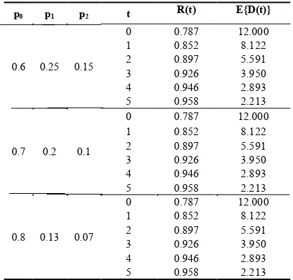
From Tables 1 and 2, we notice the patterns of various performance indices namely R(t) and E{D(t)} by varying the probabilities p0, p1, p2 and q0, q1, q2, respectively. It is observed that there is an increasing trend in the values of R(t) and decreasing trend in E{D(t)} with the increasing values of p0and q0.
Table 1.Software reliability and E{D(t)} for different values of p0, p1and p2.
p0 p1 p2 t R(t) E{D(t)}
0.6 0.25 0.15
0 0.787 12.000
1 0.852 8.122
2 0.897 5.591
3 0.926 3.950
4 0.946 2.893
5 0.958 2.213
0.7 0.2 0.1
0 0.787 12.000
1 0.852 8.122
2 0.897 5.591
3 0.926 3.950
4 0.946 2.893
5 0.958 2.213
0.8 0.13 0.07
0 0.787 12.000
1 0.852 8.122
2 0.897 5.591
3 0.926 3.950
4 0.946 2.893
5 0.958 2.213
Table 2.Software reliability and E{D(t)} for different values of q0, q1and q2.
q0 q1 q2 t R(t) E{D(t)}
0.6 0.3 0.1
0 0.787 12.000
1 0.858 7.848
2 0.904 5.227
3 0.933 3.596
4 0.951 2.589
5 0.963 1.971
0.7 0.2 0.1
0 0.787 12.000
1 0.868 7.238
2 0.917 4.494
3 0.945 2.944
4 0.961 2.078
5 0.969 1.596
0.8 0.13 0.07
0 0.787 12.000
1 0.880 6.542
2 0.930 5.591
3 0.956 3.950
4 0.968 2.893
5 0.974 2.213
The effects of failure rates α and β on I and II type faults, are shown in Tables 3 and 4. As expected, reliability R (t) increases with testing time whereas decreases with the increase in the failure rate α. Mean number of remaining faults decreases as testing time increases but remains same for the increasing values of failure rate α.
Table 3.Performance indices for different values of α.
α=0.01 α =0.03 α =0.05 t R(t) E{D(t)} R(t) E{D(t)} R(t) E{D(t)}
0 0.698 12.000 0.549 12.000 0.432 12.000
1 0.796 7.848 0.691 7.848 0.603 7.848
2 0.862 5.227 0.787 5.227 0.724 5.227
3 0.903 3.596 0.850 3.596 0.803 3.596
4 0.929 2.589 0.889 2.589 0.852 2.589
5 0.945 1.971 0.913 1.971 0.883 1.971
6 0.955 1.593 0.928 1.593 0.902 1.593
7 0.961 1.362 0.937 1.362 0.914 1.362
Table 4.Performance indices for different values of β.
β=0.5 β =0.6 β =0.7
t R(t) E{D(t)} R(t) E{D(t)} R(t) E{D(t)}
0 0.000 12.000 0.000 12.000 0.000 12.000
1 0.071 7.848 0.073 7.524 0.074 7.215
2 0.167 5.227 0.166 4.832 0.164 4.473
3 0.240 3.596 0.233 3.238 0.223 2.929
4 0.289 2.589 0.275 2.303 0.258 2.067
5 0.321 1.971 0.300 1.757 0.279 1.590
6 0.340 1.593 0.315 1.439 0.290 1.326
7 0.352 1.362 0.324 1.255 0.296 1.180
Fig 2a. Probability of perfect program at time t by
varying α.
Fig 2b.Probability of perfect program at time t by
varying β.
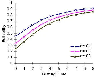
Figs 3a and 3b are plotted for the reliability by varying α and β for I and II type of faults, respectively. From Fig 3a, we notice that the reliability decreases as α increases. But in Fig 3b, initially reliability increases with the testing time and remains almost same with the increasing the value of β.
Fig 3a.Software reliability by varying α
Fig 3b.Software reliability by varying β
From Figs 4a and 4b, mean number of remaining faults E{D(t)} has been examined by varying the parameters α and β. It is seen that E{D(t)} decreases as time increases but remains same for all values of α and β.
Fig. 4a.Mean number of faults remainingby varying α.
Fig. 4b.Mean number of faults remainingby varying β.
Overall, with the help of numerical results we observe that the optimal release time of the software can be determined successfully. For
0 0.1 0.2 0.3 0.4 0.5 0.6 0.7 0.8 0.9 1
0 10 20 30 40 50 60 70 80
Testing Time
F
1
(t
)
β=.150
β=.165
β=.180 0
0.1 0.2 0.3 0.4 0.5 0.6 0.7 0.8 0.9 1
0 10 20 30 40 50 60 70 80
Testing Time
F
1
(t
)
α=.3
α=.5
α=.7
0 0.1 0.2 0.3 0.4 0.5 0.6 0.7 0.8 0.9 1
0 1 2 3 4 5 6 7 8 9
Testing Time
R
e
li
a
b
il
it
y
β=0.5
β=0.6
β=0.7
0 0.1 0.2 0.3 0.4 0.5 0.6 0.7 0.8 0.9 1
0 1 2 3 4 5 6 7 8 9
Testing Time
R
e
li
a
b
il
it
y
α=.01
α=.03
α=.05
0 2 4 6 8 10 12 14
0 1 2 3 4 5 6 7 8 9
Testing Time
E
{D
(t
)}
α=.01
α=.02
α=.03
0 2 4 6 8 10 12 14
0 1 2 3 4 5 6 7 8 9
Testing Time
E
{D
(t
)}
β=.95
β=.97
example, if the initial error content function is assumed to be 12, we can notice from the Figs 4a and 4b that E{D(t)} ≤ 12. This means that the software developer can decide the time to a specific software quality level with the condition that the reliability may reach at a maximum level. Similar conclusions for other performance measures are also evident from the other figures and tables.
Based on the sensitivity analysis which has been given in this paper, one can estimate the idea about the release time of the software. For example, from Tables 9.3 and 9.2, we see that as remaining faults in the software are becoming less then reliability of the software is increasing and finally it became constant that shows the real situation of testing the software. In that sense, the markovian software reliability model with imperfect debugging and generation of errors proposed in this paper are intuitively understandable and can provide to a software developer a more tractable framework for developing a real time situation assessment tools in spite of their simple structure.
6. CONCLUSION
In this paper, we have developed the markovian software reliability model by including the concept of imperfect debugging and error generation phenomenon. The suggested approach is suitable for practical application in reliability engineering. Our stochastic model provides a theoretical framework during the software development for understanding the factors that affect the software reliability. The suggested model may be helpful in measuring and assessing the software reliability, during operational phase.
7. REFERENCES
1. Cai, K.-Y., Cao, P., Dong, Z. and Liu, K. (2010): Mathematical modeling of software reliability testing with imperfect debugging, Computers & Mathematics
with Applications, Vol. 59, No. 10, 3245-3285.
2. Chung, H. and Ortega, A. (2005): Analysis and testing for error tolerant motion estimation, In Proceeding of International Symposium on Defect and Fault
Tolerance in VLSI Systems, 514-522.
3. Dohi, T., Yasui, K. and Osaki, S. (2003): Software reliability assessment models based on cumulative Bernoulli trial processes, Mathematical and Computer
Modelling, Vol. 38, 1177-1184.
4. Dulz, W., Holpp, S. and German, R. (2010): A Polyhedron Approach to Calculate Probability Distributions for Markov Chain Usage Models,
Electronic Notes in Theoretical Computer Science,
Vol. 264, No. 3, 19-35.
5. Gokhale, S. S. and Trivedi, K. S. (2006): Analytical models for architecture-based software reliability prediction: a unification framework, IEEE
Transactions on Reliability, Vol. 55, No. 4, 578-590.
6. Gokhale, S. S., Philip, T. and Marinos, P. N. (1996): A non-homogeneous markov software reliability model with imperfect repair, In Proceeding of International
Performance and Dependability Symposium.
7. Gupta, N. and Singh, M. P. (2006): Estimation of software reliability by sequential testing with simulated annealing of mean field approximation, International Journal of Engineering, Transactions B: Applications, Iran, Vol. 19, No. 1, 35-44.
8. Hamlet, D., Woit, D. and Mason, D. (2001): Theory of software reliability based components, In Proceeding of
International Conference on Software Engineering,
361-370.
9. Huang C.-Y. and Hung, T.-Y. (2010): Software reliability analysis and assessment using queueing models with multiple change-points, Computers &
Mathematics with Applications, Vol. 60, No. 7,
2015-2030.
10. Jalote, P., Murphy, B. and Sharma, V. S. (2008): Post-release reliability growth in software products, ACM
Transactions on Software Engineering and
Methodology, Vol. 17, No. 4, 17.1-17.20.
11. Jelinski, Z. and Moranda, P. B. (1972): Software reliability research, Statistical Computer Performance
Evaluation, New York, 468-484.
12. Kapur, P. K., Sharma, K. D. and Garg, R. B. (1992): Transient solution of a software reliability model with imperfect debugging and error generation,
Microelectronics and Reliability, Vol. 38, No. 4,
475-478.
13. Lisnianski, A. (2007): The markov reward model for a multi-state system reliability assessment with variable demand, Quality Technology & Quantitative
Management, Vol. 4, No. 2, 265-278.
14. Lisnianski, A. and Frenkel, I. (2009): Non-Homogeneous markov reward model for aging multi state system under minimal repair, International
Journal of Performability Engineering, Vol. 5, No. 4,
303-312.
15. Lisnianski, A. and Frenkel, I., Khvatskin, L. and Ding, Y. (2007): Markov reward model for multi state system reliability assessment, Statistical models and Methods
for Biomedical and Technical Systems, 153-168.
16. Meedeniya, I., Buhnova, B., Aleti, A. and Grunske, L. (2011): Reliability-driven deployment optimization for embedded systems, Journal of Systems and Software,
Vol. 84, No. 5, 835-846.
Engineering, SE-1, 312-327.
18. Prowell, S. J. and Poore, J. H. (2004): Computing system reliability using markov chain usage models,
The journal of Systems and Software, Vol. 73,
219-225.
19. Ravishanker, N., Liu, Z. and Ray, B. K. (2008): NHPP models with markov switching for software reliability,
Computational Statistics and Data Analysis, Vol. 52,
3988-3999.
20. Shooman, M. L. (1977): Software reliability: analysis and prediction, Report AGARD AG224, Integrity in
Electronic Flight Control Systems, 1-17.
21. Sridharan, V. and Jayashree, P. R. (1998): Transient solution of a software model with imperfect debugging and generation of errors by two servers, Mathematical
and Computing Modelling, Vol. 27, No. 3, 103-108.
22. Tokuno, K. and Yamada, S. (1999a): A summary of markovian software availability modeling, In Proceeding of Fifth ISSAT International Conference
Of Reliability and Quality in Design, (Edited by Pham,
H. and Lu, M.-W.), 218-222.
23. Tokuno, K. and Yamada, S. (1999b): A markovian software reliability model with a decreasing perfect debugging rate, In proceeding First Western Pacific and Third Australia-Japan Workshop on Stochastic
Models in Engineering, Technology and Management, (Edited by Wilson, R. J., Osaki, S. and Faddy, M. J.), 528-536.
24. Tokuno, K. and Yamada, S. (2000): An imperfect debugging model with two types of hazard rates for software reliability measurement and assessment,
Mathematical and Computing Modelling, Vol. 31,
343-352.
25. Tokuno, K. and Yamada, S. (2003a): Markovian software reliability measurement with a geometrically decreasing perfect debugging rate, Mathematical and
Computing Modelling, Vol. 38, 1443-1451.
26. Tokuno, K. and Yamada, S. (2003b): Relationship between software availability measurement and the number of restorations with imperfect debugging,
Computers and Mathematics with Applications, Vol.
46, 1155-1163.
27. Whittaker, J. A., Rekab, K. and Thomson, M. G. (2000): A markov chain model for predicting the reliability of multi-build software, Information and Software
Technology, Vol. 42, 889-894.
28. Yamada, S., Tokuno, K. and Osaki, S. (1993): Software reliability measurement in imperfect debugging environment and its application, Reliability