Finite Capacity Queuing System with Vacations and Server Breakdowns

FINITE CAPACITY QUEUEING SYSTEM WITH VACATIONS

AND SERVER BREAKDOWNS

R.P. Ghimire and Ritu Basnet*

Department of Mathematics, School of Science, Kathmandu University, Dhulikhel (Nepal) [email protected], [email protected]

*Corresponding Author

(Received: October 08, 2009 – Accepted in Revised Form: October 20, 2011)

doi:10.5829/idosi.ije.2011.24.04a.07

Abstract This paper deals with finite capacity single server queuing system with vacations. Vacation starts at rate if the system is empty. Also, the server takes another vacation if upon his arrival to the system, finds the system empty. Customers arrive in the system in Poisson fashion at rate₀during vacation, faster rate_fduring active service and slower rate_s 0during the breakdown. Customers are served exponentially with the rate. Server breakdowns at rate b and it is immediately repaired exponentially with the rater. We derive the explicit formulas for queue length distribution, average queue length, average number of customers in the system and average waiting time for a customer in queue, and in the system. Numerical illustrations have been cited to show that the proposed model is practically sound.

Keywords Multiple–vacation, Server breakdowns, Repair, Generating functions, Average queue length.

1. INTRODUCTION

Several researchers [1- 4] studied the queuing systems with server vacations and obtained various measures of performance. Takagi [5] studied M/G/1/N queue with server vacations and exhaustive service and obtained the distributions of the unfinished work, the virtual waiting time and the real waiting time, etc. Wang [6] proposed an N- policy M/M/1 queueing system with server breakdowns and obtained analytic closed-form solutions. Takine and Sengupta [7] obtained the queue-length distribution and waiting time distribution of a single-server queue under the provision of service interruptions. Boxma et al.[8] studied the length of a vacation and steady-state

workload distribution, both for single and multiple vacations. Ke [9] proposed M/G/1 queuing system with server vacations, startup and breakdowns and obtained the system total expected cost function per unit time under optimal control mechanism. Zhang et al.[10] analyzed of an M/M/1/N queue with balking, reneging and server vacations and derived the matrix form solution of the steady-state probabilities and formulated a cost model to determine the optimal service rate. Wang et al.

[11] made a comparative analysis between the exact results and the maximum entropy results, also illustrated through the maximum entropy results that the maximum entropy principle approach is accurate enough for practical purposes. Jain and Agrawal [12] studied the Mx_/M/1 ﺪﻧﺍﻩﺪﺷﻪﺋﺍﺭﺍﻥﺁﺩﺮﮑﻠﻤﻋ ﺖﺤﺻﻥﺩﺍﺩﻥﺎﺸﻧﻱﺍﺮﺑﻱﺩﺎﻬﻨﺸﻴﭘﻝﺪﻣ

ﺯﺍﻞﺻﺎﺣﻱﺩﺪﻋﺕﺎﻔﻴﺻﻮﺗﻭﺞﻳﺎﺘﻧ .ﺩﻮﺷﻲﻣﺝﺍﺮﺨﺘﺳﺍﻲﻫﺩﺲﻳﻭﺮﺳﺭﺩﻭﻒﺻﺭﺩﻱﺮﺘﺸﻣﮏﻳﻱﺍﺮﺑﺭﺎﻈﺘﻧﺍﻥﺎﻣﺯ ﻂﺳﻮﺘﻣﻭ ،ﻢﺘﺴﻴﺳﺭﺩ ﻱﺮﺘﺸﻣ r ﺩﺍﺪﻌﺗ ﻂﺳﻮﺘﻣ ،ﻒﺻ ﻝﻮﻃ ﻂﺳﻮﺘﻣ،ﻒﺻ ﻝﻮﻃ ﻊﻳﺯﻮﺗﻱﺍﺮﺑ ﺢﻳﺮﺻﻝﻮﻣﺮﻓ ﻪﻟﺎﻘﻣ ﻦﻳﺍﺭﺩ .ﺪﻧﻮﺷﻲﻣﻲﺑﺎﻳﺯﺎﺑ ﺥﺮﻧﺎﺑﻲﻳﺎﻤﻧﺕﺭﻮﺻ ﻪﺑ ﹰﺍﺭﻮﻓﻭs،ﺏﺍﺮﺧ b ﺥﺮﻧﺎﺑﺎﻫﻩﺪﻨﻫﺩﺲﻳﻭﺮﺳ .ﺪﻧﻮﺷﻲﻣ

λ ≥0 f

ﻲﻫﺩﺲﻳﻭﺮﺳµ ﺥﺮﻧ ﺎﺑﻲﻳﺎﻤﻧ ﺕﺭﻮﺻﻪﺑﻥﺎﻳﺮﺘﺸﻣ0 .ﺪﺷﺎﺑﻲﻣ ﺥﺮﻧ ﺎﺑﻲﺑﺍﺮﺧﻥﺎﻣﺯﺭﺩﻭ؛ λ ﺮﺗﻊﻳﺮﺳ ﺥﺮﻧﮏﻳﺎﺑﻝﺎﻌﻓﻲﻫﺩﺲﻳﻭﺮﺳﻲﻃﺭﺩ؛ λ ﺥﺮﻧﺎﺑﻲﺼﺧﺮﻣﻲﻃﺭﺩﺩﻭﺭﻭﻦﻳﺍﻪﮐﻱﺍﻪﻧﻮﮔﻪﺑﺪﻧﻮﺷﻲﻣﻢﺘﺴﻴﺳ ﺩﺭﺍﻭﻥﻮﺳﺍﻮﭘ ﻊﻳﺯﻮﺗ ﺎﺑﻥﺎﻳﺮﺘﺸﻣ .ﺩﺮﻴﮔﻲﻣ ﻱﺮﮕﻳﺩﻲﺼﺧﺮﻣﺪﻨﻴﺒﺑ ﻲﻟﺎﺧ ﺍﺭﻒﺻﻪﮐﻲﺗﺭﻮﺻ ﺭﺩ،ﻢﺘﺴﻴﺳﻪﺑ ﻩﺪﻨﻫﺩ ﺖﻣﺪﺧﺩﻭﺭﻭ ﺾﺤﻣﻪﺑ ﻦﻴﻨﭽﻤﻫ .ﺩﻮﺷﻲﻣ ﻉﻭﺮﺷυ ﺥﺮﻧﺎﺑﻲﺼﺧﺮﻣ ،ﺪﺷﺎﺑ ﻲﻟﺎﺧ ﻢﺘﺴﻴﺳﻪﮐ ﻲﺗﺭﻮﺻﺭﺩ .ﺪﺷﺎﺑ

queueing system with multiple types of server breakdown under N-policy and provided the numerical results to demonstrate the effects of various parameters on the system performance characteristics. Ke and Wang [13] analyzed the operating characteristics for the heterogeneous batch arrival queue with startup and breakdown and performed a sensitivity analysis among the optimal value of N, specific values of system parameters, and the cost elements of Mx_/M/1

queue. Srivastava and Jain [14] analyzed an optimal N-policy model for single Markovian queue with breakdown repair and state dependent arrival rate and obtained steady state for various operational characteristic and optimal value of N under a linear cost structure. Hur and Paik [15] analyzed the effect of different arrival rates on the N- policy of M/G/1 with server setup and derived the distribution function of the steady state queue length, waiting time using Laplace Stieltjes transform. Ke and Pearn [16] studied the management policy of M/M/1 queueing service system with heterogeneous arrivals under the N policy, in which the server is characterized by breakdowns and vacations and derived the distribution of the system size and mean queue length. Gray et al. [17, 18] studied the vacation queueing model with service breakdown under the assumption of different arrival rates and obtained formulas for queue length distribution and the mean queue length for M/M/1.

The queuing system with vacations and server breakdowns in infinite capacity system can be found in several research papers but from the practical view point this system may not always be the case .In many real life situations the finite capacity system plays the vital role such as in customized manufacturing systems, maintenance activities, and telecommunication network centers where the multi-task employees are to be deployed. In this paper we investigate finite capacity queueing system with multiple vacations and server breakdowns. The server completely stops serving customers during a vacation and start serving whenever number of customers N (≥1) in the system. Once service starts, there can be an interruption due to server breakdown, and it is sent to repair facility. As soon as the repair process completes, the server starts to serve the same interrupted customer.

2. MATHEMATICAL MODEL AND ANALYSIS

 (0, )i is the state in which there are icustomers in the queue and the server is on vacation,

0 i N. Its probability isp 0 i( , ).

 (1, )i is the state in which there areicustomers

in the system during active service, 1 i N  . Its probability is ( , )p 1 i .

 (2, )i is the state in which there areicustomers in the system during repair process, 1 i N  . Its probability isp(2, )i .

The generating function for the queue length distribution is

0

( ) ( ) _f( ) _s( )

F z F z F z F z (1) where the partial generating functions are:

,

N N N

i i i

0 f s

i=0 i=1 i=1

F (z)=



p(0,i)z , F (z)=



p(1,i)z F (z)=



p(2,i)z

The balance equations for the queue length distribution are:

0

λ p(0,0)=μp(1,1) (2)

0 0

(λ +υ)p(0,i) =λ p(0,i - 1) 1 i N  (3)

0

υp(0,N)=λ p(0,N - 1) (4)

f

(λ +μ+b)p(1,1)=υp(0,1)+μp(1,2)+ rp(2,1) (5)

f f

(λ +μ+b)p(1,i) =λ p(1,i - 1)

+υp(0,i)+μp(1,i+1)+ rp(2,i), 2 i N  (6)

f

(μ+b)p(1,N) =λ p(1,N - 1)+υp(0, N)+ rp(2,N) (7)

s

(λ +r)p(2,1)= bp(1,1) ₍₈₎

s s

(λ + r)p(2,i)= bp(1,i)+λ p(2,i - 1), 2 i < N (9)

s

rp(2,N)= bp(1,N)+λp(2,N - 1) (10)

Equation (2) gives

0

λ

p(1,1)= p(0,0).

μ

(11)

0

λ

p(0,N)= p(0,N - 1)

υ (12) Substituting (11) into (8), we obtain:

0

s s

bλ

b

p(2,1) = p(1,1) = p(0,0)

λ + r μ(λ + r)

(13)

From Equation (3), we get:

i 0

p(0,i)=ρ p(0,0), 1≤iN (14)

where 0 0 0 λ ρ = λ +υ

From Equations (12) and (14), we get:

N i 0

i=0

F (z) =



p(0,i)z =

N

N -1 N

0 0

0 0

1 - (ρ z) λ

+ ρ z p(0,0) 1 - (ρ z) υ

 

 

 

(15)

Multiplying Equation (6) by

z

iand summing for 2,3, , 1

i  N





f f f

N

N -1 N

0 0 0 0 0 2 s μ

μ+b - -λ(z - 1) F (z)= (λ +μ+b)p(1,1)z z

1-(ρ z) λ

+υ + ρ z - 1-ρz p(0,0) 1-(ρ z) υ

μ

- p(1,1)z+ p(1,2)z +rF (z)- rp(2,1)z. z             (16)

Now, we find F zs( )in terms ofF zf( ), then using Equation (16), we find F zf( ). Multiply Equation

(9) by

z

i_{and sum for i2,3, ,N1}



s f

s s

b

F (z)= F (z)

(λ + r - zλ )

(17)

Substituting the (17) into (16), we get





N 0

f f

s s 0

N -1 N 2

0

0 0

1-(ρ z)

(z - 1)Q(z)

F (z)= (λ +μ+b)p(1,1)z +υ +

z(λ+ r -λz) 1-(ρ z)

λ μ

ρ z - 1-ρz p(0,0)- p(1,1)z+ p(1,2)z - rp(2,1)z

υ z       (18) where 2

f s f s f s s s

Q(z)=λ λ z -(λ λ + λ r +bλ + μλ )z + μ(r + λ ) (19)

In order for the queue length distribution to exist, the R.H.S. of Equation (18) must vanish when z=1. Since p(1,1)andp(2,1) are given, now we find

μp(1,2)

f s N N -1 0 0 0 0 0 rb

μp(1,2)= λ +b - p(1,1) λ + r

1-ρ λ

+ ρ - 1-ρ p(0,0)

1-ρ υ

              (20)

Substituting (20) into (18)

f

s s

(z - 1)Q(z)

F (z)=μ(z - 1)p(1,1) z(λ + r - λ z)

N+1 N 2 N N 2

0 0 0

0 0

N -1 N 0 0

ρ (z - z )-ρ (z - z)+ρ(z - 1) -(z - 1) +υ

(1-ρ )(1 -ρz)

p(0,0)+λ ρ (z - z)p(0,0)+υ(z - 1)p(0,0)

      (21) or, f 0 s s

Q(z) _{F (z)= (λ +υ)zp(0,0)+υ}

(λ + r - λ z)

N+1 N +1 2 N 2

0 0 0 0 0

0 0

ρ Φ(z) - ρ z - ρ Φ(z)+ ρ z + ρ z - z

p(0,0)

(1-ρ )(1-ρ z)

      (22) N -1 0 0

+λ ρ Φ(z) p(0,0) where

1 2

( )_{z z}N _zN ... _z

 _{ }  _{  (23)}





N 2 N

s s 0

0 0

0

f

(λ + r - λ z)λ

(1 -ρ )z - (z - 1) z +ρ Φ(z) p(0,0) Q(z)(1 -ρ z)

F (z)= _ _ (24)

For



_s>0, discriminant



of the quadratic expression (19) satisfies

2 2 2 2 2 2 2 2 2

s s f s f f s

2 2 2 2

f s f s s f s f s

Δ λ b +λ μ +λ λ +λ r - 2λ λ μ -2λ λ μr + 2λ λ r = λ b + (λ λ +λ r -λ μ) > 0

≥

So, the equation Q z( ) 0 has two distinct real roots Z1and Z2.

In order for the steady-state queue length distribution to exist, both roots of the equation

( ) 0

Q z  must be greater than 1. Since in ( )Q z , the coefficient of z2 _{is positive, the two roots of}

( ) 0

Q z  will be greater than 1 if Q(1) 0 and

(1) 0

Q  . SinceQ(1)rsbfr, we assume that:

s f

μ r > λ b + λ r or λ bs ₊λf _{< 1}

μr μ (25) The above equation implies that

 

 _f , so if (25)

holds, then

Thus, if we assume that (25) holds, then the roots Z1and Z2of Q z( ) 0 will be greater than 1.

From (23), we have for z=1

Φ(1)= N - 1 (26)

and

N(N +1)

Φ(1)= -1 2

 (27)

Substituting Equations (15), (17) and (24) into (1), we get :





N N N

0 0

0

0 0

N 2 0

s s 0 N

0 0

1-(ρ z) ρ z

+ Q(z)(1-ρ z)+

1- (ρz) 1-ρ

F(z)=

Q(z)

(1-ρ )z

(λ + r - zλ +b)λ

-(z - 1) z +ρ Φ(z)

p(0,0)

(1-ρ z)

              (28)

From (28) and the normalizing conditionF(1) 1 , we obtain:

s f 0

N

s f 0 0

(μr -λb -λr)(1-ρ ) p(0,0)=

μr -λb -λr +(b+ r)λ(1-ρ )

(29)

Now, assuming



s 0 and substituting =1/Z1

and =1/Z2,



Equation (29) becomes:

s 0

N

s f 0 0

μ(r +λ )(1-α)(1-β)(1-ρ ) p(0,0) =

μr -λb -λ r +(b+ r)λ(1-ρ )

(30)

Using this in Equation (28), we obtain:

0

0

(1-α)(1-β)(1-ρ )

F(z)= R(z)

(1-αz)(1-βz)(1-ρz)

(31)

where





N N N

0 0 0 0 0 s f N 2 0

s s 0 N

0 N

0 0

1- (ρ z) ₊ρ z _{Q(z)(1-ρ z)}

1-(ρ z) 1-ρ

R(z)=

μr - λ b - λ r +(b+ r)

(1-ρ )z

+(λ + r - zλ +b)λ

-(z - 1) z +ρ Φ(z)

λ(1-ρ )

              (32)

This reduces toR(1) = 1.

In the case when there is no customer admitted in the queue during a repair process, _s 0. Then,

Equation (19) takes the form:

f

Q(z)=μr(1-ρ z) where f f

λ

ρ = < 1

μ (33) Substituting it into Equation (28), we get:





0 0 0 0 0 2 0 0 0 0

1 ( )

(1 )(1 ) 1 ( ) 1

( )

(1 ) (1 )

( )

( 1) ( )

(0,0) (1 )

N N N

f

f N

N

z z

r z z

z F z

r z

z b r

z z z

p z   _{  }           _  _{ }  _{ }                      (34) Then: f 0 N

f 0 0

μr(1-ρ )(1-ρ ) p(0,0)=

μr(1-ρ )+λ(r +b)(1-ρ ) (35)

and

f 0

f 0

(1-ρ )(1-ρ ) F(z)= R(z)

(1-ρ z)(1-ρ z) (36)

where





N N N

0 0 f 0 0 0 s f N 2 0 0 N 0 N 0 0

1- (ρ z) ₊ρ z _{μr(1-ρ z)(1-ρz)+} 1-(ρz) 1-ρ

R(z)=

μr - λ b - λ r +(b+ r) (1-ρ )z

(b+ r)λ

-(z - 1) z +ρ Φ(z) . λ(1-ρ )

              (37)

Equations (31) and (36) are the queue length distribution for



s 0 and



s



0

respectively. If



_s



0

Expression (25) becomes the necessary and sufficient condition for the queue length distribution to exist; it gives the utilization factor for M/M/1 queue which is independent from breakdown and repair rates.

For



s 0, the mean queue length Lq can be

obtained by computing F(1) from (31) and (32)

























s f 0 q

0 s f 0

N+1

N 0

0 s 0 f s f

0 N 0

λ λ - μ - b + ρ

α β

L = + + +

1-α 1-β 1-ρ μr -λb -λ r +λ

ρ

λ b+ r -λ 1-ρ -λ r - μr -λb -λ r

1-ρ

b+ r 1-ρ

 

 

 

The average number of customer in the system

L

_scan also be obtained as:

f

0 s

s q

λ

λ λ

L = L + + +

μ μ μ (39a) Average waiting times per customer in the queue and the system are:

0

q q q q

f s

L L L

W

  

   (39b) Respectively, and

s s 1

W = L + μ

(39c)

For s0, the mean queue length is determined

from (36) and (37) as:

 













 





N+1 0

0 f f

f 0 0

q N

f 0 f 0 0

ρ

λ b+ r -μrρ - μr 1-ρ

ρ ρ 1-ρ

L = + +

1-ρ 1-ρ μr 1-ρ +λ b+ r 1-ρ

(40)

And the average number of customers in the systemL_sis:

  

 f

q s L

L   0  (41a)

Average waiting times in the queue and in the system are:

0

q q

q

f

L L

W

 

  (41b)

Respectively, and



1

  _s

s L

W (41c)

3. Special cases

If

N

 

, that is when the system capacity is infinite, then our result coincide with the result obtained by Gray et al. [17]. The mean queue length given by (38) and (40) reduces to the following forms:

Case1:When_s 0,





 

 

s f 0 s f

0

0 s f 0

λ λ - μ - b + λ b+ r - λ - λ r ρ

α β

L = + + +

1-α 1-β 1-ρ μr -λb -λr +λ b+ r

Case 2:Whens0,







0







0

0 0

λ b+ r - μrρ ρ

ρ

L = + +

1-ρ 1-ρ μr 1-ρ +λ b+ r

4. NUMERICAL RESULTS AND INTERPRETATIONS

In this section, we provide the numerical results for various performance indices using Equations (38) and (40). For the computation purpose, we fix

For



s 0

TABLE 1.N=25,



₀=1, s=1, =1, r=3, b=2

7



 



7.5



8

f Lq Lq Lq

2 1.5000 1.4439 1.3988

3 1.7667 1.6509 1.5641

4 2.3452 2.0588 1.8667

5 4.0833 3.0693 2.5238

6 19.1667 7.2667 4.5000

TABLE 1. N=25,



0=1,



f=2, s=1, =1, r=3

1

b



b



1.5

b



2

 Lq Lq Lq

3 4.1667 5.8333 9.1667

4 2.1333 2.4444 2.8333

5 1.6667 1.8167 1.9881

6 1.4667 1.5619 1.6667

7 1.3571 1.4259 1.5000

TABLE 3. N=25,



0=1,



f =2, s=1, =1, b=2

3

r



r



3.5

r



4

 Lq Lq Lq

3 9.1667 6.8810 5.7500

4 2.8333 2.5810 2.4167

5 1.9881 1.8761 1.8000

6 1.6667 1.5976 1.5500

Different system parameters are as follows:

Figure 1 displays the correlation between mean queue length (L_q) and fast arrival rate (f) by varying the service rates. We also observe that the mean queue length (L_q) increases with the fast

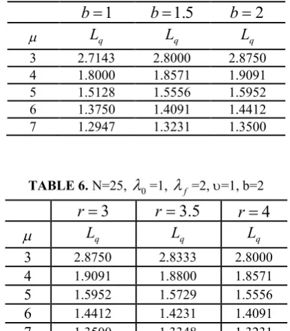
arrival rate (_f) whereas it decreases by increasing the service rates (). Figure 2 exhibits the mean queue length (L_q) by varying service rate (



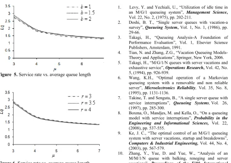
) and breakdown rate (b). It is seen that L_q decreases with the increase of service rate (), and L_q

increases with breakdown rate (b). Figure 3

demonstrates the mean queue length (L_q)

decreases with the increase of service rate () and repair rate (r).

When



s 0

For



_s 0

TABLE 4. N=25,



₀=1, =1, r=3, b=2

7







7.5



8

f Lq Lq Lq

2 1.3500 1.3171 1.2899

3 1.5147 1.4505 1.4000

4 1.8333 1.6912 1.5882

5 2.5909 2.2000 1.9524

6 5.37500 3.6316 2.8182

TABLE 5.N=25,



₀=1,



_f =2, =1, r=3

1

b



b



1.5

b



2

 Lq Lq Lq

3 2.7143 2.8000 2.8750

4 1.8000 1.8571 1.9091

5 1.5128 1.5556 1.5952

6 1.3750 1.4091 1.4412

7 1.2947 1.3231 1.3500

TABLE 6.N=25,



₀=1,



_f=2, =1, b=2

3

r



r



3.5

r



4

 Lq Lq Lq

3 2.8750 2.8333 2.8000

4 1.9091 1.8800 1.8571

5 1.5952 1.5729 1.5556

6 1.4412 1.4231 1.4091

7 1.3500 1.3348 1.3231

Figure 1. Fast arrival rate vs. average queue length

Figure 2. Service rate vs. average queue length

Figures 4, 5, 6 give the comparison of mean queue length (L_q) when no arrival during breakdown (i.e.

0 s

  ) with Figures 1, 2, 3 the mean queue length (L_q) when there may be arrivals during breakdown (i.e. s >0). This comparison shows that mean queue length (L_q) in latter figures increases or

decreases gradually than in former cases. When

0

s





,

5. DISCUSSION

By using partial generating function method we have obtained various performance measures for a single server, finite capacity queueing system with the provision of vacations and server breakdowns. The imposition of various arrival rates to the system may have the applicability in the real life queueing system in which arrival rates can be varied so as to reduce sufficient queue length. Proposed model may have potential application in the telecommunication system, computer communication systems, machining system, etc.

6. ACKNOWLEDGEMENT

Second author is thankful to both University Grant Commission (UGC) Nepal, for providing financial support and also to the School of Science, Kathmandu University (Nepal).

7. REFERENCES

1. Levy, Y. and Yechiali, U., “Utilization of idle time in an M/G/1 queueing system”, Management Science, Vol. 22, No. 2, (1975), pp. 202-211.

2. Doshi, B. T., “Single server queues with vacation-a survey”, Queueing System, Vol. 1, No. 1, (1986), pp. 29-66.

3. Takagi, H., “Queueing Analysis-A Foundation of Performance Evaluation”, Vol. 1, Elsevier Science Publishers, Amsterdam, 1991.

4. Tian, N. and Zhang, Z.G., “Vacation Queueing Models-Theory and Applications”, Springer, New York, 2006. 5. Takagi, H., “M/G/1/N queues with server vacations and

exhaustive service”, Operations Research,Vol. 42, No. 5, (1994), pp. 926-939.

6. Wang, K.H., “Optimal operation of a Markovian queueing system with a removable and non reliable server”, Microelectronics Reliability, Vol. 35, No. 8, (1995), pp. 1131-1136.

7. Takine, T. and Senguta, B., “A single server queue with service interruptions”, Queueing Systems,Vol. 26, (1997), pp. 285-300.

8. Boxma, O., Mandjes, M. and Kella, O., “On a queueing model with service interruptions”, Probability in the Engineering and Informational Sciences, Vol. 22, (2008), pp. 537-555.

9. Ke, J. C., “The optimal control of an M/G/1 queueing system with server vacations, startup and breakdowns”, Computers & Industrial Engineering,Vol. 44, No. 4, (2003), pp. 567-579.

10. Zhang, Y., Yue, D. and Yue, W., “Analysis of an M/M/1/N queue with balking, reneging and server vacations”, Proceedings of the Fifth International

Figure 4.Fast arrival rate vs. average queue length

Figure 5.Service rate vs. average queue length

Symposium,(2005), pp. 37-47.

11. Wang, K. H., Chan, M. C. and Ke, J.C., “Maximum entropy analysis of the Mx_{/M/1 queueing system with}

multiple vacations and server breakdowns”, Computers & Industrial Engineering,Vol. 52, No. 2, (2007), pp. 192-202.

12. Jain, M. and Agrawal, P. K., “Optimal policy for bulk queue with multiple types of server breakdown”, International Journal of Operational Research, Vol. 4, No. 1, (2009), pp. 35-54.

13. Ke, J. C. and Wang, K. H., “Analysis of operating characteristics for the heterogeneous batch arrival queue with server startup and breakdowns”, RAIRO Operations Research,Vol. 37, (2003), pp. 157-177. 14. Srivastava, V. and Jain, M., “Optimal N- policy for

single server Markovian queue with breakdown repair and state dependent arrival rate”, Journal of the Operations Research Society of India (OPSEARCH),

Vol. 36, No. 1, (1999), pp.75.

15. Hur, S. and Paik, S.J., “The effect of different arrival rates on the N-policy of M/G/1 with server setup, Applied Mathematical Modelling,Vol. 23, (1999), pp. 289-299.

16. Ke, J. C. and Pearn, W.L., “Optimal management policy for heterogeneous arrival queueing systems with server breakdowns and vacations”, Quality Technology and Quantitative management, Vol. 1 No. 1, (2004), pp. 149-162.

17. Gray, W. J., Wang, P. P. and Scott, M., “A vacation queueing model with service breakdowns”, Applied Mathematical Modeling,Vol. 24, (2000), pp. 391-400. 18. Gray, W. J., Wang, P.P. and Scott, M., “A queueing