Volume 2007, Article ID 85438,15pages doi:10.1155/2007/85438
Research Article
Underdetermined Blind Audio Source Separation Using
Modal Decomposition
Abdeldjalil A¨ıssa-El-Bey, Karim Abed-Meraim, and Yves Grenier
D´epartment TSI, ´Ecole Nationale Sup´erieure des T´el´ecommunications (ENST), 46 Rue Barrault, 75634 Paris Cedex 13, France
Received 1 July 2006; Revised 20 November 2006; Accepted 14 December 2006
Recommended by Patrick A. Naylor
This paper introduces new algorithms for the blind separation of audio sources using modal decomposition. Indeed, audio signals and, in particular, musical signals can be well approximated by a sum of damped sinusoidal (modal) components. Based on this representation, we propose a two-step approach consisting of a signal analysis (extraction of the modal components) followed by a signal synthesis (grouping of the components belonging to the same source) using vector clustering. For the signal analysis, two existing algorithms are considered and compared: namely the EMD (empirical mode decomposition) algorithm and a parametric estimation algorithm using ESPRIT technique. A major advantage of the proposed method resides in its validity for both instanta-neous and convolutive mixtures and its ability to separate more sources than sensors. Simulation results are given to compare and assess the performance of the proposed algorithms.
Copyright © 2007 Abdeldjalil A¨ıssa-El-Bey et al. This is an open access article distributed under the Creative Commons Attribution License, which permits unrestricted use, distribution, and reproduction in any medium, provided the original work is properly cited.
1. INTRODUCTION
The problem of blind source separation (BSS) consists of finding “independent” source signals from their observed mixtures without a priori knowledge on the actual mixing channels.
The source separation problem is of interest in various applications [1,2] such as the localization and tracking of targets using radars and sonars, separation of speakers (prob-lem known as “cocktail party”), detection and separation in multiple-access communication systems, independent com-ponent analysis of biomedical signals (EEG or ECG), multi-spectral astronomical imaging, geophysical data processing, and so forth [2].
This problem has been intensively studied in the litera-ture and many effective solutions have been proposed so far [1–3]. Nevertheless, the literature intended for the underde-termined case where the number of sources is larger than the number of sensors (observations) is relatively limited, and achieving the BSS in that context is one of the challenging problems in this field. Existing methods for the underdeter-mined BSS (UBSS) include the matching pursuit methods in [4,5], the separation methods for finite alphabet sources in [6,7], the probabilistic-based (using maximum a
0 0.2 0.4 0.6 0.8 1 Normalized frequency (πrad/sample)
100 150 200 250 300 350 400 450 500 550
Ti
m
e
Figure1: Time-frequency representation of a three-modal-compo-nent signal (using short-time Fourier transform).
Note that this modal representation of the sources is a particular case of signal sparsity often used to separate the sources in the underdetermined case [23]. Indeed, a signal given by a sum of sinusoids (or damped sinusoids) occupies only a small region in the time-frequency (TF) domain, that is, its TF representation is sparse. This is illustrated by Fig-ure1where we represent the time-frequency distribution of a three-modal-component signal.
The paper is organized as follows. Section2formulates the UBSS problem and introduces the assumptions necessary for the separation of audio sources using modal decomposi-tion. Section3proposes two MD-UBSS algorithms for in-stantaneous mixture case while Section4introduces a modi-fied version of MD-UBSS that relaxes the quasiorthogonality assumption of the source modal components. In Section5, we extend our MD-UBSS algorithm to the convolutive mix-ture case. Some discussions on the proposed methods are given in Section6. The performance of the above methods is numerically evaluated in Section7. The last section is for the conclusion and final remarks.
2. PROBLEM FORMULATION IN THE INSTANTANEOUS MIXTURE CASE
The blind source separation model assumes the existence of N independent signals s1(t),. . .,sN(t) and M observations x1(t),. . .,xM(t) that represent the mixtures. These mixtures
are supposed to be linear and instantaneous, that is,
xi(t)=
N
j=1
ai jsj(t), i=1,. . .,M. (1)
This can be represented compactly by the mixing equation
x(t)=As(t), (2)
wheres(t) def= [s1(t),. . .,sN(t)]T is anN×1 column vector
collecting the real-valued source signals, vectorx(t),
simi-larly, collects theMobserved signals, and theM×Nmixing matrixA def= [a1,. . .,aN] withai = [a1i,. . .,aMi]T contains the mixture coefficients.
Now, ifN > M, that is, there are more sources than sensors, we are in the underdetermined case, and BSS be-comes UBSS (U stands for underdetermined). By underde-terminacy, we cannot, from the set of equations in (2), alge-braically obtain a unique solution, because this system con-tains more variables (sources) than equations (sensors). In this case,Ais no longer left invertible, because it has more columns than rows. Consequently, due to the underdeter-mined representation, the above system of (2) cannot be solved completely even with the full knowledge of A, un-less we have some specific knowledge about the underlying sources.
Next, we will make some assumptions about the data model in (2), necessary for our method to achieve the UBSS.
Assumption 1. The column vectors ofAare pairwise linearly independent.
That is, for any index pair i = j ∈ N, whereN = {1,. . .,N}, vectorsai andaj are linearly independent. This assumption is necessary because if otherwise, we havea2 = αa1 for example, then the input/output relation (2) can be
reduced to
x(t)=a1,a3,. . .,aN
s1(t) +αs2(t),s3(t),. . .,sN(t) T
, (3)
and hence the separation ofs1(t) ands2(t) is inherently
im-possible. This assumption is used later (in the clustering step) to separate the source modal components using their spatial directions given by the column vectors ofA.
It is known that BSS is only possible up to some scaling and permutation [3]. We take the advantage of these indeter-minacies to further make the following assumption without loss of generality.
Assumption 2. The column vectors ofAare of unit norm.
That is,ai =1 for alli∈N, where the norm hereafter is given in the Frobenius sense.
As mentioned previously, solving the UBSS problem re-quires strong a priori assumptions on the source signals. In our case, signal sparsity is considered in terms of modal rep-resentation of the input signals as stated by the fundamental assumption below.
Assumption 3. The source signals are sum of modal compo-nents.
Indeed, we assume here that each source signalsi(t) is a sum oflimodal componentscij(t),j=1,. . .,li, that is,
si(t)= li
j=1
cij(t), t=0,. . .,T−1, (4)
Standard BSS techniques are based on the source pendence assumption. In the UBSS case, the source inde-pendence is often replaced by the disjointness of the sources. This means that there exists a transform domain where the source representation has disjoint or quasidisjoint supports. The quasidisjointness assumption of the sources translates in our case into the quasiorthogonality of the modal compo-nents.
Assumption 4. The sources are quasiorthogonal, in the sense that
cij|cj
i cj
ic j i
≈0, for (i,j)=(i,j), (5)
where
cij|c
j i
def=T−1 t=0
cij(t)c j i(t), cj
i 2
=cij|c j i
.
(6)
In the case of sinusoidal signals, the quasiorthogonality of the modal components is nothing else than the Fourier qua-siorthogonality of two sinusoidal components with distinct frequencies. This can be observed in the frequency domain through the disjointness of their supports. This property is also preserved by filtering, which does not affect the fre-quency support, and hence the quasiorthogonality assump-tion of the signals (this is used later when considering the convolutive case).
3. MD-UBSS ALGORITHM
Based on the previous model, we propose an approach in two steps consisting of the following.
(i) An analysis step
In this step, one applies an algorithm of modal decompo-sition to each sensor output in order to extract all the har-monic components from them. We compare for this modal components extraction two decomposition algorithms that are the EMD (empirical mode decomposition) algorithm in-troduced in [16,17] and a parametric algorithm which esti-mates the parameters of the modal components modeled as damped sinusoids.
(ii) A synthesis step
In this step, we group together the modal components corre-sponding to the same source in order to reconstitute the orig-inal signal. This is done by observing that all modal compo-nents of a given source signal “live” in the same spatial direc-tion. Therefore, the proposed clustering method is based on the component’s spatial direction evaluated by correlation of the extracted (component) signal with the observed antenna signal.
(1) Extraction of all harmonic components from each sensor by applying modal decomposition.
(2) Spatial direction estimation by (14) and vector clustering byk-means algorithm [24].
(3) Source estimation by grouping together the modal com-ponents corresponding to the same spatial direction. (4) Source grouping and source selection by (18).
Algorithm1: MD-UBSS algorithm in instantaneous mixture case using modal decomposition.
Note that, by this method, each sensor output leads to an estimate of the source signals. Therefore, we end up withM estimates for each source signal. As the quality of source sig-nal extraction depends strongly on the mixture coefficients, we propose a blind source selection procedure to choose the “best” of theMestimates. This algorithm is summarized in Algorithm1.
3.1. Modal component estimation
3.1.1. Signal analysis using EMD
A new nonlinear technique, referred to asempirical mode de-composition(EMD), has recently been introduced by Huang et al. for representing nonstationary signals as sum of zero-mean AM-FM components [16]. The starting point of the EMD is to consider oscillations in signals at a very local level. Given a signalz(t), the EMD algorithm can be summarized as follows [17]:
(1) identify all extrema ofz(t). This is done by the algo-rithm in [25];
(2) interpolate between minima (resp., maxima), ending up with some envelopeemin(t) (resp.,emax(t)). Several
interpolation techniques can be used. In our simula-tion, we have used a spline interpolation as in [25]; (3) compute the meanm(t)=(emin(t) +emax(t))/2;
(4) extract the detaild(t)=z(t)−m(t);
(5) iterate on the residual1m(t) untilm(t)=0 (in
prac-tice, we stop the algorithm whenm(t) ≤, where is a given threshold value).
By applying the EMD algorithm to theith mixture signalxi which is written asxi(t)=N
j=1ai jsj(t)= N
j=1 lj
k=1ai jckj(t), one obtains estimatesckj(t) of componentsckj(t) (up to the scalar constantai j).
3.1.2. Parametric signal analysis
In this section, we present an alternative solution for signal analysis. For that, we represent the source signal as sum of
damped sinusoids:
si(t)= e l
i
j=1 αij
zij
t
, (7)
corresponding to
cij(t)= e
αij
zij t
, (8)
where αij = β j ieθ
j
i represents the complex amplitude and
zij=ed
j
i+jωijis thejth pole of the sourcesi, wheredj
i is the neg-ative damping factor andωijis the angular frequency.e(·) represents the real part of a complex entity. We denote byLtot
the total number of modal components, that is,Ltot= N
i=1li.
For the extraction of the modal components, we pro-pose to use the ESPRIT (estimation of signal parameters via rotational invariance technique) algorithm that estimates the poles of the signals by exploiting the row-shifting in-variance property of theD×(T−D) data Hankel matrix [H(xk)]n1n2
def=
xk(n1+n2),Dbeing a window parameter
cho-sen in the rangeT/3≤D≤2T/3.
More precisely, we use Kung’s algorithm given in [26] that can be summarized in the following steps:
(1) form the data Hankel matrixH(xk);
(2) estimate the 2Ltot-dimensional signal subspace U(Ltot) = [u
1,. . .,u2Ltot] ofH(xk) by means of the SVD of
H(xk) (u1,. . .,u2Ltot are the principal left singular eigenvec-tors ofH(xk));
(3) solve (in the least-squares sense) the shift invariance equation
U(Ltot)
↓ Ψ=U(↑Ltot)⇐⇒Ψ=U↓(Ltot)#U(↑Ltot), (9)
whereΨ=ΦΔΦ−1,Φbeing a nonsingular 2L
tot×2Ltot
ma-trix, andΔ=diag(z1
1,z1∗1 ,. . .,z1l1,zl11∗,. . .,zNlN,zNlN∗). (·)∗ rep-resents the complex conjugation, (·)#denotes the
pseudoin-version operation, and arrows↓and↑denote, respectively, the last and the first row-deleting operator;
(4) estimate the poles as the eigenvalues of matrixΨ; (5) estimate the complex amplitudes by solving the least-squares fitting criterion
min αk
xk−Zαk2⇐⇒αk=Z#xk, (10)
wherexk=[xk(0),. . .,xk(T−1)]T is the observation vector,
Zis a Vandermonde matrix constructed from the estimated poles, that is,
Z=z1
1,z1∗1 ,. . .,zl11,z1l1∗,. . .,zlNN,zlNN∗
, (11)
withzij =[1,zij, (z j
i)2,. . ., (z j
i)T−1]T, andαk is the vector of complex amplitudes, that is,
αk= 1 2
ak1α11,ak1α1∗1 ,. . .,ak1αl11∗,. . .,akNαlNN∗ T
. (12)
ai
aj
Figure2: Data clustering illustration, where we represent the dif-ferent estimatesaijand their centroids.
3.2. Clustering and source estimation
3.2.1. Signal synthesis using vector clustering
For the synthesis of the source signals, one observes that thanks to the quasiorthogonality assumption, one has
x|cij cj
i 2
def= 1
cj i
2 ⎡ ⎢ ⎢ ⎢ ⎣
x1|cij
.. .
xM |cij
⎤ ⎥ ⎥ ⎥
⎦≈ai, (13)
whereairepresents theith column vector ofA. We can, then, associate each component ckj to a spatial direction (vector column ofA) that is estimated by
akj =
x|ck j
ck j
2 . (14)
Vectorakj would be equal approximately toai (up to a scalar constant) ifckj is an estimate of a modal component of sourcei. Hence, two components of a same source signal are associated to colinear spatial direction of to the same col-umn vector ofA. Therefore, we propose to gather these com-ponents by clustering their directional vectors intoNclasses (see Figure2). For that, we compute first the normalized vec-tors
akj=a
k je−jψ
k j
akj , (15)
whereψk
j is the phase argument of the first entry ofakj(this is to force the first entry to be real positive). Then, these vectors are clustered byk-means algorithm [24] that can be summa-rized in the following steps.
(1) PlaceNpoints into the space represented by the vec-tors that are being clustered. These points represent initial group centroids. One popular way to start is to randomly chooseNvectors among the set of vectors to be clustered.
of theNclusters, one assigns the vectorakjto the cluster i0that satisfies
i0=arg min i
ak
j−yi. (16)
(3) When all vectors have been assigned, recalculate the positions of theNcentroids in the following way: for each cluster, the new centroid’s vector is calculated as the mean value of the cluster’s vectors.
(4) Repeat steps 2 and 3 until the centroids no longer move. This produces a separation of the vectors into Ngroups. In practice, in order to increase the conver-gence rate, one can also use a threshold value and stop the algorithm when the difference between the new and old centroid values is smaller than this threshold for allNclusters.
Finally, one will be able to rebuild the initial sources up to a constant by adding the various components within a same class, that is,
si(t)=
Ci
cij(t), (17)
whereCirepresents theith cluster.
3.2.2. Source grouping and selection
Let us notice that by applying the approach described previously (analysis plus synthesis) to all antenna outputs x1(t),. . .,xM(t), we obtainM estimates of each source
sig-nal. The estimation quality of a given source signal varies significantly from one sensor to another. Indeed, it depends strongly on the matrix coefficients and, in particular, on the signal-to-interference ratio (SIR) of the desired source. Con-sequently, we propose a blind selection method to choose a “good” estimate among theMwe have for each source signal. For that, we need first to pair the source estimates together. This is done by associating each source signal extracted from the first sensor to the (M−1) signals extracted from the (M−1) other sensors that are maximally correlated with it. The correlation factor of two signalss1ands2is evaluated by
|s1|s2|/s1s2.
Once the source grouping is achieved, we propose to se-lect the source estimate of maximal energy, that is,
si(t)=arg max sij(t)
Eij=
T−1
t=0 s j i(t)
2
, j=1,. . .,M
, (18)
where Eij represents the energy of the ith source extracted from thejth sensorsij(t). One can consider other methods of selection (based, e.g., on the dispersion around the centroid) or instead, a diversity combining technique for the different source estimates. However, the source estimates are very dis-similarly in quality, and hence we have observed in our simu-lations that the energy-based selection, even though not op-timal, provides the best results in terms of source estimation error.
3.3. Case of common modal components
We consider here the case where a given componentckj(t) as-sociated with the pole zkj can be shared by several sources. This is the case, for example, for certain musical signals such as those treated in [27]. To simplify, we suppose that a com-ponent belongs to at most two sources. Thus, let us sup-pose that the sinusoidal component (zk
j)t is present in the sourcessj1(t) andsj2(t) with the amplitudesαj1andαj2, re-spectively (i.e., one modal component of sourcesj1(resp.,sj2) ise(αj1(zkj)t) (resp.,e(αj2(zkj)t))). It follows that the spa-tial direction associated with this component is a linear com-bination of the column vectorsaj1andaj2. More precisely, we have
akj= 1
zkj2
⎡ ⎢ ⎢ ⎢ ⎣
x1Tzkj .. .
xTMzkj
⎤ ⎥ ⎥ ⎥
⎦≈αj1aj1+αj2aj2. (19)
It is now a question of finding the indices j1 and j2of the
two sources associated with this component, as well as the amplitudesαj1andαj2. With this intention, one proposes an approach based on subspace projection. Let us assume that M >2 and that matrixAis known and satisfies the condition that any triplet of its column vectors is linearly independent. Consequently, we have
P⊥ Aa
k
j=0, (20) if and only ifA = [aj1 aj2],A being a matrix formed by a pair of column vectors ofAandP⊥
Arepresents the matrix of
orthogonal projection on the orthogonal range space ofA, that is,
P⊥
A=I−AA
HA−1AH, (21)
whereIis the identity matrix and (·)Hdenotes the transpose conjugate. In practice, by taking into account the noise, one detects the columns j1andj2by minimizing
j1,j2
=arg min
(l,m)
P⊥ Aa
k j|A=
al am . (22)
OnceAfound, one estimates the weightingsαj1andαj2by
αj1 αj2
=A#ak
j. (23)
In this paper, we treated all the components as being asso-ciated to two source signals. If ever a component is present only in one source, one of the two coefficients estimated in (23) should be zero or close to zero.
In what precedes, the mixing matrixAis supposed to be known. This means that it has to be estimated before apply-ing a subspace projection. This is performed here by clus-tering all the spatial direction vectors in (14) as for the pre-vious MD-UBSS algorithm. Then, theith column vector of
4. MODIFIED MD-UBSS ALGORITHM
We propose here to improve the previous algorithm with respect to the computational cost and the estimation accu-racy when Assumption4is poorly satisfied.2 First, in order
to avoid repeated estimation of modal components for each sensor output, we use all the observed data to estimate (only once) the poles of the source signals. Hence, we apply the ES-PRIT technique on the averaged data covariance matrixH(x) define by
H(x)=
M
i=1
HxiHxiH (24)
and we apply steps 1 to 4 of Kung’s algorithm described in Section 3.1.2 to obtain all the poles zij, i = 1,. . .,N, j=1,. . .,li. In this way, we reduce significantly the compu-tational cost and avoid the problem of “best source estimate” selection of the previous algorithm.
Now, to relax Assumption 4, we can rewrite the data model as
Γz(t)=x(t), (25)
where Γ def= [γ1
1,γ11,. . .,γ lN
N,γlNN], γ j i = β
j iejφ
j ibj
i and γ j i = βije−jφ
j ibj
i, whereb j
i is a unit norm vector representing the spatial direction of the ith component (i.e.,bij = ak if the component (zij)tbelongs to thekth source signal) andz(t)
def
=
[(z1
1)t, (z1∗1 )t,. . ., (zNlN)t, (zlNN∗)t]T.
The estimation ofΓusing the least-squares fitting crite-rion leads to
min
Γ X−ΓZ
2⇐⇒Γ=XZ#, (26)
whereX=[x(0),. . .,x(T−1)] andZ=[z(0),. . .,z(T−1)]. After estimatingΓ, we estimate the phase of each pole as
φij=
argγijHγij
2 . (27)
The spatial direction of each modal component is estimated by
aij=γj ie−jφ
j
i +γj
iejφ
j
i =2βj
ib j
i. (28) Finally, we group together these components by clustering the vectorsaij intoN classes. After clustering, we obtainN classes withNunit-norm centroidsa1,. . .,aNcorresponding to the estimates of the column vectors of the mixing matrix
A. If the polezij belongs to thekth class, then according to (28), its amplitude can be estimated by
βij=
aTkaij
2 . (29)
2This is the case when the modal components are closely spaced or for modal components with strong damping factors.
One will be able to rebuild the initial sources up to a constant by adding the various modal components within a same class
Ckas follows:
sk(t)= e
Ck
βijejφ
j izj
i t
. (30)
Note that one can also assign each component to two (or more) source signals as in Section3.3by using (20)–(23).
5. GENERALIZATION TO THE CONVOLUTIVE CASE
The instantaneous mixture model is, unfortunately, not valid in real-life applications where multipath propagation with large channel delay spread occurs, in which case convolutive mixtures are considered.
Blind separation of convolutive mixtures and multi-channel deconvolution has received wide attention in vari-ous fields such as biomedical signal analysis and processing (EEG, MEG, ECG), speech enhancement, geophysical data processing, and data mining [2].
In particular, acoustic applications are considered in sit-uations where signals, from several microphones in a sound field produced by several speakers (the so-called cocktail-party problem) or from several acoustic transducers in an underwater sound field produced by engine noises of several ships (sonar problem), need to be processed.
In this case, the signal can be modeled by the following equation:
x(t)=
K
k=0
H(k)s(t−k) +w(t), (31)
whereH(k) areM×N matrices for k ∈ [0,K] represent-ing the impulse response coefficients of the channel. We con-sider in this paper the underdetermined case (M < N). The sources are assumed, as in the instantaneous mixture case, to be decomposable in a sum of damped sinusoids satisfy-ing approximately the quasiorthogonality Assumption4. The channel satisfies the following diversity assumption.
Assumption 5. The channel is such that each column vector of
H(z)def=
K
k=0
H(k)z−kdef=h
1(z),. . .,hN(z)
(32)
is irreducible, that is, the entries ofhi(z) denoted byhi j(z), j =1,. . .,M, have no common zero for alli. Moreover, any two column vectors ofH(z) form an irreducible polynomial matrixH(z), that is, rank (H(z))=2 for allz.
0 1 2 3 4 5 6 −1
0 1
s1
0 1 2 3 4 5 6
−1 0 1
s2
0 1 2 3 4 5 6
−1 0 1
s3
0 1 2 3 4 5 6
Time (s) −1
0 1
s4
Figure3: Time representation of 4 audio sources: this representa-tion illustrates the audio signal sparsity (i.e., there exist time inter-vals where only one source is present).
corresponding to a polezijof sourcesiwith the observed sig-nalx(t) leads to an estimate of vectorhi(zij). Therefore, two components of respective poleszijandzki of the same source signalsiwill produce spatial directionshi(zij) andhi(zik) that are not colinear. Consequently, the clustering method used for the instantaneous mixture case cannot be applied in this context of convolutive mixtures.
In order to solve this problem, it is necessary to iden-tify first the impulse response of the channels. This problem in overdetermined case is very difficult and becomes almost impossible in the underdetermined case without side infor-mation on the considered sources. In this work and simi-lar to [28], we exploit the sparseness property of the audio sources by assuming that from time to time, only one source is present. In other words, we consider the following assump-tion.
Assumption 6. There exist, periodically, time intervals where only one source is present in the mixture. This occurs for all source signals of the considered mixtures (see Figure3).
To detect these time intervals, we propose to use infor-mation criterion tests for the estiinfor-mation of the number of sources present in the signal (see Section5.1for more de-tails). An alternative solution would be to use the “frame se-lection” technique in [29] that exploits the structure of the spectral density function of the observations. The algorithm in convolutive mixture case is summarized in Algorithm2.
5.1. Channel estimation
Based on Assumption 6, we propose here to apply SIMO-(single-input-multiple-output-) based techniques to blindly estimate the channel impulse response. Regarding the
prob-(1) Channel estimation; AIC criterion [30] to detect the number of sources and application of blind identification algorithm [31,32] to estimate the channel impulse response.
(2) Extraction of all harmonic components from each sensor by applying parametric estimation algorithm (ESPRIT technique).
(3) Spatial direction estimation by (44).
(4) Source estimation by grouping together, using (45), the modal components corresponding to the same source (channel).
(5) Source grouping and source selection by (18).
Algorithm2: MD-UBSS algorithm in convolutive mixture case us-ing modal decomposition.
lem at hand, we have to solve 3 different problems: first, we have to select time intervals where only one source signal is effectively present; then, for each selected time interval one should apply an appropriate blind SIMO identification tech-nique to estimate the channel parameters; finally, in the way we proceed, the same channel may be estimated several times and hence one has to group together (cluster) the channel es-timates intoNclasses corresponding to theNsource chan-nels.
5.1.1. Source number estimation
Let define the spatiotemporal vector
xd(t)=
xT(t),. . .,xT(t−d+ 1)T = N
k=1
Hksk(t) +wd(t),
(33)
whereHkare block-Sylvester matrices of sizedM×(d+K) andsk(t)def=[sk(t),. . .,sk(t−K−d+ 1)]T.dis a chosen pro-cessing window size. Under the no-common zeros assump-tion and for large window sizes (see [30] for more details), matricesHkare full column rank.
Hence, in the noiseless case, the rank of the data co-variance matrix R def= E[xd(t)xHd(t)] is equal to min(p(d+ K),dM), where p is the number of sources present in the considered time interval over which the covariance matrix is estimated. In particular, forp=1, one has the minimum rank value equal to (d+K).
Therefore, our approach consists in estimating the rank of the sample averaged covariance matrixRover several time slots (intervals) and selecting those corresponding to the smallest rank valuer =d+K.
1 2 3 Estimated number of sources 0
20 40 60 80 100 120 140
N
u
mber
of
time
int
er
vals
Figure4: Histogram representing the number of time intervals for each estimated number of sources for 4 audio sources and 3 sensors in convolutive mixture case.
The estimation of the rank value is done here by Akaike’s information criterion (AIC) [30] according to
r =arg min k
−2 log
Md
i=k+1λ1i/(Md−k)
1/(Md−k) Mdi=k+1 λi
(Md−k)Ts
+ 2k(2Md−k)
,
(34)
whereλ1 ≥ · · · ≥ λMdrepresent the eigenvalues ofR and Tsis the time slot size. Note that it is not necessary at this stage to know exactly the channel degreeKas long asd > K (i.e., an overestimation of the channel degree is sufficient) in which case the presence of one source signal is characterized by
d < r <2d. (35)
Figure4illustrates the effectiveness of the proposed method where a recording of 6 seconds ofM =3 convolutive mix-tures ofN=4 sources is considered. The sampling frequency is 8 KHz and the time slot size isTs=200 samples. The fil-ter coefficients are chosen randomly and the channel order isK = 6. One can observe that the case p =1 (one source signal) occurs approximatively 10% of the time in the con-sidered context.
5.1.2. Blind channel identification
To perform the blind channel identification, we have used in this paper the cross-relation (CR) technique described in [31,32]. Consider a time interval where we have only the sourcesipresent. In this case, we can consider a SIMO system
ofMoutputs given by
x(t)=
K
k=0
hi(k)si(t−k) +w(t), (36)
wherehi(k)=[hi1(k)· · ·hiM(k)]T,k=0,. . .,K. From (36),
the noise-free outputsxj(k), 1≤j≤M, are given by xj(k)=hi j(k)∗si(k), 1≤ j≤M, (37)
where “∗” denotes the convolution. Using commutativity of convolution, it follows that
hil(k)∗xj(k)=hi j(k)∗xl(k), 1≤j < l≤M. (38) This is a linear equation satisfied by every pair of channels. It was shown that reciprocally the previousM(M−1)/2 cross-relations characterize uniquely the channel parameters. We have the following theorem [31].
Theorem 1. Under the no-common zeros assumption, the set of cross-relations (in the noise free case):
xl(k)∗hj(k)−xj(k)∗hl(k)=0, 1≤l < j≤M, (39)
whereh(z)=[h1(z)· · ·hM(z)]Tis anM×1polynomial
vec-tor of degreeK, is satisfied if and only ifh(z)=αhi(z)for a
given scalar constantα.
By collecting all possible pairs ofM channels, one can easily establish a set of linear equations. In matrix form, this set of equations can be expressed as
XMhi=0, (40)
wherehi def= [hi1(0)· · ·hi1(K),. . .,hiM(0)· · ·hiM(K)]T and XMis defined by
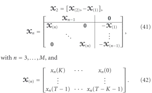
X2=
X(2),−X(1)
,
Xn= ⎡ ⎢ ⎢ ⎢ ⎢ ⎣
Xn−1 0
X(n) 0 −X(1)
. .. ...
0 X(n) −X(n−1) ⎤ ⎥ ⎥ ⎥ ⎥ ⎦,
(41)
withn=3,. . .,M, and
X(n)= ⎡ ⎢ ⎢ ⎣
xn(K) · · · xn(0) ..
. ...
xn(T−1) · · · xn(T−K−1) ⎤ ⎥ ⎥
⎦. (42)
In the presence of noise, (40) can be naturally solved in the least-squares (LS) sense according to
hi=arg min
h=1h
HXH
MXMh, (43)
which solution is given by the least eigenvector of matrix
Remark 1. We have presented here a basic version of the CR method. In [33], an improved version of the method (in-troduced in the adaptive scheme) is proposed exploiting the quasisparse nature of acoustic impulse responses.
5.1.3. Clustering of channel vector estimates
The first step of our channel estimation method consists in detecting the time slots where only one single source signal is “effectively” present. However, the same source signalsimay be present in several time intervals (see Figures3and4) lead-ing to several estimates of the same channel vectorhi.
We end up, finally, with several estimates of each source channel that we need to group together intoNclasses. This is done by clustering the estimated vectors usingk-means algo-rithm. Theith channel estimate is evaluated as the centroid of theith class.
5.2. Component grouping and source estimation
For the synthesis of the source signals, one observes that the quasiorthogonality assumption leads to
hij=
x|cij
cij
2 ∝hi
zij
, (44)
wherezij =ed
j
i+jωij is the pole of the component cj
i, that is, cij(t)= e{α
j i(z
j
i)t}. Therefore, we propose to gather these components by minimizing the criterion3:
cij∈Ci⇐⇒i=arg min l
min
α h j i −αhl
zij
2
, (45)
i=arg min l
hij2−hHl
zij h j i
2 hl
zij 2
, (46)
wherehlis thelth column ofHestimated in Section5.1and
hl(zkj) is computed by
hl
zij
=
K
k=0 hl(k)
zij
−k
. (47)
One will be able to rebuild the initial sources up to a constant by adding the various components within a same class using (17).
Similar to the instantaneous mixture case, one modal component can be assigned to two or more source signals, which relaxes the quasiorthogonality assumption and im-proves the estimation accuracy at moderate and high SNRs (see Figure9).
3We minimize over the scalarαbecause of the inherent indeterminacy of the blind channel identification, that is,hi(z) is estimated up to a scalar constant as shown by Theorem1.
6. DISCUSSION
We provide here some comments to get more insight onto the proposed separation method.
(i) Overdetermined case
In that case, one is able to separate the sources by left inver-sion of matrixA(or matrixHin the convolutive case). The latter can be estimated from the centroids of theN clusters (i.e., the centroid of theith cluster represents the estimate of theith column ofA).
(ii) Estimation of the number of sources
This is a difficult and challenging task in the underdeter-mined case. Few approaches exist based on multidimensional tensor decomposition [34] or based on the clustering with joint estimation of the number of classes [24]. However, these methods are very sensitive to noise, to the source am-plitude dynamic, and to the conditioning of matrixA. In this paper, we assumed that the number of sources is known (or correctly estimated).
(iii) Number of modal components
In the parametric approach, we have to choose the number of modal componentsLtot needed to well-approximate the
audio signal. Indeed, small values ofLtotlead to poor signal
representation while large values ofLtotincrease the
compu-tational cost. In fact,Ltotdepends on the “signal complexity,”
and in general musical signals require less components (for a good modeling) than speech signals [35]. In Section7, we illustrate the effect of the value ofLtoton the separation
qual-ity.
(iv) Hybrid separation approach
It is most probable that the separation quality can be further improved using signal analysis in conjunction with spatial fil-tering or interference cancelation as in [28]. Indeed, it has been observed that the separation quality depends strongly on the mixture coefficients. Spatial filtering can be used to improve the SIR for a desired source signal, and consequently its extraction quality. This will be the focus of a future work.
(v) SIMO versus MIMO channel estimation
0 5 10 ×103 −1
−0.5 0 0.5 1
0 5 10
×103 −1
−0.5 0 0.5 1
0 5 10
×103 −1
−0.5 0 0.5 1
0 5 10
×103 −1
−0.5 0 0.5 1
0 5 10
×103 −1
−0.5 0 0.5 1
0 5 10
×103 −1
−0.5 0 0.5 1 1.5
0 5 10
×103 −1
−0.5 0 0.5 1
0 5 10
×103 −1
−0.5 0 0.5 1
0 5 10
×103 −1
−0.5 0 0.5 1
0 5 10
×103 −1
−0.5 0 0.5 1
0 5 10
×103 −1
−0.5 0 0.5 1
0 5 10
×103 −0.2
−0.1 0 0.1 0.2
Figure5: Blind source separation example for 4 audio sources and 3 sensors in instantaneous mixture case: the upper line represents the original source signals, the second line represents the source estimation by pseudoinversion of mixing matrixAassumed exactly known and the bottom one represents estimates of sources by our algorithm using EMD.
(vi) Noiseless case
In the noiseless case (with perfect modelization of the sources as sums of damped sinusoids), the estimation of the modal components using ESPRIT would be perfect. This would lead to perfect (exact) estimation of the mixing matrix column vectors using least-squares filtering, and hence perfect clus-tering and source restoration.
7. SIMULATION RESULTS
We present here some simulation results to illustrate the per-formance of our blind separation algorithms. For that, we consider first an instantaneous mixture with a uniform linear array ofM=3 sensors receiving the signals fromN=4 au-dio sources (except for the third experiment whereNvaries in the range [2· · ·6]). The angle of arrivals (AOAs) of the sources is chosen randomly.4In the convolutive mixture case,
the filter coefficients are chosen randomly and the channel order isK=6. The sample size is set toT =10000 samples (the signals are sampled at a rate of 8 KHz). The observed signals are corrupted by an additive white noise of covari-anceσ2I(σ2being the noise power). The separation quality
is measured by the normalized mean-squares estimation er-rors (NMSEs) of the sources evaluated overNr=100 Monte Carlo runs. The plots represent the averaged NMSE over the
4This is used here just for the simulation to generate the mixture matrix
A. We do not consider a parametric model using sources AOAs in our separation algorithm.
Nsources:
NMSEidef= 1 Nr
Nr
r=1
min α
α si,r−si2 si2
,
NMSEi= 1 Nr
Nr
r=1
1−
!
si,rsTi
si,rsi "2
,
NMSE= 1
N N
i=1
NMSEi,
(48)
wheresidef=[si(0),. . .,si(T−1)],si,r(defined similarly) is the rth estimate of sourcesi, andαis a scalar factor that compen-sates for the scale indeterminacy of the BSS problem.
In Figure5, we present a simulation example withN=4 audio sources. The upper line represents the original source signals, the second line represents the source estimation by pseudoinversion of mixing matrixAassumed exactly known, and the bottom one represents estimates of the sources by our algorithm.
In Figure6, we compare the separation performance ob-tained by our algorithm using EMD and the parametric tech-nique with L = 30 modal components per source signal (Ltot = NL). As a reference, we plot also the NMSE
ob-tained by pseudoinversion of matrix A[36] (assumed ex-actly known). It is observed that both EMD and parametric-based separation provide better results than those obtained by pseudoinversion of the exact mixing matrix.
0 5 10 15 20 25 30 SNR (dB)
−10 −9 −8 −7 −6 −5 −4 −3 −2 −1
NMSE
(dB)
EMD
ParametricL=30 Pseudoinversion
Figure6: NMSE versus SNR for 4 audio sources and 3 sensors in instantaneous mixture case: comparison of the performance of our algorithm (EMD and ESPRIT) with those given by the pseudoin-version of mixing matrixA(assumed exactly known).
10 15 20 25 30 35 40
Number of components −9.5
−9 −8.5 −8 −7.5 −7 −6.5
NMSE
(dB)
Parametric SNR=30 dB Parametric SNR=10 dB
Figure7: NMSE versusLfor 4 audio sources and 3 sensors in in-stantaneous mixture case: comparison of the performance of our algorithm (ESPRIT) forL varying in the range [10,. . ., 40] with SNR=10 dB and SNR=30 dB.
In other words, there exists an optimal choice ofLthat de-pends on the signal type.
In Figure8, we compare the separation performance loss that we have when the number of sources increases from 2 to 6 in the noiseless case. ForN = 2 andN = 3 (overde-termined case), we estimate the sources by left inversion of the estimate of matrixA. In the underdetermined case, the EMD and parametric-based algorithms present similar
per-2 2.5 3 3.5 4 4.5 5 5.5 6 Number of sources
−45 −40 −35 −30 −25 −20 −15 −10 −5 0
NMSE
(dB)
EMD
ParametricL=30
Figure8: NMSE versusN for 3 sensors in instantaneous mixture case: comparison of the performance of our algorithm (EMD and ESPRIT) forN∈[2,. . ., 6].
0 5 10 15 20 25 30 35 40
SNR (dB) −11
−10 −9 −8 −7 −6 −5 −4 −3
NMSE
(dB)
Parametric with subspace projection Parametric
Figure9: NMSE versus SNR for 4 audio sources and 3 sensors in instantaneous mixture case: comparison of the performance of our algorithm (EMD) and the same algorithm with subspace projec-tion.
formance. However, the latter method is better in the overde-termined case.
0 5 10 15 20 25 30 SNR (dB)
−10 −9 −8 −7 −6 −5 −4
NMSE
(dB)
Modified MD-UBSS
MD-UBSS with energy-based selection MD-UBSS with optimal selection
Figure10: NMSE versus SNR for 4 audio sources and 3 sensors: comparison of the performance of MD-UBSS algorithms with and without quasiorthogonality assumption.
to only one source signal, (23) would provide a nonzero am-plitude coefficient for the second source due to noise effect which explains the observed degradation.
In Figure10, we compare the separation performance ob-tained by our UBSS algorithm and the modified MD-UBSS algorithm. We observe a performance gain in favor of the modified MD-UBSS mainly due to the fact that it does not rely on the quasiorthogonality assumption. This plot also highlights the problem of “best source estimate” selec-tion related to the MD-UBSS as we observe a performance loss between the results given by the proposed energy-based selection procedure and the optimal5 one using the exact
source signals.
Figure11 illustrates the estimation performance of the mixing matrixAusing proposed clustering method. The ob-served good estimation performance translates the fact that most modal components belong “effectively” to one single source signal.
In Figure 12, we present the performance of channel identification obtained by using SIMO identification algo-rithm (in this case, we choose only the time intervals where only one source is present using AIC criterion) with SIMO and MIMO identification algorithms (in this case, we choose the time intervals where we are in the overdetermined case; i.e., wherep =1 or p=2). It is observed that SIMO-based identification provides better results than those obtained by SIMO and MIMO identification algorithms.
5Clearly, the optimal selection procedure is introduced here just for per-formance comparison and not as an alternative selection method since it relies on the exact source signals that are unavailable in our context.
0 5 10 15 20 25 30 35 40
SNR (dB) −25
−20 −15 −10
NMSE
(dB)
Figure 11: Mixing matrix estimation: NMSE versus SNR for 4 speech sources and 3 sensors in instantaneous mixture case.
10 15 20 25 30
SNR (dB) −30
−25 −20 −15 −10 −5
NMSE
(dB)
SIMO
SIMO and MIMO
Figure12: NMSE versus SNR for 4 audio sources and 3 sensors in convolutive mixture case: comparison of the performance of identi-fication algorithm using only SIMO system and the algorithm using SIMO and MIMO systems.
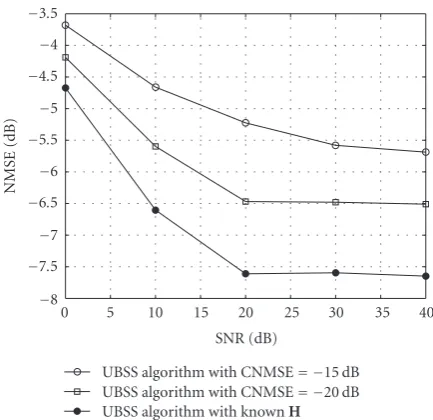
The plots in Figure 13 present the separation perfor-mance in convolutive mixture case when using the exact channel impulse responseHcompared to that obtained with an approximate channelH =H+δH, where the entries of δHare i.i.d. Gaussian distributed. This is done for different values of channel normalized mean-squares error (CNMSE) defined by
CNMSE=10 logH−H
2
0 5 10 15 20 25 30 35 40 SNR (dB)
−8 −7.5 −7 −6.5 −6 −5.5 −5 −4.5 −4 −3.5
NMSE
(dB)
UBSS algorithm with CNMSE= −15 dB UBSS algorithm with CNMSE= −20 dB UBSS algorithm with knownH
Figure13: NMSE versus SNR for 4 audio sources and 3 sensors in convolutive mixture case: comparison, for the MD-UBSS algorithm in convolutive mixture case, when the channel responseHis known or disturbed by Gaussian noise for different values of CNMSE.
0 5 10 15 20 25 30 35 40
SNR (dB) −8
−7 −6 −5 −4 −3 −2
NMSE
(dB)
UBSS algorithm
UBSS algorithm with knownH
Figure14: NMSE versus SNR for 4 audio sources and 3 sensors in convolutive mixture case: comparison, for the MD-UBSS algorithm in convolutive mixture case, when the channel responseHis known or estimated using the CR technique.
Clearly, the separation quality depends strongly on the qual-ity of channel estimation.
In Figure 14, we present the separation performance when using the exact channel responseHcompared to that obtained with the proposed estimate H using SIMO ap-proach. For SNRs larger than 20 dB, the channel estimation is good enough for the proposed method to achieve almost
the same performance as if the channel is exactly known. Surprisingly, at SNR = 20 dB, the channel estimate NMSE is approximately equal to−18 dB (see Figure 12), an error level corresponding to a nonnegligible degradation shown in Figure13. This seemingly contradiction comes from the fact that in the experiment of Figure13, the channel is disturbed “artificially” using spatially white Gaussian noise, while the real channel estimation error is spatially colored (see, e.g., [37] where explicit expression of the asymptotic channel co-variance error is given) which seems to be favorable to our separation method.
8. CONCLUSION
This paper introduces a new blind separation method for audio-type sources using modal decomposition. The pro-posed method can separate more sources than sensors and provides, in that case, a better separation quality than the one obtained by pseudoinversion of the mixture matrix (even if the latter is known exactly) in the instantaneous mixture case. The separation method proceeds in two steps: an anal-ysis step where all modal components are estimated followed by a synthesis step to group (cluster) together the modal components and reconstruct the source signals. For the sig-nal asig-nalysis step, two algorithms are used and compared based, respectively, on the EMD and on the ESPRIT tech-niques. A modified MD-UBSS as well as a subspace projec-tion approach are also proposed to relax the “quasiorthog-onality” assumption and allow the source signals to share common modal components, respectively. This approach leads to a performance improvement of the separation qual-ity. For the convolutive mixture case, we propose to use again modal decomposition based on ESPRIT technique, but the signal synthesis is more complex and requires the prior iden-tification of the channel impulse response, which is done here using the sparsity of the audio sources.
ACKNOWLEDGMENT
Part of this work has been published in conferences [38,39].
REFERENCES
[1] A. K. Nandi, Ed.,Blind Estimation Using Higher-Order Statis-tics, Kluwer Academic, Boston, Mass, USA, 1999.
[2] A. Cichocki and S. Amari,Adaptive Blind Signal and Image Processing, John Wiley & Sons, Chichester, UK, 2003. [3] J.-F. Cardoso, “Blind signal separation: statistical principles,”
Proceedings of the IEEE, vol. 86, no. 10, pp. 2009–2025, 1998. [4] P. Sugden and N. Canagarajah, “Underdetermined noisy blind
separation using dual matching pursuits,” in Proceedings of IEEE International Conference on Acoustics, Speech and Signal Processing (ICASSP ’04), vol. 5, pp. 557–560, Montreal, Que, Canada, May 2004.
[5] P. Sugden and N. Canagarajah, “Underdetermined blind sep-aration using learned basis function sets,”Electronics Letters, vol. 39, no. 1, pp. 158–160, 2003.
[7] A. Belouchrani and J. F. Cardoso, “A maximum likelihood source separation for discrete sources,” inProceedings of the 7th European Signal Processing Conference (EUSIPCO ’94), vol. 2, pp. 768–771, Scotland, UK, September 1994.
[8] J. M. Peterson and S. Kadambe, “A probabilistic approach for blind source separation of underdetermined convolutive mixtures,” inProceedings of IEEE International Conference on Acoustics, Speech and Signal Processing (ICASSP ’03), vol. 6, pp. 581–584, Hong Kong, April 2003.
[9] S. Y. Low, S. Nordholm, and R. Togneri, “Convolutive blind signal separation with post-processing,”IEEE Transactions on Speech and Audio Processing, vol. 12, no. 5, pp. 539–548, 2004. [10] L. C. Khor, W. L. Woo, and S. S. Dlay, “Non-sparse approach to underdetermined blind signal estimation,” inProceedings of IEEE International Conference on Acoustics, Speech and Signal Processing (ICASSP ’05), vol. 5, pp. 309–312, Philadelphia, Pa, USA, March 2005.
[11] P. Georgiev, F. Theis, and A. Cichocki, “Sparse component analysis and blind source separation of underdetermined mix-tures,”IEEE Transactions on Neural Networks, vol. 16, no. 4, pp. 992–996, 2005.
[12] I. Takigawa, M. Kudo, and J. Toyama, “Performance analysis of minimum1-norm solutions for underdetermined source separation,”IEEE Transactions on Signal Processing, vol. 52, no. 3, pp. 582–591, 2004.
[13] N. Linh-Trung, A. Belouchrani, K. Abed-Meraim, and B. Boashash, “Separating more sources than sensors using time-frequency distributions,”EURASIP Journal on Applied Signal Processing, vol. 2005, no. 17, pp. 2828–2847, 2005.
[14] ¨O. Yilmaz and S. Rickard, “Blind separation of speech mix-tures via time-frequency masking,”IEEE Transactions on Sig-nal Processing, vol. 52, no. 7, pp. 1830–1846, 2004.
[15] Y. Li, S.-I. Amari, A. Cichocki, D. W. C. Ho, and S. Xie, “Un-derdetermined blind source separation based on sparse rep-resentation,”IEEE Transactions on Signal Processing, vol. 54, no. 2, pp. 423–437, 2006.
[16] N. E. Huang, Z. Shen, S. R. Long, et al., “The empirical mode decomposition and the Hilbert spectrum for nonlinear and non-stationary time series analysis,”Proceedings of the Royal Society of London. Series A, vol. 454, no. 1971, pp. 903–995, 1998.
[17] P. Flandrin, G. Rilling, and P. Gonc¸alv`es, “Empirical mode de-composition as a filter bank,”IEEE Signal Processing Letters, vol. 11, no. 2, part 1, pp. 112–114, 2004.
[18] R. Boyer and K. Abed-Meraim, “Audio modeling based on de-layed sinusoids,”IEEE Transactions on Speech and Audio Pro-cessing, vol. 12, no. 2, pp. 110–120, 2004.
[19] J. Nieuwenhuijse, R. Heusens, and Ed. F. Deprettere, “Robust exponential modeling of audio signals,” inProceedings of IEEE International Conference on Acoustics, Speech and Signal Pro-cessing (ICASSP ’98), vol. 6, pp. 3581–3584, Seattler, Wash, USA, May 1998.
[20] D. Nuzillard and J.-M. Nuzillard, “Application of blind source separation to 1-D and 2-D nuclear magnetic resonance spec-troscopy,”IEEE Signal Processing Letters, vol. 5, no. 8, pp. 209– 211, 1998.
[21] H. Park, S. Van Huffel, and L. Elden, “Fast algorithms for ex-ponential data modeling,” inProceedings of IEEE International Conference on Acoustics, Speech, and Signal Processing (ICASSP ’94), vol. 4, pp. 25–28, Adelaide, SA, Australia, April 1994. [22] C. Serviere, V. Capdevielle, and J.-L. Lacoume, “Separation
of sinusoidal sources,” inProceedings of IEEE Signal Process-ing Workshop on Higher-Order Statistics, pp. 344–348, Banff, Canada, July 1997.
[23] P. D. O’Grady, B. A. Pearlmutter, and S. T. Rickard, “Survey of sparse and non-sparse methods in source separation,” In-ternational Journal of Imaging Systems and Technology, vol. 15, no. 1, pp. 18–33, 2005.
[24] I. E. Frank and R. Todeschini,The Data Analysis Handbook, Elsevier Science, Amsterdam, The Netherlands, 1994. [25] G. Rilling, P. Flandrin, and P. Gonc¸alv`es, “Empirical mode
de-composition,” http://perso.ens-lyon.fr/patrick.flandrin/emd. html.
[26] S. Y. Kung, K. S. Arun, and D. V. Bhaskar Rao, “State space and singular value decomposition based on approximation meth-ods for harmonic retrieval,”Journal of the Optical Society of America, vol. 73, no. 12, pp. 1799–1811, 1983.
[27] J. Rosier and Y. Grenier, “Unsupervised classification tech-niques for multipitch estimation,” inProceedings of the 116th Convention of the Audio Engineering Society (AES ’04), Berlin, Germany, May 2004.
[28] Y. Huang, J. Benesty, and J. Chen, “A blind channel identification-based two-stage approach to separation and dereverberation of speech signals in a reverberant environ-ment,” IEEE Transactions on Speech and Audio Processing, vol. 13, no. 5, part 2, pp. 882–895, 2005.
[29] B. Albouy and Y. Deville, “Alternative structures and power spectrum criteria for blind segmentation and separation of convolutive speech mixtures,” inProceedings of the 4th Inter-national Symposium on Independent Component Analysis and Blind Signal Separation (ICA ’03), pp. 361–366, Nara, Japan, April 2003.
[30] M. Wax and T. Kailath, “Detection of signals by information theoretic criteria,”IEEE Transactions on Acoustics, Speech, and Signal Processing, vol. 33, no. 2, pp. 387–392, 1985.
[31] G. Xu, H. Liu, L. Tong, and T. Kailath, “A least-squares ap-proach to blind channel identification,”IEEE Transactions on Signal Processing, vol. 43, no. 12, pp. 2982–2993, 1995. [32] A. A¨ıssa-El-Bey, M. Grebici, K. Abed-Meraim, and A.
Be-louchrani, “Blind system identification using cross-relation methods: further results and developments,” inProceedings of the 7th International Symposium on Signal Processing and Its Applications (ISSPA ’03), vol. 1, pp. 649–652, Paris, France, July 2003.
[33] R. Ahmad, A. W. H. Khong, and P. A. Naylor, “Proportionate frequency domain adaptive algorithms for blind channel iden-tification,” inProceedings of IEEE International Conference on Acoustics, Speech and Signal Processing (ICASSP ’06), vol. 5, pp. 29–32, Toulouse, France, May 2006.
[34] L. De Lathauwer, B. De Moor, and J. Vandewalle, “ICA tech-niques for more sources than sensors,” inProceedings of the IEEE Signal Processing Workshop on Higher-Order Statistics, pp. 121–124, Caesarea, Israel, June 1999.
[35] J. Jensen and R. Heusdens, “A comparison of sinusoidal model variants for speech and audio representation,” inProceedings of the 11th European Signal Processing Conference (EUSIPCO ’02), vol. 1, pp. 479–482, Toulouse, France, September 2002. [36] M. Z. Ikram, “Blind separation of delayed instantaneous
mix-tures: a cross-correlation based approach,” inProceedings of the 2nd IEEE International Symposium on Signal Processing and In-formation Technology (ISSPIT ’02), Marrakesh, Morocco, De-cember 2002.
[38] A. A¨ıssa-El-Bey, K. Abed-Meraim, and Y. Grenier, “Blind sep-aration of audio sources using modal decomposition,” in Pro-ceedings of the 8th International Symposium on Signal Process-ing and Its Applications (ISSPA ’05), vol. 2, pp. 451–454, Syd-ney, Australia, August 2005.