The Thirty-Third AAAI Conference on Artificial Intelligence (AAAI-19)
When Do Envy-Free Allocations Exist?
Pasin Manurangsi
Department of EECSUC Berkeley
Warut Suksompong
Department of Computer ScienceUniversity of Oxford
Abstract
We consider a fair division setting in which mindivisible items are to be allocated amongnagents, where the agents have additive utilities and the agents’ utilities for individual items are independently sampled from a distribution. Previ-ous work has shown that an envy-free allocation is likely to exist whenm= Ω(nlogn)but not whenm=n+o(n), and left open the question of determining where the phase transi-tion from non-existence to existence occurs. We show that, surprisingly, there is in fact no universal point of transition— instead, the transition is governed by the divisibility relation betweenmandn. On the one hand, ifmis divisible byn, an envy-free allocation exists with high probability as long as
m ≥ 2n. On the other hand, ifmis not “almost” divisible byn, an envy-free allocation is unlikely to exist even when
m= Θ(nlogn/log logn).
1
Introduction
Resource allocation is a fundamental task that occurs in a great number of everyday situations, from allocating school supplies to children and course slots in universities to stu-dents, to allocating machine processing time to users and kidneys to kidney transplant patients. One of the principal concerns when allocating resources to interested agents is
fairness: we want all agents to feel that they receive a fair share of the resources. There is a rich and beautiful theory offair divisionthat goes back several decades and has been studied in mathematics, economics, and more recently in computer science (Brams and Taylor, 1996; Moulin, 2003).
In order to reason about fairness, we must define when an allocation is considered to be “fair”. One of the most promi-nent fairness notions isenvy-freeness, which means that ev-ery agent likes her allocated portion at least as much as that of any other agent (Foley, 1967; Varian, 1974). While an envy-free allocation can always be obtained when we allo-catedivisiblegoods such as land or machine processing time (Stromquist, 1980), this is not the case when it comes to al-locatingindivisiblegoods like jewelry and artworks. Indeed, if a single bracelet or painting is to be divided between two agents, then no matter how the division is performed, the agent who does not receive the item will be left envying the other agent.
Copyright c2019, Association for the Advancement of Artificial Intelligence (www.aaai.org). All rights reserved.
Given that the existence of envy-free allocations cannot be guaranteed in general for indivisible goods, an important question is thereforewhensuch allocations exist. Dickerson et al. (2014) investigated this question under a simple model where the agents have additive utilities and their utilities for individual items are drawn at random from probability distri-butions. If the number of items,m, is less than the number of agents,n, no envy-free allocation exists since any allocation necessarily leaves some agent empty-handed and envious. Dickerson et al. showed that even when the number of items slightly exceeds the number of agents—m = n+o(n)— an envy-free allocation is still unlikely to exist. However, as soon as the number of items is larger than the number of agents by a logarithmic factor—m= Ω(nlogn)—an envy-free allocation exists with high probability, and can further-more be obtained by simply giving each item to the agent with the highest utility for it. Dickerson et al. also found the phase transition from non-existence to existence to be quite sharp in computer experiments, and left open the question of determining where this transition occurs. Is the logarithmic factor in the upper bound necessary, or do we already have existence when, say,m= 1.001n?
In this paper, we show that, surprisingly, there is in factno
universal point of transition between non-existence and ex-istence. Instead, the transition is governed by the divisibility relation betweenmandn. On the one hand, ifmis divisible byn, we show that an envy-free allocation exists with high probability as long as m ≥ 2n(Theorem 3.1). Our result improves upon the aforementionedm = Ω(nlogn)upper bound and moreover completely closes the gap for the case of divisibility, since Dickerson et al.’s lower bound already implies that the same result does not hold when m = n.1
On the other hand, if mis not “almost” divisible byn, in the sense that the remainder of the division is betweenn
and n−n for some constant ∈ (0,1), we show that
an envy-free allocation is unlikely to exist as long asm =
O(nlogn/log logn)(Theorem 4.1). This comes to within a
Θ(log logn)factor of matching their upper bound. Both our existence and non-existence results rely on several new key ideas. In particular, for the existence result we need a
com-1
pletely different algorithm, since the welfare-maximizing al-gorithm used to achieve existence form= Ω(nlogn) can-not yield any improvement of this bound (Proposition 3.2).
1.1
Related Work
Besides the work of Dickerson et al. (2014) that we men-tioned, several other works have investigated the asymp-totic existence and non-existence of fair allocations for var-ious fairness notions. Suksompong (2016) considered pro-portionalallocations—allocations in which every agent re-ceives at least1/nof her value for the whole set of items— and showed that such allocations exist with high probability ifmis a multiple ofnorm=ω(n). Kurokawa, Procaccia, and Wang (2016) showed that an allocation that satisfies the
maximin share criterionis likely to exist as long as either
mor ngoes to infinity.2 As in our work, both Kurokawa,
Procaccia, and Wang (2016) and Suksompong (2016) used techniques from the theory of matchings in random graphs to establish the existence of fair allocations. Amanatidis et al. (2017) also addressed the existence of allocations satis-fying the maximin share criterion. Finally, Manurangsi and Suksompong (2017) considered the setting where goods are allocated to groups of agents and generalized Dickerson et al. (2014)’s results on envy-freeness to that setting.
Since envy-free allocations cannot always be obtained even in the simplest setting with two agents and one item, a recent line of work has focused on relaxations of envy-freeness with the goal of recovering the guaranteed exis-tence. These relaxations include envy-freeness up to one good—any envy that an agent has towards another agent can be eliminated by removingsomeitem from the latter agent’s bundle—andenvy-freeness up to any good—any such envy can be eliminated by removing any item from the latter agent’s bundle. It has been shown that these relaxations do provide existence guarantees in a number of settings (Lip-ton et al., 2004; Caragiannis et al., 2016; Conitzer, Freeman, and Shah, 2017; Amanatidis, Birmpas, and Markakis, 2018; Barman, Krisnamurthy, and Vaish, 2018; Biswas and Bar-man, 2018; Plaut and Roughgarden, 2018).
2
Preliminaries
A setM = [m]of indivisible items is to be allocated to a setN = [n]of agents, where we use[k] to denote the set
{1,2, . . . , k}. Each agent ihas a nonnegative utility ui(j)
for item j. We assume that the utility ui(j) lies in [0,1];
this does not introduce a loss of generality since we can scale down all utilities by their maximum. The utilities of the agents are additive, i.e., ui(M0) = Pj∈M0ui(j) for
anyM0 ⊆M. The additivity assumption is made in several works on fair division and, in particular, in all of the works on the asymptotic existence of fair allocations mentioned in Section 1.1.
Abundlerefers to a subset ofM. Anallocationis a parti-tion ofM intonbundles(M1, M2, . . . , Mn), where bundle
2
We refer to their paper for the definition, but remark here that both proportionality and the maximin share criterion are weaker than envy-freeness when utilities are additive.
Miis allocated to agenti. An allocation is said to be envy-free for agent iifui(Mi) ≥ ui(Mj)for anyj ∈ N, and envy-freeif it is envy-free for every agenti∈N.
For agentsi∈Nand itemsj∈M, the utilitiesui(j)are
drawn independently from a distributionU. A distribution is said to benon-atomicif it does not put positive probability on any single point. The condition that we will impose on
U for our results is that it “behaves like a polynomial close to 1” in the sense that the function g(α) = Pru∼U[u ≥
1−α]is bounded above and below by a polynomial. This is formalized in the following definition.
Definition 2.1. Let θ, q be any positive real numbers. A probability distribution U on [0,1] is said to be (θ, q) -polynomially bounded below(resp.above)at 1if for every
α ∈ (0,1], we have Pru∼U[u > 1−α] ≥ θ·αq (resp.
Pru∼U[u >1−α]≤θ·αq).
A probability distribution U is said to be polynomially bounded at 1if there exist constants θ, θ, q > 0 such that
U is (θ, q)-polynomially bounded below at 1 and (θ, q) -polynomially bounded above at 1.
We assume in Section 3 thatU is polynomially bounded at 1 and in Section 4 that U is polynomially bounded be-low at 1. To illustrate the generality of this definition, con-sider any non-atomic continuous distributionUwhose prob-ability density functionfU is bounded below (resp. above) around 1, i.e., there exist, β >0such thatfU(x)≥β(resp.
fU(x)≤β) for allx≥1−. One can check thatU is poly-nomially bounded below (resp. above) at 1 with parameters
θ =·β (resp.θ = max{β,1/}) andq = 1. This imme-diately implies that the uniform distribution on[0,1]and a normal distribution (with any mean and variance) truncated at 0 and 1 are polynomially bounded at 1, as both have prob-ability density functions that are bounded both above and below in[0,1].
For completeness, let us also provide examples of distri-butions that are not polynomially bounded at 1. The first ex-ample is when Pru∼U[u = 1] > 0. In this case, clearly the distribution is not polynomially bounded above at 1. An-other example is if we take any U such that Pru∼U[u ≥
1−1/2i] = 1/2i2 for all integeri≥0. It is not hard to see
that this distribution is not polynomially bounded below at 1.
Indeed, for any fixedq > 0, we havelimi→∞(1/2
i2)
(1/2i)q = 0,
which means that there is noθ > 0such thatPru∼U[u ≥
1−α]≥θ·αqfor allα∈(0,1].
Finally, a statement is said to holdwith high probabilityif the probability that it holds approaches 1 asn→ ∞.
3
Existence
In this section, we investigate the existence front of envy-free allocations. We first show that the welfare-maximizing algorithm of Dickerson et al. (2014) cannot yield any im-provement of the m = Ω(nlogn)bound. We then prove the main existence result of this paper, which holds for any
m≥2nthat is a multiple ofn:
high probability, there exists an envy-free allocation. More-over, there is a polynomial-time algorithm that computes such an allocation.
A bonus of our algorithm is that it returns abalanced al-location, i.e., one that gives every agent the same number of items. This may be desirable in situations where capacity constraints are involved, for example if we divide artworks between museums or players between sports teams.
3.1
The Limit of the Welfare-Maximizing
Algorithm
Recall the main existence result of Dickerson et al. (2014): whenm = Ω(nlogn), the welfare-maximizing algorithm, which allocates each item to the agent who values it most, is likely to produce an envy-free allocation. We observe that this bound is tight up to a constant factor—form =
nlogn−ω(n)items, the welfare-maximizing allocation is unlikely to be envy-free. An implication of this observation is that the welfare-maximizing algorithm fails to be envy-free in the case where m = rn, for any positive integer
r ≤ logn−ω(1). By contrast, the algorithm that we will present finds an envy-free allocation with high probability for any integerr≥2.
Proposition 3.2. Letm=nlogn−ω(n), and suppose that U is non-atomic. Then, with high probability, the welfare-maximizing allocation is not envy-free.
Proof. The proposition follows from a classical result on the
coupon collector’s problem. In this problem, there is an urn of n coupons. Each turn, a coupon is drawn uniformly at random from the urn and immediately returned to the urn. Erd˝os and R´enyi (1961) proved that with high probability, afternlogn−ω(n)turns, some coupon has not been drawn. The connection between the coupon collector’s problem and our setting is fairly simple. First, the non-atomic as-sumption on the distribution implies that, almost surely, all items yield positive utility to every agent, and every item has only one agent who values it most. As a result, the welfare-maximizing allocation assigns each item to each agent with probability1/n. If we view each agent as a coupon in the coupon collector’s problem, Erd˝os and R´enyi’s result im-plies that with high probability, some agent does not receive any item in this allocation. From the positive utility observa-tion, the allocation cannot be envy-free.
3.2
Warm-Up: A Simplified Algorithm for
r
≥
3
The remainder of Section 3 is devoted to proving Theo-rem 3.1; we assume throughout thatm = rnfor some in-teger r ≥ 2. As Dickerson et al. (2014) already showed that the theorem holds forr = Ω(logn), it suffices for us to establish the statement forr = O(logn). Nevertheless, we will prove the statement forr ≤ en0.1, which is muchstronger; while this is not necessary, we do so to demon-strate that our algorithm and its analysis are robust and ap-ply even when the number of items is significantly larger than the number of agents.
Before we proceed to the actual algorithm, let us provide the intuition behind the algorithm by describing a simpler
algorithm that works in all cases except whenr = 2. For the sake of exposition, we shall restrict ourselves to the case where the distributionUis the uniform distribution on[0,1]
andr >2is a constant (i.e., does not grow withn). We shall also sometimes be informal here; all proofs will be formal-ized in the rest of Section 3.
The simplified algorithm tries to find an allocation that satisfies the following two properties: (i) each agent receives exactlyritems, and (ii) each agent has utility at leastτ := 1−2 logn/nfor every item that she receives. If at least one such allocation exists, the algorithm outputs any of them. Else, it outputs NULL. Note that determining whether such an allocation exists and finding one if it exists can be done in polynomial time by reducing to matching: we create a bipartite graph (N ×[r], M, E), where ((i, `), j) ∈ E if and only ifui(j)≥τ. A desired allocation corresponds to a
perfect matching in this graph.3
For the sake of convenience, we introduce the notion of r-matching, which allows us to focus on the graph with vertex setNinstead ofN×[r]. In anr-matching, each left vertex can be matched to as many asrright vertices, whereas each right vertex is still allowed to be matched to at most one left vertex.
Definition 3.3. An r-matching of a bipartite graphGis a subgraph ofGsuch that every left vertex has degree at most
rand every right vertex has degree at most 1. Anr-matching is said to beperfectif every left vertex has degree exactlyr
and every right vertex has degree exactly 1.
As with normal matchings, a perfectr-matching can be computed in polynomial time by creatingrcopies of each left vertex and finding a perfect matching. With this defini-tion, our simplified algorithm can be described as follows.
Algorithm 1Simplified Algorithm forr≥3
1: procedureTHRESHOLDMATCHINGτ(N, M,{ui}i∈[n])
2: fori= 1,2, . . . , ndo
3: M≥τ(i)← {j∈M |ui(j)≥τ}
4: Let G≥τ = (N, M, E≥τ) denote the graph where
(i, j)∈E≥τiffj ∈M≥τ(i).
5: ifG≥τcontains a perfectr-matchingthen 6: returnany perfectr-matching ofG≥τ 7: else
8: returnNULL
We now sketch the proof of correctness of Algorithm 1, which consists of two parts. Firstly, we argue that with high probability, the algorithm returns a perfect r-matching in
G≥τ (i.e., does not output NULL). Secondly, we show that
the output allocation is envy-free with high probability.
Existence of a perfectr-matching inG≥τ. For the first
part, we evoke a classical result regarding the existence of a perfect matching in bipartite random graphs. Recall that
3
We write(U, V, E)to denote a bipartite graph with the set of verticesU andV in the partition, which we refer to as the set of
for any positive integers a, b and anyp ∈ [0,1], a bipar-tite graph sampled from theErd˝os-R´enyi random bipartite graph distributionG(a, b, p)consists of left and right vertex setsAandB of sizeaandbrespectively, and for any pair of verticesa ∈ Aandb ∈ B, the edge (a, b)occurs with probabilitypindependently of other pairs of vertices. Proposition 3.4(Erd˝os and R´enyi (1964)). LetGbe a partite graph sampled from the Erd˝os-R´enyi random bi-partite graph distributionG(n, n, p), where p = (logn+
ω(1))/n. Then, with high probability,Gcontains a perfect matching.
To show that a perfect r-matching is likely to exist in
G≥τ, we arbitrarily partition the item set M into r parts M(1), . . . , M(r), each of sizen. We also create a bipartite
graphH(a)fora = 1,2, . . . , rwhere the left vertex set is
N, the right vertex set isM(a), and each(i, j)is an edge
iffui(j) ≥ τ. Now, since τ = 1−2 logn/n, for eacha
the graphH(a) is distributed according to the Erd˝os-R´enyi
random bipartite graph distribution G(n, n,2 logn/n). As a result, Proposition 3.4 implies that H(a)contains a
per-fect matching with high probability. By taking the union of the perfect matchings inH(1), . . . , H(r), we conclude that
G≥τ contains a perfectr-matching with high probability.
This completes the first part of the proof sketch.
Envy-freeness of output allocation. Next, we argue that with high probability, any allocation output by Algorithm 1 is envy-free. Consider any such allocation. Since every agent receivesritems, each of which yields utility at leastτto her, her total utility is at leastr·τ =r−2rlogn/n. It therefore suffices to show that with high probability, for every i0 6=
i, the utility of agenti0 for agenti’s bundleMi is at most r−2rlogn/n. We will show that with high probability, for every i0 6= i, agent i0 values at mostr−1 items in Mi
more than1−2rlogn/n. This is sufficient because these
r−1items can each contribute utility at most 1 to agenti0, whereas the remaining item contributes utility at most1−
2rlogn/nto her. It follows that the utility of agenti0forMi
does not exceed(r−1)+(1−2rlogn/n) =r−2rlogn/n. Fix two distinct i, i0 ∈ [n]. LetEi,i0 denote the “bad”
event that there existritemsj1, . . . , jrfor whichui(jk)≥τ
andui0(jk)≥1−2rlogn/nfork= 1,2, . . . , r. Consider
any itemj∈M. Since we assume thatui(j)andui0(j)are
drawn independently from the uniform distribution on[0,1], the probability that itemjsatisfies the two inequalities above foriandi0is at most 2 lognn · 2rlogn
n =
4rlog2n
n2 . Using the
union bound over all subsets ofritems, we have
Pr[Ei,i0]≤
m r
·
4rlog2n n2
r
≤
4r2log2n
n
r
=o(n−2),
where we use the inequality mr
≤mrand the assumption
thatr≥3is constant. Applying the union bound again over all i, i0, the probability that at least one bad event occurs iso(1). This concludes our proof sketch for the simplified algorithm.
3.3
The Algorithm
Having described the simplified algorithm, we now proceed to the actual algorithm. Before we do so, let us note that Algorithm 1 doesnotwork forr= 2. This is because when
r= 2, there is a constant probability that some pair of agents have the same two most valued items. In this case, Algo-rithm 1 could output an allocation that assigns both items to one of the two agents, which would mean that this agent is envied by the other agent.
To make Algorithm 1 work forr= 2, recall that the algo-rithm could fail if it is possible to findritems in the candi-date item set of agenti(i.e., the set of items for which agent
ihas utility at leastτ) that another agenti0values more than
r·τ in total. The modification to the algorithm is simple: remove any such problematic items from the candidate set ofibefore we try to find a perfectr-matching in the graph.
There are multiple ways to implement this removal step. The way we use, which we feel is quite natural, is to con-tinue removing from the candidate set of agent i an item which agenti0values the most, until theritems in the can-didate set ofithat are most highly valued byi0are not valued more thanr·τin total. The pseudo-code of the algorithm is presented below as Algorithm 2; here we use sum-topr(S)
to denote the sum of the r largest elements of S for any
multisetof real numbersS(or the sum of all elements ifS
contains less thanrelements). The set in line 5 of the algo-rithm is considered as a multiset. The appropriate value ofτ
depends on the distributionU and will be specified later.
Algorithm 2Algorithm for anyr≥2
1: procedure THRESHOLDMATCHINGWITHREMOVALτ
(N, M,{ui}i∈[n])
2: fori= 1,2, . . . , ndo
3: M≥∗τ(i)← {j∈M |ui(j)≥τ} 4: fori0∈[n]\ {i}do
5: whilesum-topr {ui0(j)|j∈M∗
≥τ(i)}
> r·τdo
6: M≥∗τ(i)←M≥∗τ(i)\arg maxj∈M∗ ≥τ(i)ui
0(j)
7: Let G∗≥τ = (N, M, E≥∗τ) denote the graph where
(i, j)∈E≥∗τiffj ∈M≥∗τ(i).
8: ifG∗
≥τcontains a perfectr-matchingthen 9: returnany perfectr-matching ofG∗≥τ 10: else
11: returnNULL
The above modification ensures that if Algorithm 2 re-turns an allocation, it must be envy-free. Indeed, each agent
ihas utility at leastτ for every item assigned to her in the
r-matching, so her total utility is at leastr·τ. On the other hand, by construction of the graphG∗
≥τ, each agenti0values
theritems assigned to agentiat mostr·τ. Thus, the output allocation must be envy-free.
the associated parameters. It suffices to prove the following lemma:
Lemma 3.5. Setτ:= 1−64 logθnm
1/q
in Algorithm 2, and
let2 ≤ r ≤ en0.1. Then, with high probability, the graph G∗≥τcontains a perfectr-matching.
Note that the conditionr≤ en0.1 implies thatτ >0for
large enoughn.
The proof of Lemma 3.5 consists of two parts. First, in Section 3.4, we show that only few edges are removed in line 6 of Algorithm 2; in particular, we show that with high probability, at most two edges adjacent to any particular ver-tex are removed. Then, in Section 3.5, we show that the existence of a perfectr-matching is locally resilient (see, e.g., (Sudakov and Vu, 2008)) in the following sense: even if we remove a low-degree subgraph from a random graph sampled from the Erd˝os-R´enyi random bipartite graph distri-bution with sufficiently large probability, then the remaining graph still contains a perfectr-matching with high probabil-ity. Putting these two parts together yields Lemma 3.5; this is done in Section 3.6.
Before we proceed to proving Lemma 3.5, we perform some preliminary calculations. Pickingα= 1−τ in Defi-nition 2.1, we havePru∼U[u > τ]≥ 64 logn m. On the other
hand, writingτ0 := 3τ−2and lettingα= 1−τ0in Defi-nition 2.1 yieldsPru∼U[u > τ0]≤θ(3(1−τ))q = Clognm
for the constantC:= 3q·64θ θ .
3.4
Bounding the Number of Edges Removed
LetE≥τandE≥∗τdenote the set of edges as defined inAl-gorithm 1 and 2, respectively. The main result of this sub-section is the following lemma:
Lemma 3.6. With high probability, the graph(N, M, E≥τ\ E≥∗τ)has maximum degree at most 2.
In addition to the graphs G≥τ andG∗≥τ (as defined in
Algorithm 1 and 2 respectively), we consider the graph
G>τ0 = (N, M, E>τ0)which can be defined analogously.
That is, the neighbor set ofi ∈ N inG>τ0 isM>τ0(i) :=
{j ∈M |ui(j)> τ0}.
The next proposition states that, for any edge(i, j)that is removed in line 6 of Algorithm 2, the edge (i, j) must be part of a complete bipartite subgraphK2,b2r/3c+1of the
graphG>τ0.4We note that this is similar to the argument for
the simplified algorithm in Section 3.2, which, in the new language, states that any edge(i, j)that would be removed in line 6 of Algorithm 2 must be part of a complete bipartite subgraphK2,r of the graphG>τ0, where the thresholdτ0
there is chosen (differently) to be1−2rlogn/n.
Proposition 3.7. If(i, j)∈E≥τ\E≥∗τ, then there existsi0 such that|M>τ0(i)∩M>τ0(i0)|>2r/3andj∈M>τ0(i)∩
M>τ0(i0).
Proof. First, let us argue that j ∈ M>τ0(i)∩M>τ0(i0).
The assumption that (i, j) ∈ E≥τ immediately implies
4
The notationKa,brefers to a complete bipartite graph with left
and right vertex sets of sizeaandb, respectively.
that j ∈ M>τ0(i) since τ0 = 3τ − 2 < τ. Let
i0 ∈ N be the vertex in line 5 of Algorithm 2 that causes the removal of the edge (i, j). At this line, we have sum-topr {ui0(j0)|j0 ∈M∗
≥τ(i)}
> r·τ andj ∈
arg maxj0∈M∗ ≥τ(i)ui
0(j0). Hence,ui0(j)≥(r·τ)/r=τ >
τ0, and thereforej ∈ M>τ0(i0). We have thus shown that
j∈M>τ0(i)∩M>τ0(i0).
Next, lety = min{r,|M>τ0(i)∩M>τ0(i0)|}. The
condi-tion sum-topr {ui0(j0)|j0∈M∗
≥τ(i)}
> r·τat the time when the edge(i, j)is removed implies that
r·τ <sum-topr {ui0(j0)|j0∈M∗
≥τ(i)}
≤sum-topr({ui0(j0)|j0∈M>τ0(i)})
≤y·1 + (r−y)·τ0
=y+ (r−y)(3τ−2) = (3−3τ)y+ (3τ−2)r,
which implies thaty >2r/3, as claimed.
We now use Proposition 3.7 to prove Lemma 3.6. We con-sider two cases:r≥3andr= 2.
The Caser≥3. The proof for the caser≥3is similar to that of the simplified algorithm (Section 3.2). In particular, we show that with high probability, no edge is removed in Algorithm 2. This also means that Algorithms 1 and 2 are equivalent with high probability.
Proposition 3.8. Let3≤r≤en0.1. Then, with high proba-bility,E≥τ =E≥∗τ.
Proof. For convenience, letp>τ0 := Pru∼U[u > τ0]. Note
that p>τ0 ≤ Clogm
n ≤C0/n
0.9for C
0 := 2C, where the
last inequality holds for sufficiently largen. We will argue that with high probability, there are no distincti, i0∈Nsuch that|M>τ0(i)∩M>τ0(i0)|>2r/3. Together with
Proposi-tion 3.7, this implies that no edge is removed and therefore
E≥τ=E≥∗τ.
To show this, we use the standard first moment method. Fix distinct i, i0 ∈ N and a subset S ⊆ M of sizex :=
b2r/3c+ 1. The probability thatS ⊆M>τ0(i)∩M>τ0(i0)
is exactly(p>τ0)2x. Hence, by taking the union bound over
all choices of i, i0 andS, the probability that |M>τ0(i)∩
M>τ0(i0)|>2r/3for somei, i0is at most
n2
m
x
(p>τ0)2x≤n2
em
x
x
(p>τ0)2x
(sincex≥3)≤(n(p>τ0)1.2)2
em(p >τ0)1.2
x
x
(sincex >2r/3)<(n(p>τ0)1.2)2 1.5en(p>τ0)1.2
x
(sincep>τ0 ≤
C0
n0.9)≤(C 1.2 0 n
−0.08)2(1.5eC1.2 0 n
−0.08)x
=o(1),
The Case r = 2. As argued earlier, in the case r = 2, some edges must be removed in order to guarantee that the output allocation is envy-free. The following proposition en-sures that with high probability, for any vertex, at most two edges adjacent to it are removed in Algorithm 2.
Proposition 3.9. Letr= 2. Then, with high probability, the graph(N, M, E≥τ\E≥∗τ)has maximum degree at most 2.
Proof. Observe that, forr = 2, Proposition 3.7 can be re-stated as follows: if (i, j) ∈ E≥τ \E≥∗τ, then there exist i0 ∈ N andj0 ∈ M such that i, i0, j, j0 form a complete bipartite graphK2,2in the graphG>τ0.
Now, suppose that some vertexu ∈ N ∪M appears in at least three edges inE≥τ \E≥∗τ. The previous paragraph
implies each such edge must be contained in a copy ofK2,2
in the graphG>τ0. Since the three edges from uare
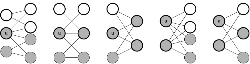
dis-tinct, not all three of these copies can be identical. As a re-sult, umust be contained in two different copies ofK2,2,
which means that at least one of the graphs shown in Fig-ure 1 must appear as a subgraph of G>τ0. Notice that by
the union bound, for any graphH = (VH, EH), the
prob-ability that it appears as a subgraph of G>τ0 is at most
(n+m)|VH|(p
>τ0)|EH| ≤ (3n)|VH|
Clogm
n
|EH|
.
How-ever, all graphs H in Figure 1 satisfy |EH| ≥ |VH|+ 1.
Hence, the probability that each of them appears as a sub-graph is at most(Clognn)O(1) =o(1). Using the union bound, the probability that at least one of these graphs appears as a subgraph ofG>τ0 is alsoo(1). This implies that the
proba-bility that at least one of the vertices is adjacent to more than two edges inE≥τ\E≥∗τ iso(1), as desired.
Finally, we note that Propositions 3.8 and 3.9 together im-ply Lemma 3.6.
3.5
Local Resilience of Perfect
r
-Matching
In this subsection, we show that in a random bipartite graph sampled from the Erd˝os-R´enyi random bipartite graph dis-tributionG(n, rn, p)with sufficiently largep, not only does a perfectr-matching exist, but the existence is also robust in the following sense: even if we remove edges from the graph, as long as not too many edges adjacent to each vertex are removed, a perfectr-matching still exists. Such “robust-ness” is known in the literature aslocal resilience. In par-ticular, the local resilience of perfect matchings was shown by Sudakov and Vu (2008). We will extend their proof to the case of perfectr-matchings. However, we note that our bound will be slightly weaker than theirs, since our main goal is to derive a bound that is sufficient for the algorithm to work and not to find the best possible parameters.
A typical method for establishing the existence of a per-fect matching, which was used both by Sudakov and Vu (2008) and by Erd˝os and R´enyi (1964), is to show that the graph satisfies the condition of Hall’s Marriage Theorem. For any graphGand any setS of vertices inG, denote by
NG(S)the set of vertices adjacent to at least one vertex inS.
Proposition 3.10 (Hall’s Marriage Theorem). Let G = (A, B, E) be any bipartite graph such that|A| = |B|. If
|NG(S)| ≥ |S|for all subsetsS ⊆A, thenGhas a perfect matching.
Recall thatG= (A, B, E)has a perfectr-matching if and only if the graph(A×[r], B, E0), where((a, `), b)∈E0iff
(a, b)∈E, has a perfect matching. Hence, Hall’s Marriage Theorem immediately extends tor-matchings:
Proposition 3.11. Let G = (A, B, E) be any bipartite graph such that|B|=r|A|. If|NG(S)| ≥r|S|for all sub-setsS ⊆A, thenGhas a perfectr-matching.
One way to show that the condition of Hall’s Marriage Theorem is satisfied is to show that there is at least one edge between any setsS⊆AandT ⊆Bof appropriate sizes. To ensure that the existence of a perfectr-matching is locally resilient, we need to show not only that one edge exists, but also that many edges exist. This can be done via standard concentration bounds. For any graphGand any setsS, T of vertices inG, denote byEG(S, T)the set of edges
connect-ing a vertex inSto a vertex inT.
Lemma 3.12. Let G = (A, B, E) be a graph sampled from the Erd˝os-R´enyi random bipartite graph distribution G(n, m, p)withp ≥ 64 logn m. Then, with high probability, the following holds for all subsetsS ⊆AandT ⊆Bsuch that|T|=m−r|S|+ 1:
|EG(S, T)|>(16 logm)·min{|S|,|T|}. (1)
The proof of Lemma 3.12 can be found in the full version of this paper (Manurangsi and Suksompong, 2018).
With Lemma 3.12 ready, we now establish the local re-silience of the existence of perfect r-matchings in random graphs.
Lemma 3.13. Let G = (A, B, E) be a graph sampled from the Erd˝os-R´enyi random bipartite graph distribution G(n, m, p)withp ≥ 64 logn m. Then, with high probability, for any subgraphH = (A, B, E0)ofGwith maximum de-gree at most16 logm, the graphG−H = (A, B, E\E0)
contains a perfectr-matching.
Proof. From Lemma 3.12, with high probability, (1) holds for all S ⊆ A, T ⊆ B with|T| = m−r|S|+ 1. We claim that this implies thatG−H = (A, B, E\E0) con-tains a perfectr-matching. Suppose for the sake of contra-diction that G−H does not contain an r-perfect match-ing. Proposition 3.11 implies that there exists a setS ⊆ A
such that|NG−H(S)| ≤ r|S| −1. LetT be any subset of B\NG−H(S)of sizem−r|S|+1. SinceT∩NG−H(S) =∅,
we haveEG−H(S, T) =∅. However, by (1),|EG(S, T)|>
(16 logm)·min{|S|,|T|}. This means that at least one ver-tex inS∪T has degree more than16 logminH, which is a contradiction.
3.6
Putting Things Together
With Lemmas 3.6 and 3.13 in hand, we can (finally) prove Lemma 3.5.
u u u
u u
Figure 1: All possible unions of two distinct complete bipartite graphsK2,2which share at least one vertexu, up to isomorphism.
The shaded vertices constitute one copy ofK2,2whereas the thickened vertices constitute another.
defined as in Algorithm 1. Recall also thatG≥τis distributed
according to the Erd˝os-R´enyi random bipartite graph dis-tributionG(n, m, p)withp = Pru∼U[u ≥ τ] ≥ 64 logn m. It therefore follows from Lemma 3.13 that a perfect r -matching exists inG∗≥τ with high probability.
4
Non-Existence
Our main non-existence result states that envy-free alloca-tions are unlikely to exist ifm = O(nlogn/log logn)is not “close to” being a multiple ofn. This improves upon them =n+o(n)lower bound of Dickerson et al. (2014) and comes to within aΘ(log logn)factor of matching their upper bound.
Theorem 4.1. For any real numbersθ >0,∈(0,1), and q≥1, there existsc >0depending only onθ, , qsuch that the following holds: For any positive integerr≤ log logclognn, if m∈[rn+n,(r+ 1)n−n]andU is(θ, q)-polynomially bounded below at 1, then, with high probability, there is no envy-free allocation.
We remark that since we only require the distribution to be polynomially bounded below, the assumptionq≥1does not introduce a loss of generality. Next, we give an overview of the proof of Theorem 4.1; the full proof can be found in the full version of this paper (Manurangsi and Suksompong, 2018).
The proof is based on the first moment method; the key is to show that for any fixed allocation, the probability (over the random utilities drawn) that it is envy-free is 1/nm. Since there arenmpossible allocations, the union bound
im-plies that with high probability, no envy-free allocation ex-ists.
To give an intuition for this bound, let us consider a sim-plified setting wherem = (r+ 0.5)nand the distribution
U is uniform on[0,1]. Intuitively, the “more balanced” the allocation is, the harder it is to bound the probability that the allocation is envy-free. Following this intuition, let us consider the “most balanced” allocation where0.5nagents receiver+ 1items and the remaining agents receiveritems. The key observation is that, for the allocation to be envy-free for every agent in the latter group, any such agent must have utility at mostrfor ther+ 1items in the bundle of any agent in the first group. For a fixed agent in the second group and a fixed agent in the first group, this happens with probability
at most1−1/(r+ 1)r+1. Indeed, if each of ther+ 1items
yields utility at leastr/(r+ 1)to the agent, the requirement is not satisfied. Now, since there are 0.25n2 such pairs of
agents, the probability that this fixed allocation is envy-free
is at most 1− 1 (r+1)r+1
0.25n2
= expΘ(r+1)−n2r+1
.
Hence, as long asrlogn/log logn, this term is at most, say,exp(−n1.9), which is indeed much smaller thann−m.
The full proof proceeds along the lines of the argument above, but we need to be more careful as we must also deal with other “less balanced” allocations.
5
Discussion
In this paper, we study the existence and non-existence of envy-free allocations and essentially close the gap left open by Dickerson et al. (2014) with regard to the transition be-tween the two phases. On the positive side, we show that if the number of items is a multiple of the number of agents, an envy-free allocation is likely to exist as long as the for-mer quantity is at least twice the latter. On the negative side, we show that if the number of items is not “close to” being a multiple of the number of agents, an envy-free allocation is unlikely to exist even when the former quantity exceeds the latter by almost a logarithmic factor. Both of our results make use of several new ideas that may be useful for other problems in fair division.
As we mentioned earlier, all of the works on the asymp-totic existence of fair allocations thus far have assumed that agents are endowed with additive utilities. While additivity provides a reasonable trade-off between simplicity and ex-pressiveness, it would be interesting to establish analogous results that hold for more general classes of utilities. Going beyond additivity introduces several complications; for ex-ample, the welfare-maximizing allocation is no longer sim-ply the one that assigns every item to the agent who values it most, and giving an agent several goods that she values highly does not guarantee that the agent will also have a cor-respondingly high value for the whole bundle. Nevertheless, a starting point may be to prove results for specific distribu-tions over utilities from a well-structured class such as that of submodular valuations.
(Segal-Halevi and Nitzan, 2016; Segal-(Segal-Halevi and Suksompong, 2018; Suksompong, 2018a,b). The agents in each group share the same set of items but may have different prefer-ences. This is the case, for example, when dividing house-hold goods among families or resources between depart-ments in a university. Manurangsi and Suksompong (2017) generalized the results of Dickerson et al. (2014) to the group setting and left a logarithmic gap between existence and non-existence. We are hopeful that the techniques we introduce in the present work will help towards closing this gap as well.
Acknowledgments
This work was partially supported by NSF Awards CCF-1655215, CCF-1813188, CCF-1815434, and by a Stanford Graduate Fellowship. We would like to thank the anony-mous reviewers for their helpful comments.
References
Amanatidis, G.; Markakis, E.; Nikzad, A.; and Saberi, A. 2017. Approximation algorithms for computing max-imin share allocations. ACM Transactions on Algorithms
13(4):52.
Amanatidis, G.; Birmpas, G.; and Markakis, E. 2018. Com-paring approximate relaxations of envy-freeness. In Pro-ceedings of the 27th International Joint Conference on Arti-ficial Intelligence, 42–48.
Barman, S.; Krisnamurthy, S. K.; and Vaish, R. 2018. Find-ing fair and efficient allocations. InProceedings of the 19th ACM Conference on Economics and Computation, 557–574. Biswas, A., and Barman, S. 2018. Fair division under cardi-nality constraints. InProceedings of the 27th International Joint Conference on Artificial Intelligence, 91–97.
Brams, S. J., and Taylor, A. D. 1996. Fair Division: From Cake-Cutting to Dispute Resolution. Cambridge University Press.
Caragiannis, I.; Kurokawa, D.; Moulin, H.; Procaccia, A. D.; Shah, N.; and Wang, J. 2016. The unreasonable fairness of maximum Nash welfare. InProceedings of the 17th ACM Conference on Economics and Computation, 305–322.
Conitzer, V.; Freeman, R.; and Shah, N. 2017. Fair public decision making. InProceedings of the 18th ACM Confer-ence on Economics and Computation, 629–646.
Dickerson, J. P.; Goldman, J.; Karp, J.; Procaccia, A. D.; and Sandholm, T. 2014. The computational rise and fall of fairness. In Proceedings of the 28th AAAI Conference on Artificial Intelligence, 1405–1411.
Erd˝os, P., and R´enyi, A. 1961. On a classical problem of probability theory. Magyar Tudom´anyos Akad´emia Matem-atikai Kutat´o Int´ezet´enek K¨ozlem´enyei6:215–220.
Erd˝os, P., and R´enyi, A. 1964. On random matrices. Pub-lications of the Mathematical Institute of the Hungarian Academy of Sciences8:455–461.
Foley, D. K. 1967. Resource allocation and the public sector.
Yale Economics Essays7(1):45–98.
Kurokawa, D.; Procaccia, A. D.; and Wang, J. 2016. When can the maximin share guarantee be guaranteed? In Pro-ceedings of the 30th AAAI Conference on Artificial Intelli-gence, 523–529.
Lipton, R. J.; Markakis, E.; Mossel, E.; and Saberi, A. 2004. On approximately fair allocations of indivisible goods. In
Proceedings of the 5th ACM Conference on Electronic Com-merce, 125–131.
Manurangsi, P., and Suksompong, W. 2017. Asymptotic existence of fair divisions for groups. Mathematical Social Sciences89:100–108.
Manurangsi, P., and Suksompong, W. 2018. When do envy-free allocations exist? CoRRabs/1811.01630.
Moulin, H. 2003.Fair Division and Collective Welfare. MIT Press.
Plaut, B., and Roughgarden, T. 2018. Almost envy-freeness with general valuations. In Proceedings of the 29th An-nual ACM-SIAM Symposium on Discrete Algorithms, 2584– 2603.
Segal-Halevi, E., and Nitzan, S. 2016. Envy-free cake-cutting among families. CoRRabs/1607.01517.
Segal-Halevi, E., and Suksompong, W. 2018. Demo-cratic fair allocation of indivisible goods. In Proceedings of the 27th International Joint Conference on Artificial In-telligence, 482–488.
Stromquist, W. 1980. How to cut a cake fairly.The American Mathematical Monthly87(8):640–644.
Sudakov, B., and Vu, V. H. 2008. Local resilience of graphs.
Random Structures and Algorithms33(4):409–433. Suksompong, W. 2016. Asymptotic existence of proportion-ally fair allocations. Mathematical Social Sciences81:62– 65.